in the population sciences published by the Max Planck Institute for Demographic Research Doberaner Strasse 114 · D-18057 Rostock · GERMANY www.demographic-research.org
DEMOGRAPHIC RESEARCH
VOLUME 5, ARTICLE 4, PAGES 79-124
PUBLISHED 13 NOVEMBER 2001
www.demographic-research.org/Volumes/Vol5/4/
DOI: 10.4054/DemRes.2001.5.4
Attrition in Longitudinal Household
Survey Data
Harold Alderman
Jere R. Behrman
Hans-Peter Kohler
John A. Maluccio
Susan Cotts Watkins
1 Introduction 80
2 Some Theoretical Aspects of the Effects of Attrition on Estimates
82
2.1 Attrition bias due to selection on observables and unobservables
83
2.2 Testing for attrition bias 87
3 Data and Extent of Attrition 88
3.1 Bolivian Pre-School Program Evaluation Household Survey Data. El Proyecto Integral de Desarrollo Infantil (PIDI)
89
3.2 The Kenyan Ideational Change Survey (KDICP) 89 3.3 KwaZulu-Natal Income Dynamics Study (KIDS) 90
4 Some Attrition Tests for the Bolivian, Kenyan, and South African Samples
92
4.1 Comparison of Means for Major Outcome and Control Variables
93
4.2 Probits for Probability of Attrition 99 4.3 Do Those Lost to Follow-up have Different
Coefficient Estimates than Those Re-interviewed?
103
5 Conclusions 113
6 Acknowledgements 114
Notes 116
Attrition in Longitudinal Household Survey Data:
Some Tests for Three Developing-Country Samples
Harold Alderman 1, Jere R. Behrman 2, Hans-Peter Kohler 3, John A. Maluccio 4,
and Susan Cotts Watkins 5
Abstract
Longitudinal household data can have considerable advantages over much more widely used cross-sectional data for capturing dynamic demographic relationships. However, a disturbing feature of such data is that there is often substantial attrition and this may make the interpretation of estimates problematic. Such attrition may be particularly severe where there is considerable migration between rural and urban areas. Many analysts share the intuition that attrition is likely to be selective on characteristics such as schooling and thus that high attrition is likely to bias estimates. This paper considers the extent and implications of attrition for three longitudinal household surveys from Bolivia, Kenya, and South Africa that report very high per-year attrition rates between survey rounds. Our estimates indicate that: (a) the means for a number of critical outcome and family background variables differ significantly between those who are lost to follow-up and those who are re-interviewed; (b) a number of family background variables are significant predictors of attrition; but (c) nevertheless, the coefficient estimates for standard family background variables in regressions and probit equations for a majority of the outcome variables considered in all three data sets are not affected significantly by attrition. Therefore, attrition apparently is not a general problem for obtaining consistent estimates
1 Development Research Group, World Bank, 1818 H Street NW, Washington D.C. 20433, USA. Email: [email protected].
2 Population Studies Center, McNeil 160, 3718 Locust Walk, University of Pennsylvania, Philadelphia, PA 19104-6297, USA. Email: [email protected].
3 Max-Planck Institute for Demographic Research, Doberaner Str. 114, 18057 Rostock, Germany. Email: [email protected].
4 International Food Policy Research Institute, 2033 K Street NW, Washington D.C. 20006, USA. Email: [email protected].
of the coefficients of interest for most of these outcomes. These results, which are very similar to those for developed countries, suggest that multivariate estimates of behavioral relations may not be biased due to attrition and thus support the collection of longitudinal data.
1. Introduction
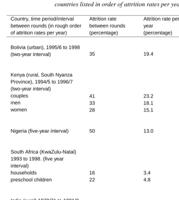
Longitudinal (or panel) household data can have considerable advantages over more widely available cross-sectional data for social science analysis. Longitudinal data permit (1) tracing the dynamics of behaviors, (2) identifying the influence of past behaviors on current behaviors, and (3) controlling for unobserved fixed characteristics in the investigation of the effect of time-varying exogenous variables on endogenous behaviors. These advantages are substantial for demographers studying processes that occur over time including the impact of programs on subsequent behavior that often use time-varying exogenous variables. As a result, the advantages are also increasingly appreciated: for example, a review of articles published in the journal Demography indicates that only 26 articles using longitudinal data appeared between 1980-1989, while there were 65 between 1990-2000. Unfortunately, the collection of longitudinal data is likely to be difficult and expensive, and some researchers, such as Ashenfelter, Deaton, and Solon (1986), have questioned whether the gains are worth the costs. One problem in particular that has concerned analysts is that sample attrition may lead to selective samples and make the interpretation of estimates problematic. Many analysts share the intuition that attrition is likely to be selective on characteristics such as schooling and thus that high attrition is likely to bias estimates made from longitudinal data. While there has been some work on the effect of attrition on estimates using developed-country samples, little has been done using data from developing countries, where considerable migration between rural and urban areas typically exacerbates the problem of attrition. Table 1 summarizes the attrition rates in a number of longitudinal data sets from developing countries. While these vary widely (ranging from 6 to 50 percent between two survey rounds and 1.5 to 23.2 percent per year between survey rounds), often there is considerable attrition.
Table 1: Attrition rates for longitudinal household survey data in developing countries listed in order of attrition rates per year
Country, time period/interval between rounds (in rough order of attrition rates per year)
Attrition rate between rounds (percentage)
Attrition rate per year
(percentage) Source
Bolivia (urban), 1995/6 to 1998
(two-year interval) 35 19.4
Present study (also see Alderman and Behrman 1999)
Kenya (rural, South Nyanza Province), 1994/5 to 1996/7 (two-year interval) couples
men women
41 33 28
23.2 18.1 15.1
Present study (also see Behrman, Kohler, and Watkins 2001)
Nigeria (five-year interval) 50 13.0 Renne (1997)
South Africa (KwaZulu-Natal) 1993 to 1998. (five year interval)
households preschool children
16 22
3.4 4.8
Present study (also see Maluccio 2001)
India (rural) 1970/71 to 1981/2
(11-year interval) 33 3.6
Foster and Rosenzweig 1995
Malaysia (12-year interval) 25 2.4 Smith and Thomas 1997
Indonesia 1993 to 1997
(four-year interval) 6 1.5
Thomas, Frankenberg, and Smith 1999
Note: The annual attrition rate is calculated as 1- (1-q)1/T
Province) rural and urban household survey designed for more general purposes, with survey rounds in 1993 and 1998. The different aims of the projects and the variety of outcome measures facilitate generalization, at least for survey areas such as these that are relatively poor and experiencing considerable mobility.
Drawing on recent studies on attrition in longitudinal surveys for developed countries, the next section summarizes theoretical aspects of the effects of attrition on estimates. Section 3 describes the three datasets used in this study and section 4 presents some tests for the implications of attrition between the first and the second rounds of the three surveys. Section 5 summarizes our conclusions.
2. Some Theoretical Aspects of the Effects of Attrition on Estimates
Most of the previous work on attrition in large longitudinal samples is for developed economies, for example, the studies published in a special issue of The Journal of Human
Resources (Spring 1998) on Attrition in Longitudinal Surveys (for related statistical
literature on missing values and survey non-response see for instance Little and Rubin 1987 or Ahlo 1990). The striking result of the studies presented in the Journal of Human
Resources (JHR) is that the biases in estimated socioeconomic relations due to attrition are
small despite attrition rates as high as 50 percent and significant differences between those re-interviewed and those lost to follow-up for many important characteristics. For example, Fitzgerald, Gottschalk and Moffitt (1998) summarize:
By 1989 the Michigan Panel Study on Income Dynamics (PSID) had experienced approximately 50 percent sample loss from cumulative attrition from its initial 1968 membership… (p. 251)
We find that while the PSID has been highly selective on many important variables of interest, including those ordinarily regarded as outcome variables, attrition bias nevertheless remains quite small in magnitude. … (most attrition is random)... (p. 252)
Although a sample loss as high as [experienced] must necessarily reduce precision of estimation, there is no necessary relationship between the size of the sample loss from attrition and the existence or magnitude of attrition bias. Even a large amount of attrition causes no bias if it is ‘random’ … (p. 256)
Income and Program Participation (SIPP), the National Longitudinal Surveys of Labor Market Experience (NLS), and the Labor Supply Panel Survey in the Netherlands (Falaris and Peters 1998; Lillard and Panis1998; Van den Berg and Lindeboom 1998; Zabel 1998; Ziliak and Kniesner 1998).
This absence of relevant distortions in parameter estimates due to attrition can be understood once the relation between the mechanisms leading to attrition and the empirical model of interest is made explicit.
2.1 Attrition bias due to selection on observables and unobservables
Fitzgerald, Gottschalk, and Moffitt (1998) provide an econometric framework for the analysis of attrition in which the common distinction between selection on variables observed in the data and variables that are unobserved is used to develop tests for attrition bias and correction factors to eliminate it. (Note 1) This framework assumes a panel study that attempts to interview the same sample of respondents (or households, etc.) for say, T annual survey rounds at times t = 1, … T. The initial sample at time t=1 is assumed to be a random or stratified random sample of the population. Attrition of a respondent at time
t, denoted At, is then defined as the fact that the respondent participates in all survey waves
1, …, t-1, but does not participate in any survey wave from time t onwards (Note 2). Common causes for attrition are death or migration of the respondent, or refusal to participate due to saturation or frustration with a particular survey. The respondent thus reports information for the dependent and explanatory variables for the survey waves 1, …,
t-1. Neither the dependent variable nor time-varying explanatory variables are observed
from survey wave t onwards. (Note 3) Analyses of and adjustments for attrition at time t can therefore be based on fixed characteristics of the respondent, lagged time-varying variables pertaining to periods prior to time t, and information that do not require the completion of an interview, such as interviewer characteristics and location of residence. The central concern in the analyses of attrition – and of missing data in general – is selection bias, that is, a distortion of the estimation results due to non-random patterns of attrition. The common distinction is between attrition that is completely random, attrition that is selective on variables unobserved in the data, and attrition that is selective on variables observed in the data. The latter can be further distinguished between attrition that leads to ignorable selection on observables (the statistical literature on missing data also uses the terms “missing-at-random”) or non-ignorable selection on observables.
attrition, one determines whether or not there is selection on observables. Second, if there is selection on observables, one determines whether this attrition is ignorable – and thus does not bias the estimates of interest – or whether it is non-ignorable. In the latter case, the analyses need to adjust for attrition since otherwise selection leads to biased inferences about relevant parameters. The available methods to correct for attrition on observables are often relatively easy to implement and rely on relatively weak assumptions, in contrast to the methods that are required in order to adjust for selection on unobservables. While selective attrition on unobservables potentially remains a problem even after the analyses account for selection on observables, using as much information as possible about selection on observables in the panel helps to reduce the amount of residual, unexplained variation in the data due to attrition. Controlling for selection on observables thus will likely reduce the biases due to the selection on unobservables. (Note 4)
More formally, consider the survey wave at time t and assume that what is of interest is a conditional population density f(yt|xt) where yt is a scalar dependent variable and xt is
an observed scalar independent variable (for illustration; in practice the extension treating
xt as a vector, which potentially includes lagged dependent variables, fixed characteristics
of the respondent, and lagged time-varying characteristics of the respondent, is straightforward; see for instance Fitzgerald et al. 1998). In particular, we assume the linear parametric model
yt = 0 + 1xt + t,
yt observed if At = 0 (1)
where t is a mean-zero random variable, and At is an attrition indicator equal to 1 if an
observation is missing its value of yt because of attrition, and equal to zero if an observation
is not missing its value of yt. For identification, we assume in this theoretical model that the
variable xt is observed for both attritors and non-attritors, as would be the case if it were a
time-invariant or lagged variable, for example. The presence of attrition implies that Eq. (1) can only be estimated for respondents that are interviewed at time t, that is for observations for which At=0 and yt is observed.
The analysis of these observed data can therefore determine the density f(yt|xt, At=0)
that is conditional on xt and At=0. Additional information or restrictions are necessary in
order to infer the density of primary interest, f(yt|xt), from the observed data. That is, we
seek f(yt) conditional on xt but not on At=0.
This additional information can come from the probability of attrition, Pr(At=0|yt, xt, zt), where zt is an auxiliary variable (or vector) that is assumed to be observable for all units
but is not included in xt. In particular, in the straightforward generalization to vectors, zt can
respondent, lagged time-varying characteristics, and variables that do not require the completion of an interview, such as interviewer characteristics and location of residence. (The set of respondent characteristics that can potentially be included in zt is restricted to
those characteristics that are not already included among the variables in xt.)
Linearizing the probability of attrition implies a process of the form
At* = 0 + 1xt + 2zt + t (2)
At = 1 if At*$ 0
= 0 if At* < 0, (3)
where At* is a latent index and attrition occurs if this index is equal or larger to zero and t
is a mean-zero random influence on the attrition probability.
Attrition can then be classified as follows (this classification differs slightly from that proposed by Fitzgerald et al. 1998 and has a more direct relation to the statistical literature on missing data; see also Kohler 2001):
Attrition exhibits selection on unobservables if Pr(At=0|yt, xt, zt) 3UAt=0|xt, zt), so
that the attrition function cannot be reduced from Pr(At=0|yt, xt, zt). In the specific
parametric model in Eqs. (1 – 3), therefore, selection on unobservables occurs if vt is not
independent of t|xt, where t|xt is a shorthand notation for the error term t conditional on xt.
Attrition exhibits selection on observables if
Pr(At=0|yt, xt, zt) = Pr(At=0|xt, zt), (4)
that is, if, conditional on xt and zt, the attrition probability is independent of the dependent
variable yt and therefore of the unobserved factors entering the error term t in relation (1).
On one hand, this selection on observables is ignorable if (a) yt and zt are independent
conditional on xt and At=0, or (b) the attrition function in Eq. (4) can be further reduced to
Pr(At=0|xt, zt) = Pr(At=0|xt), i.e., the probability of attrition is independent of the variable zt. Ignorable selection on observables implies that the linear regression of relation (1) on
the basis of the observed data on non-attritors leads to unbiased estimates of the coefficients
β0 and β1. In this case, no specific methods are required to control or adjust for attrition.
On the other hand, selection on observables is non-ignorable when neither condition (a) nor (b) holds. In this case, standard linear regression analysis of relation (1) does not yield unbiased estimates of the coefficients β0 and β1, and alternative estimation techniques
Selection on observables in this parametric model is non-ignorable when neither condition (a’) nor (b’) holds.
Attrition is completely at random if the attrition function Pr(At=0|yt, xt, zt) can be
reduced to Pr(At=0) and attrition neither depends on the dependent variable yt nor the
observed variables xt and zt. In our specific model, attrition is completely at random if vt is
independent of t|xt and 1 and 2 in Eq. (2) are zero.
Ordering these attrition patterns in terms of their assumptions from more restrictive to less restrictive yields: completely random attrition < selective attrition on observables < selective attrition on unobservables. Completely random attrition is unlikely in most panel studies, and if it exists, it does not result in biases of parameter estimates. Attrition that is selective on observables and unobservables, on the other hand, is probably a common phenomenon in most panel studies, and we will briefly discuss the statistical approaches to overcome the biases that are potentially caused by such attrition.
Selection on unobservables is often presented as dependent on the estimation of the attrition index equation (2) (see for instance Maddala 1983 or Powell 1994 for discussions of this approach). Identification, however, usually relies on nonlinearities in the index equation or an exclusion restriction, i.e., the existence of a variable zt – often loosely termed
“instrument” – that predicts attrition but is independent of t|xt and not included in xt. It is
difficult to rationalize most such exclusion restrictions because, for example, personal characteristics that affect attrition might also directly affect the outcome variable, i.e., they should be in xt or are correlated with t|xt. There may be some such identifying variables in
the form of variables that are external to individuals and not under their control, such as characteristics of the interviewer in the various rounds (Zabel 1998, Maluccio 2001). However, in the PSID and potentially also in other panel studies the interviewers are assigned on the basis of respondent characteristics, in which case this strategy is also not feasible. In general, therefore, selection on unobservables presents an obstacle to accurate parameter estimation. Most promising, in our opinion, is therefore to test and – if necessary adjust – for non-ignorable selection on observables by using as much information as possible about selection in the panel. This reduces the amount of residual, unexplained variation due to attrition left over in the data and it lessens the scope for selection on unobservables for which few feasible statistical solutions exist.
If there is non-ignorable selection on observables, the critical variable is zt, a variable
that affects attrition propensities and that is also related to the density of yt conditional on xt due to the fact that zt is not independent of t|xt. In this sense, zt is “endogenous to yt.”
Indeed, a lagged value of yt can play the role of zt if it is not in the structural relation being
estimated but is related to attrition.
Fitzgerald et al. (1998) show formally that, under the selection on observables restriction in Eq. (4), the complete population density f(yt|xt) can be computed from the
f(yt|xt) = Jyt, zt | xt, At=0) w(zt, xt) dzt, (5)
where
w(zt, xt) = Pr(At=0|xt) / Pr(At=0|zt, xt) (6)
are normalized weights (the proof of Eq. 5 is also given in the appendix of this paper). (Note 5) The numerator of Eq. (6) is the probability of remaining in the sample (i.e., non-attrition) conditional on xt, and the denominator is the probability of remaining in the
sample conditional on zt and xt. The weights w(zt, xt) in Eq. (6) can be estimated from the
data when both xt and zt are observed. This is the case when – as we have assumed above
– xt and zt contain either time-invariant or lagged time-varying characteristics of the
respondent or variables that do not require a completed interview. (Note 6)
The intuition for Eqs. (5 – 6) is in the spirit of weighting (panel) observations with the inverse of the probability that an observation is included (as in stratified samples, for instance); in the above case pertaining to attrition, this probability is replaced by the function of attrition probabilities in Eq. (6). Because both the weights and the conditional density g are identifiable and estimable from the data, the complete-population density
f(yt|xt) is estimable as well as its moments such as the expected value Eyt = 0 + 1xt implied
by Eq. (1). This result is particularly important since it implies that in the linear model in Eq. (1) the parameters 0 and 1 can be estimated without bias, despite the presence of
selective attrition on observables, via a weighted least squares regression (WLS) that uses the weights defined in Eq. (6).
Inspection of Eqs. (5) and (6) also reveals the cases when selection on observables can be ignored. In particular, if zt is not a determinant of attrition, the weights in Eq. (6) equal
one and no attrition bias is present. If yt and zt are independent conditional on xt and At=0,
the density g in Eq. (5) factors and it can again be shown that the unconditional density
f(yt|xt) equals the conditional density and there is no attrition bias.
2.2 Testing for attrition bias (Note 7)
the United States). Unfortunately, only very limited possibilities for such comparisons exist for most panels, and such comparisons are especially difficult in developing countries. Due to this limited ability to detect selective attrition on unobservables with the datasets examined in this paper, we do not discuss this approach further nor do we perform the corresponding tests.
Testing for selection bias due to selective attrition on observables, on the other hand, is possible in most panel studies and we will focus on these approaches. The two sufficient conditions that render the selection on observables through attrition ignorable are either (1)
zt does not affect At or (2) zt is independent of yt conditional on xt and At=0. Specification
tests can be based on either of these two conditions. One test is simply to determine whether candidate variables for zt (for example, lagged values of y) significantly affect At.
Another test is based on Becketti, Gould, Lillard, and Welch (1988). In the BGLW test, the value of y at the initial wave of the survey (y1) is regressed on respondent’s characteristics
at the initial wave (x1) and on A, which denotes the event that a respondent becomes an
attritor at some time during the survey (i.e., At equals one for some t in 2,…,T). The test for
attrition is based on the significance of A in that equation. This test is closely related to the test based on regressing A on x1 and y1, which is a direct estimation of the attrition
probability in Eqs. (2 – 3) in the special case when the y1 is used to represent the auxiliary
variable zt. In fact, the direct estimation of the attrition probability and the BGLW test are
simply inverses of one another (Fitzgerald et al. 1998). (Note 8)
Clearly, if there is no evidence of attrition bias from these specification tests, this suggests that the attrition on observables is ignorable. (Since the null-hypothesis of our attrition tests is the absence of attrition, the fact that there is not significant evidence of attrition bias from these specification tests is no proof that such bias does not exist. It does, however, show that the possible bias is too small to be detectable given the power of the available tests. This limitation is a general problem of statistical inference and not restricted to the specification tests for attrition).
If the specification tests suggest that attrition on observables is ignorable, then the desired information on f(yt|xt) can be directly inferred from the conditional density f(yt|xt, At=0) (under the assumption that there is no selective attrition on unobservables). If the
above tests detect non-ignorable selection on observables due to attrition, the resulting biases in the inference of 0 and 1 in Eq. (1) can be avoided by using a weighted least
squares methodology with the weights given in Eq. (6).
3. Data and Extent of Attrition
3.1 Bolivian Pre-School Program Evaluation Household Survey Data. El Proyecto Integral de Desarrollo Infantil (PIDI)
PIDI is a targeted urban early child development project expected to improve the nutritional status and cognitive development of children who participate and to facilitate the labor force participation of their caregivers. PIDI delivers child services through childcare centers located in the homes of local women who have been trained in childcare. The program provides food accounting for 70 percent of the children’s nutritional needs, health and nutrition monitoring, and programs to stimulate the children’s social and intellectual development. The PIDI program was designed to facilitate ongoing impact evaluation through the collection of longitudinal data.
Eligibility for PIDI at the time of the collection of the first and second rounds of data was based on an assessment of social risk. As a result of this selection, children who attend a PIDI center are, on average, from poorer family backgrounds than children who live in the same communities but who do not attend a PIDI center (Behrman, Cheng and Todd 2001). The first PIDI evaluation data set (Bolivia 1) was collected between November 1995 and May 1996 and consisted of 2,047 households. (Note 9) The follow-up survey (Bolivia 2) was collected in the first half of 1998 and consisted of interviews in the 65 percent of the original 2,047 households that could be located (plus an additional 3,453 households that were not visited in Bolivia 1). The attrition rate of 35 percent for Bolivia 1 is relatively high, which raised concern about whether reliable inferences could be drawn from analysis of Bolivia 2.
3.2 The Kenyan Ideational Change Survey (KDICP)
at www.pop.upenn.edu/networks). The attrition rates between the two surveys were 33 percent for men, 28 percent for women, and 41 percent for couples (Table 1). (Note 10) These rates are comparable to the 35 percent reported for the Bolivian data.
Table 2 summarizes data on the reported causes of attrition for men and women as obtained from other household members for most individuals who were interviewed in Kenya 1 but not in Kenya 2. (Note 11) Nyanza Province has a relatively high level of AIDS: mortality between the surveys accounted for 18 percent of the reasons given for men’s attrition, but only half as much (10 percent) for women. For both men and women the leading explanation was migration, accounting for 59 percent of the reasons given for women and 48 percent of the reasons given for men. Because this is a patrilocal society, a significant share of this migration (over one-third) for women was associated with divorce or separation, but this was not a major factor for men. Not being found at home after at least three visits by interviewers was the next most common explanation for attrition in Kenya 2, accounting for about one-sixth of the reasons given for both men (18 percent) and women (16 percent). Explicitly refusing or claiming to be too busy or sick to participate accounted for slightly smaller percentages – 16 percent for men and 11 percent for women (with most of this gender difference accounted by “other,” which is 4 percent for women but 0 percent for men).
3.3 KwaZulu-Natal Income Dynamics Study (KIDS)
Table 2: Reported reasons for men’s and women’s attrition in Kenyan (KDICP) survey
Men Women
Reason for attrition: Number Percentage Number Percentage
Working, moved to, or visiting outside Nyanza Province
Working, moved to, or visiting elsewhere in Nyanza Province
Not home
Refused
Sick or busy
Deceased
Separated, divorced, then moved away
Other
45
51
36
26
6
37
n/a
0
22.4
25.4
17.9
12.9
3.0
18.4
n/a
0.0
21
56
32
20
3
20
42
11
10.3
27.6
15.8
9.9
1.5
9.9
20.7
4.4
Total 201 205
Note: n/a = not available
An important aspect of the South Africa resurvey – differentiating it further from the Bolivian and Kenyan longitudinal surveys – is that, when possible, the interviewer teams tracked, followed, and re-interviewed households that had moved. (Note 13) Hence, in the South Africa survey migration does not imply automatic attrition from the sample. In addition to reducing the level of attrition and allowing analysis of migration behavior, tracking and following plausibly reduced biases introduced by attrition, a claim we evaluate below.
In 1993, the KwaZulu-Natal sample contained 1,354 households (215 Indian and 1,139 African). Of the target sample, 1,152 households (84 percent) with at least one 1993 member were successfully re-interviewed in 1998 (Maluccio 2001). As in most surveys in developing countries, refusal rates were very low, less than 1 percent. The remaining households that could not be re-interviewed were either verified as having moved but could not be tracked (7 percent) or left no trace (8 percent). Had the sixty households that had moved but were successfully tracked not been followed, 79 percent of the target households would have been re-interviewed. Put another way, the tracking procedures yielded a 25 percent reduction in the number of households that were lost to follow-up.
Re-interview rates were slightly higher in urban than in rural areas. Offsetting that success was a follow-up rate of 78 percent (of 215 households) for Indian households, all of which were urban. The follow-up rate for rural Africans was 83 percent (of 825 households). There were no major differences in the analysis of attrition when we considered the rural and urban samples separately; therefore we present only the results where we pooled them.
The discussion of attrition between South Africa 1 and South Africa 2 to this point has focused on attrition at the household level. For an analysis of individual level outcomes, however, attrition at the individual level is the relevant measure. Because a household was considered to be found if at least one 1993 member was re-interviewed, individual-level attrition for the entire sample is necessarily higher than household attrition (although this need not be the case for subsamples of individuals). Focusing on the sample of children aged 6 – 72 months for whom there is complete information on height, weight, and age in 1993, for example, 78 percent of 897 children were re-interviewed as household members in 1998, indicating one-third more attrition than at the household level. (Note 14).
4. Some Attrition Tests for the Bolivian, Kenyan, and South African
Samples
children in the South African sample. However, studies for developed countries suggest that while attrition of this magnitude may be selective, it need not significantly affect estimated multivariate relations. To test this, we conducted three sets of tests of attrition as it relates to observed variables in the data, using some of the tests presented by Fitzgerald, Gottschalk, and Moffitt (1998). We begin with a comparison of means, since the intuition that attrition is likely to bias estimates is often made on the basis of such univariate comparisons. We then estimate probits for the probability of attrition in order to ask what variables predict attrition comparing univariate and multivariate estimates. Lastly, we test whether coefficient estimates for a set of relations of interest to the objectives of the studies differ for two subsamples, one that is lost to follow-up and one that is re-interviewed.
4.1 Comparison of Means for Major Outcome and Control Variables
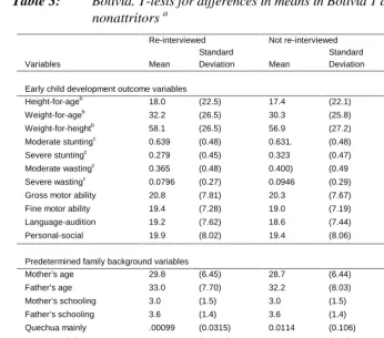
First, we compared means for major outcome and control variables measured in the first rounds of the respective data sets for those subsequently lost to follow-up versus those who were re-interviewed (Tables 3, 4, and 5). Major characteristics are defined with respect to the interests of the project for which these data were collected.
Bolivia: A number of means for those lost to follow-up differ statistically from those
who eventually were re-interviewed: rates of severe stunting, moderate wasting, the fraction reporting that they mainly spoke Quechua at home, weight-for-age, gross motor ability test scores, fine motor ability test scores, language-audition test scores, personal-social test scores, mother’s age, father’s age, home ownership, fraction with both parents present, number of rooms in the home, number of siblings, ownership of durables, mother having job, and household income (Table 3). All of these observable characteristics distinguish the two subsamples at least at the 10 percent significance level, and show that in the first round of the data (Bolivia 1) children who were worse off in terms of these measures were more likely to be lost to follow-up before the second round than those who would eventually be re-interviewed. Among the fourteen predetermined parental and household level variables in Table 3, eleven differ significantly for the two groups at least at the 10 percent significance level. Thus, both in terms of child development outcome variables and family background variables, attrition seems to be systematically more likely for children who are worse off. Such systematic differences, together with the high attrition rates, may cause concern about what can be inferred with confidence from these longitudinal data.
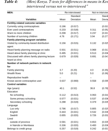
Kenya: For the Kenyan data, both males and females lost to follow-up have higher
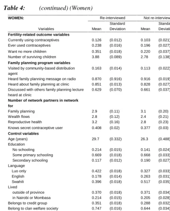
women (ever-use of contraceptives, residence in the sublocation of Owich) or for women but not for men (want no more children, visited by community-based distribution agent, speaks Luo only, belongs to credit group or to clan welfare society, residence in the sublocation of Wakula South). On the other hand, the means do not differ for the subsamples of either men or women for a number of characteristics (currently using contraceptives, heard about family planning at clinic, discussed family planning with others, number of partners in networks, primary schooling, lived outside of province, polygamous household).
Therefore, it appears that attrition is selective in terms of some ‘modern’ characteristics (including some of the outcome variables that these data were designed to analyze) with selectivity more strongly related to women’s characteristics. But the means for many characteristics, including those for most of the indicators of social interaction, the impact of which is central to the project for which these data were gathered, do not differ significantly between those lost to follow-up and those re-interviewed.
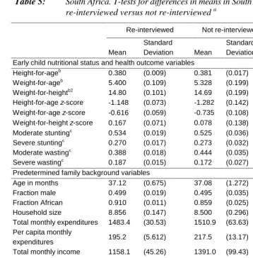
South Africa: Because the South African survey is a comprehensive household survey
with a large number of variables, for comparability this study examined a set of variables similar to those considered for Bolivia, i.e., measures of child nutritional status based on anthropometrics, as well as a set of predetermined family background characteristics. The results reported here cannot, therefore, be immediately generalized to other outcome variables available in the South African data.
Table 3: Bolivia. T-tests for differences in means in Bolivia 1 data for attritors versus nonattritors a
Re-interviewed Not re-interviewed Difference
Variables Mean
Standard
Deviation Mean
Standard
Deviation Mean t-test
Early child development outcome variables Height-for-ageb
18.0 (22.5) 17.4 (22.1) 0.65 (0.72) Weight-for-ageb
32.2 (26.5) 30.3 (25.8) 1.91* (1.81) Weight-for-heightb
58.1 (26.5) 56.9 (27.2) 1.21 (1.10) Moderate stuntingc 0.639 (0.48) 0.631. (0.48) 0.008 (0.43) Severe stuntingc
0.279 (0.45) 0.323 (0.47) -0.0437** (-2.37) Moderate wastingc
0.365 (0.48) 0.400) (0.49 -0.035* (-1.79) Severe wastingc
0.0796 (0.27) 0.0946 (0.29) -0.0150 (-1.30) Gross motor ability 20.8 (7.81) 20.3 (7.67) 0.5136* (1.65) Fine motor ability 19.4 (7.28) 19.0 (7.19) 0.480* (1.65) Language-audition 19.2 (7.62) 18.6 (7.44) 0.569* (1.88) Personal-social 19.9 (8.02) 19.4 (8.06) 0.534* (1.65)
Predetermined family background variables
Mother’s age 29.8 (6.45) 28.7 (6.44) 1.07** (4.10) Father’s age 33.0 (7.70) 32.2 (8.03) 0.85** (2.66) Mother’s schooling 3.0 (1.5) 3.0 (1.5) -0.06 (-0.9113) Father’s schooling 3.6 (1.4) 3.6 (1.4) -0.02 (-0.42) Quechua mainly .00099 (0.0315) 0.0114 (0.106) -0.00414** (-2.85) Amarya mainly .00396 (0.0628) 0.00456 (0.07) -0.000605 (-0.23) Home ownership 0.428 (0.495) 0.215 (0.411) 0.213** (12.02) Number of rooms in house 1.50 (1.05) 1.40 (1.00) 0.100** (4.17) Both parents present 0.841 (0.366) 0.775 (0.42) 0.0656** (4.54) Number of siblings 2.37 (1.80) 2.05 (1.59) 0.322** (4.80) Ownership of durablesd 6.30 (2.11) 5.92 (1.92) 0.375** (4.69) Job of mothere
2.26 (0.91) 2.08 (0.91) 0.174** (4.73) Job of father 2.70 (0.54) 2.70 (0.55) -0.006 (-0.28) Household income 922 (755) 868 (638) 54** (2.68)
Notes: * indicates significance at the 10 percent level, and ** at the 5 percent level.
a
Values of two-sample t-test with unequal variances are given in parentheses in last column.
b
Height-for-age in centimeter/years. Weight-for-age in kilogram/years. Weight-for-height in kilograms/meters.
c
Stunting and wasting are based on height-for-age and weight-for-age. Z-scores calculated are based on CHS/CDC/WHO standards. "Moderate" refers to being more than one standard deviation below the means and "severe" more than two standard deviations below mean.
d
Ownership of durables measures number of durables owned out of 15 asked.
e
Table 4: (Men) Kenya. T-tests for differences in means in Kenya 1 data for those re-interviewed versus not re-re-interviewed a
Re-interviewed Not re-interviewed Difference
MEN:
Variables Mean
Standard
Deviation Mean
Standard
Deviation Mean t-test
Fertility-related outcome variables
Currently using contraceptives 0.196 (0.017) (0.031) -0.033 (-0.95) Ever used contraceptives 0.233 (0.018) 0.311 (0.052) -0.077* (-1.79) Want no more children 0.208 (0.017) 0.237 (0.031) -0.029 (-0.83) Number of surviving children 4.76 (0.171) 3.94 (0.277) 0.817** (2.46)
Family planning program variables
Visited by community-based distribution agent
0.156 (0.015) 0.132 (0.025) 0.024 (0.78)
Heard family planning message on radio 0.931 (0.011) 0.968 (0.013) -0.037* (-1.86) Heard about family planning at clinic 0.495 (0.021) 0.513 (0.036) -0.018 (-0.42) Discussed with others family planning lecture
heard at clinic
0.679 (0.029) 0.691 (0.047) -0.012 (-0.21)
Number of network partners in network for
Family planning 3.7 (0.20) 4.0 (0.35) -0.3 (-0.86) Wealth flows 5.0 (0.21) 5.0 (0.36) -0.04
Reproductive health – – – (-0.10)
Knows secret contraceptive user 0.637 (0.069) 0.558 (0.095) 0.079 (0.60)
Control variables
Age (years) 40.1 (0.52) 36.8 (0.78) 3.3** (3.24) Education
No schooling 0.112 (0.013) 0.063 (0.018) 0.049* (1.94) Some primary schooling 0.577 (0.021) 0.537 (0.036) 0.040 (0.96) Secondary schooling 0.298 (0.019) 0.379 (0.035) -0.081** (-2.06) Language
Luo only 0.796 (0.017) 0.805 (0.029) -0.010 (-0.28) English 0.443 (0.021) 0.532 (0.036) -0.089** (-2.11) Swahili 0.655 (0.020) 0.726 (0.032) -0.072* (-1.82) Lived
outside of province 0.591 (0.021) 0.653 (0.035) 0.061 (1.49) in Nairobi or Mombasa 0.336 (0.020) 0.400 (0.036) -0.064 (-1.58) Belongs to credit group 0.257 (0.019) 0.242 (0.031) 0.015 (0.40) Belong to clan welfare society 0.868 (0.014) 0.905 (0.021) -0.037 (-1.35)
Women sell on market – – –
Household characteristics
Polygamous household 0.293 (0.019) 0.238 (0.031) 0.055 (1.45) Self/Husband receives monthly salary 0.170 (0.016) 0.255 (0.032) -0.085** (-2.56)
Husband interviewed – – –
Household has radio – – –
House has metal roof 0.173 (0.016) 0.189 (0.029) -0.016 (-0.51) Sublocation of residence
Table 4: (continued) (Women)
Re-interviewed Not re-interviewed Difference
WOMEN:
Variables Mean
Standard
Deviation Mean
Standard
Deviation Mean t-test
Fertility-related outcome variables
Currently using contraceptives 0.126 (0.012) 0.103 (0.021) 0.024 (0.91) Ever used contraceptives 0.238 (0.016) 0.196 (0.027) 0.042 (1.25) Want no more children 0.351 (0.018) 0.220 (0.037) 0.132** (3.59) Number of surviving children 3.88 (0.089) 2.78 (0.138) 1.10** (5.90)
Family planning program variables
Visited by community-based distribution agent
0.163 (0.014) 0.113 (0.022) 0.050* (1.75)
Heard family planning message on radio 0.870 (0.916) 0.916 (0.019) -0.046* (-1.79) Heard about family planning at clinic 0.851 (0.013) 0.828 (0.027) 0.023 (0.80) Discussed with others family planning lecture
heard at clinic
0.629 (0.070) 0.661 (0.037) -0.032 (-0.76)
Number of network partners in network for
Family planning 2.9 (0.11) 3.1 (0.20) -.18 (-0.78) Wealth flows 2.8 (0.12) 2.4 (0.21) 0.38 (1.45) Reproductive health 3.2 (0.16) 2.8 (0.23) 0.38 (1.19) Knows secret contraceptive user 0.408 (0.02) 0.377 (0.03) 0.030 (0.77)
Control variables
Age (years) 29.7 (0.332) 26.3 (0.488) 3.4** (5.04) Education
No schooling 0.214 (0.015) 0.141 (0.024) 0.072* (2.30) Some primary schooling 0.669 (0.018) 0.668 (0.033) 0.001 (0.03) Secondary schooling 0.117 (0.012) 0.190 (0.027) -0.074** (-2.75) Language
Luo only 0.422 (0.018) 0.327 (0.033) 0.095* (2.46) English 0.178 (0.014) 0.263 (0.031) -0.086** (-2.73) Swahili 0.396 (0.018) 0.517 (0.035) -0.121** (-3.11) Lived
outside of province 0.370 (0.018) 0.371 (0.034) -0.001 (-0.02) in Nairobi or Mombasa 0.214 (0.015) 0.205 (0.028) 0.009 (0.29) Belongs to credit group 0.351 (0.018) 0.288 (0.032) 0.064* (1.70) Belong to clan welfare society 0.747 (0.016) 0.644 (0.034) 0.103** (2.93) Women sell on market 0.464 (0.019) 0.444 (0.035) 0.020 (0.51) Household characteristics
Polygamous household 0.350 (0.018) 0.371 (0.034) -0.021 (-0.56) Self/Husband receives monthly salary 0.334 (0.019) 0.402 (0.037) -0.068* (-1.66) Husband interviewed 0.765 (0.016) 0.752 (0.029) 0.013 (0.41) Household has radio 0.492 (0.019) 0.546 (0.035) -0.055 (-1.38) House has metal roof 0.201 (0.015) 0.187 (0.027) 0.014 (0.45) Sublocation of residence
Gwassi 0.213 (0.015) 0.210 (0.029) 0.003 (0.08) Kawadhgone 0.240 (0.015) 0.205 (0.028) 0.035 (1.06) Oyugis 0.286 (0.017) 0.263 (0.031) 0.023 (0.63) Ugina 0.261 (0.016) 0.322 (0.033) -0.061* (-1.72)
Note:
* indicates significance at the 10 percent level, and ** at the 5 percent level.
a
Table 5: South Africa. T-tests for differences in means in South Africa 1 data for those re-interviewed versus not re-interviewed a
Re-interviewed Not re-interviewed Difference
Mean
Standard
Deviation Mean
Standard
Deviation Means t-test Early child nutritional status and health outcome variables
Height-for-ageb 0.380 (0.009) 0.381 (0.017) -0.001 (-0.08)
Weight-for-ageb 5.400 (0.109) 5.328 (0.199) 0.072 (0.32)
Weight-for-heightb2 14.80 (0.101) 14.69 (0.199) 0.111 (0.50)
Height-for-age z-score -1.148 (0.073) -1.282 (0.142) 0.134 (0.84) Weight-for-age z-score -0.616 (0.059) -0.735 (0.108) 0.119 (0.97) Weight-for-height z-score 0.167 (0.071) 0.078 (0.138) 0.090 (0.58) Moderate stuntingc 0.534 (0.019) 0.525 (0.036) 0.008 (0.21)
Severe stuntingc 0.270 (0.017) 0.273 (0.032) -0.002 (-0.07)
Moderate wastingc 0.388 (0.018) 0.444 (0.035) -0.057 (-1.42)
Severe wastingc 0.187 (0.015) 0.172 (0.027) 0.016 (0.51)
Predetermined family background variables
Age in months 37.12 (0.675) 37.08 (1.272) 0.044 (0.03) Fraction male 0.499 (0.019) 0.495 (0.035) 0.004 (0.11) Fraction African 0.910 (0.011) 0.859 (0.025) 0.051* (1.89) Household size 8.856 (0.147) 8.500 (0.296) 0.356 (1.08) Total monthly expenditures 1483.4 (30.53) 1510.9 (63.63) -27.46 (-0.39) Per capita monthly
expenditures 195.2 (5.612) 217.5 (13.17) -22.33 (-1.56) Total monthly income 1158.1 (45.26) 1391.0 (99.43) -234** (-2.13) Per capita monthly income 156.3 (7.922) 216.6 (21.36) -60.4** (-2.65) Household head age 51.77 (0.524) 52.64 (1.095) -0.871 (-0.72) Household head education 2.957 (0.125) 3.485 (0.255) -0.528* (-1.86) Household head male 0.695 (0.017) 0.702 (0.033) -0.007 (-0.18) Own house 0.883 (0.012) 0.838 (0.026) 0.044 (1.53) Number of rooms 4.951 (0.100) 5.318 (0.215) -0.367 (-1.55) Number of durables 3.149 (0.082) 3.556 (0.149) -0.41** (-2.39) Urban 0.289 (0.017) 0.343 (0.034) -0.054 (-1.44) In former Natal 0.165 (0.014) 0.237 (0.030) -0.07** (-2.18)
Notes: * indicates significance at the 10 percent level, and ** at the 5 percent level.
a
Values of two-sample t-test with unequal variances are given in parentheses in last column.
b
Height-for-age in meter/years. Weight-for-age in kilogram/years. Weight-for-height in kilograms/meters.
c
4.2 Probits for Probability of Attrition
We start with a parsimonious specification of probits for the probability of attrition in which only one outcome variable at a time is included; we then include all outcome variables plus predetermined family background variables (Table 6). The dependent variable in these probits is whether attrition occurred between the survey rounds (1=yes; 0=no) 2 tests for the significance of the overall relations are presented at the bottom of Table 6.
Bolivia:7KH 2 tests indicate that if only one of the outcome variables at a time is
included in these probits, the probit is significant at the 5 percent level only for severe stunting, that is, a child who is severely stunted is more likely to be lost to follow-up. For moderate and severe low weight-for-age and the four test scores, the probits are significant at the 10 percent level, suggesting that poor childhood development is associated with higher probability of attrition. When all of the family background variables and all childhood development indicators are included in the analysis, however, among the childhood development indicators only moderate stunting is significantly nonzero, even at the 10 percent level, with a negative sign. That 1 in 11 of the childhood development indicators has a significant coefficient estimate at the 10 percent level in the multivariate analysis is what one would expect to occur by chance, even if none of the childhood development indicator coefficients were truly significant predictors of attrition. Moreover, the one childhood development outcome variable that has a significantly nonzero coefficient estimate in Table 6 in the multivariate analysis does not show significant differences in the comparison of means in Table 3.
D em ographi c Research - Vo lu m e 5 , Ar tic le 4 h ttp ://www. d em o g ra p h ic -r es ea Pr ob its fo r pr edi ct in g a ttr iti o n b et w ee n r o und s 1 a n d 2 f o r Bol iv ian , K en and Sout h Af ri can dat a a All outcome variables + pre-determined variablese 1.204 (1.30) 0.040 (1.02) -0.082 (-1.20) 0.297* (1.67) -0.144 (-0.95) -0.036 (-0.33) 0.005 (0.03) Outcome variables, one at a time
0.016 (0.09) -0.009 (-0.45) -0.005 (-0.34) 0.136 (1.25) -0.062 (-0.52) -0.019 (-0.21) 0.007 (0.06) Outcome variables Height-for-age Weight-for-height Weight-for-age Moderate wasting Severe wasting Moderate stunting Severe stunting All outcome variables + pre-determined variablesd 0.004 (0.02) -0.036 (0.28) -0.010 (0.07) -0.136** (3.73) -0.010 (0.56) Outcome variables, one at a time
-0.134 (0.92) -0.142 (1.26) -0.374** (3.60) -0.139** (5.82) 0.012 (0.78) All outcome variables + pre-determined variablesc -0.065 (0.34) -0.103 (-0.70) 0.245* (1.69) -0.017 (-0.78) 0.003 (0.22) Outcome variables, one at a
time 0.118 (0.95) 0.162* (1.67) 0.099 (0.83) -0.033** (-2.46) -0.009 (-0.85) Outcome variables Currently contracepting Ever used contraceptives
Want no more children Number of surviving children Number of family planning network partners All outcome variables + pre-determined variablesb -.0002 (-0.04) .0032 (0.80) -.0037 (-0.78) .1003 (0.70) .1353 (0.70) -.291* (-1.93) .2066 (1.51) .0123 (0.59) -.0073 (-0.35) -.0059 (-0.27) -.0014 (-0.07) Outcome variables, one at a
Table 6: (notes)
Note: * indicates significance at the 10 percent level, and ** indicates significance at the 5 percent level. a Values of z-tests are in parentheses beneath point estimates. P-values of Chi-square tests are in brackets.
b Predetermined variables for Bolivian households that are: (a) significant at 5 percent level (with sign in parentheses)—father’s age(+); Quechua only (+); ownership of house (-); number of durables owned (-); Oruro (-), Postosi (-), Santa Cruz (-) relative to La Paz; mother’s job permanent relative to no job (-); (b) significant at the 10 percent level – father’s schooling (-), number of rooms in the house (+), number of siblings of child (-); father’s job temporary relative to no job (-); (c) not significant even at the 10 percent level – mother’s age, mother’s schooling, Amarya only, El Alto, Cochabamba, Tarija relative to La Paz; father’s job permanent relative to no job; mother’s job temporary relative to no job; household income.
c Predetermined variables for Kenyan men that are (a) significant at the 5 percent level (with sign in parentheses)—men’s age; (b) not significant even at the 10 percent level – primary schooling; secondary schooling; Luo only; English; lived in Nairobi or Mombasa; polygamous household; earns a monthly salary; sublocation of residence.
d Predetermined variables for Kenyan women that are: (a) significant at the 5 percent level (with sign in parentheses)—husband interviewed (-); (b) significant at the 10 percent level—resided in Oyugnis relative to Ugina (-) (c) not significant even at the 10 percent level—primary schooling; secondary schooling; Luo only; English; lived in Nairobi or Mombasa; polygamous household; household has radio; household has metal roof; other sublocation of residence.
e Predetermined variables for South African households that are (a) significant at the 5 percent level (with sign in parentheses)— age of household head(+); (b) significant at the 10 percent level—none; (c) not significant even at the 10 percent level—male child; African household; household size; ln total monthly expenditures; household head schooling; male household head; own the house; number of rooms; number of durables; urban; former Natal.
I)RU%ROLYLDQGDWD3UREDELOLW\! DDWWKHSHUFHQWOHYHO²VHYHUHVWXQWLQJEDWWKHSHUFHQWOHYHO²ZHLJKWIRUDJH
moderate wasting, language-auditory.
J)RU.HQ\DQPHQ3UREDELOLW\! DDWWKHSHUFHQWOHYHO²QXPEHURIVXUYLYLQJFKLOGUHQEDWWKHSHUFHQWOHYHO²HYHUXVHG
contraceptives.
K)RU.HQ\DQZRPHQ3UREDELOLW\! DDWWKHSHUFHQWOHYHO²ZDQWQRPRUHFKLOGUHQQXPEHURIVXUYLYLQJFKLOGUHQ
i)RU6RXWK$IULFDQGDWD3UREDELOLW\!2
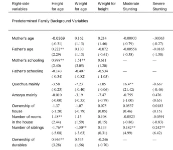
percent level) associated with higher probability of attrition: older and less-schooled fathers, speaking mainly Quechua in the household, not owning the home, having more rooms in the house, having fewer siblings, having fewer durables, father having permanent or no (rather than a temporary) job, and mother having no or a temporary (rather than a permanent) job, with some significant differences also among the urban areas included in the program. The majority of these significant coefficient estimates are consistent with what might be predicted from the significant differences in the means in Table 3, reinforcing the observation that attrition tends to be selectively greater among children from worse-off family backgrounds.
But some of these significant coefficient estimates are opposite in sign from what might be expected from the comparisons of the means in Table 3, suggesting the opposite relation to attrition if there are multivariate controls for standard background variables other than what appear in the comparisons of means. Specifically, the comparisons in Table 3 suggest that attrition is significantly more likely if fathers are younger, the house has fewer rooms, and there are fewer siblings, but all three of these signs are reversed with significant coefficient estimates in the multivariate analyses of Table 6. Moreover, two variables that are not significantly different for the two subsamples in Table 3 have significant coefficient estimates in Table 6, i.e., father’s schooling and father having a temporary job, both of which are estimated to significantly reduce attrition probabilities in Table 6. Finally, both mother’s age and household income have means that are significantly different between the subsamples in the univariate comparisons in Table 3, but do not have coefficient estimates that are significantly nonzero, even at the 10 percent level, once there is control for other family background characteristics in Table 6.
Thus, exactly which family background characteristics predict attrition with multivariate controls and what the directions of those effects are cannot be inferred simply by examining the significance of means in univariate comparisons between the subsamples. While the patterns in Tables 3 and 6 suggest that worse-off family background is associated with greater attrition, the multivariate estimates are less supportive of this conclusion.
Kenya: Since there are gender differences in the probit estimates of the probability of
attrition, we report separately for men and women (Table 6). For men, we find that when the five outcomes are included singly, only the number of surviving children is significantly related to attrition at the 5 percent level; one other – ever-used family planning – is significantly related to attrition at the 10 percent level. If other right-side variables are included, among the five fertility related outcomes none is significantly nonzero at the 5 percent level, and only not wanting more children is significantly related to attrition at the
SHUFHQWOHYHO$ 2 test for the joint significance of these five variables rejects such
current VXEORFDWLRQRIUHVLGHQFH$ 2 test for the joint significance of all the right-side variables rejects such significance at the 5 percent level (p=0.068).
For women, we find that two of the lagged outcome variables, wanting no more children and the number of surviving children, are individually significant (and negative). When all the lagged outcome variables and the predetermined variables are included, only the latter (number of surviving children) remains significant. However, in contrast to the
UHVXOWV IRU PHQ 2 tests for the joint significance of the five fertility related outcome
variables and for the entire set of right-side variables indicate significance (p < 0.0001 in both cases).
Thus, for the Kenyan data, there is no significant association between attrition, most of the outcome variables, and most of the major control variables. However, gender does matter in these multivariate analyses: there is a significant negative association between attrition and number of surviving children for women but not for men.
South Africa: Probit estimates for the probability of attrition reveal little evidence that
the outcome variables are associated with attrition of pre-school children, paralleling the results of the mean comparisons presented in Section 4.1. When only one outcome variable at a time is included, none is significant at conventional levels. When the set of outcome variables are included at the same time, all but moderate wasting are insignificant and a
MRLQW 2 test indicates that the set of all outcome variables together is insignificant.
Moreover, the overall relation is insignificant – this set of background characteristics and outcome variables does a very poor job predicting attrition in the sample. Thus, for the South African data, there is no significant association between attrition of pre-school children, most of the outcome variables, and most of the major control variables.
4.3 Do Those Lost to Follow-up have Different Coefficient Estimates than Those Re-interviewed?
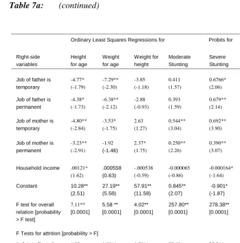
Our aim here is to determine whether those who subsequently leave the sample differ in their initial behavioral relationships. We conduct the BGLW tests, in which the value of an outcome variable at the initial wave of the survey is regressed on predetermined variables for the initial survey wave and on subsequent attrition. In short, the test is whether the coefficients of the predetermined variables and the constant differ for those respondents who are subsequently lost to follow- up versus those who are re-interviewed. Tables 7, 8, and 9 present these multivariate regression and probit estimates for the same outcome variables considered above, with the same family background variables as controls. The first part of each table gives the coefficient estimates for the family background variables for the subsample of those who were re-interviewed. At the bottom of each table are the F
are significant differences between the two subsamples that test for equality of (i) all of the slope coefficients and the constant and (ii) all of the slope coefficients (but not the constant).
Bolivia: F tests indicate that all of the eleven estimated equations for childhood
development indicators are statistically significant with a p-value of p < 0.0001 (Table 7). These estimates indicate a number of associations that are consistent with widely held perceptions about child development. For example, household income is significantly positively associated with height-for-age and significantly negatively associated with severe stunting; mother’s schooling is significantly positively associated with height-for-age and weight-for-age, though significantly negatively associated with gross motor ability; and ownership of consumer durables is significantly positively associated with height-for-age, gross motor ability, fine motor ability, language-audition, and personal-social test scores, but significantly negatively associated with severe wasting.
There are, however, no significant differences at the 5 percent level (Note 15) between the set of coefficients for the subsample of those lost to follow-up versus the subsample of those re-interviewed for over half of the indicators of child development: height-for-age, moderate stunting, gross motor ability tests, fine motor ability tests, language-audition tests, and personal-social tests. The second set of tests, further, indicates that there are no significant differences at the 10 percent level for severe stunting. These estimates for the anthropometric indicators related to stunting and for the four cognitive development test scores, therefore, suggest that the coefficient estimates of standard family background variables are not significantly affected by sample attrition.
The results differ sharply, however, for the anthropometric indicators related to wasting. Both tests for these four child outcome variables indicate that the coefficient estimates for observed family background variables do differ significantly at the 5 percent level (and for all but weight-for-age at the 1 percent level) between the two subsamples. For these outcomes, therefore, it is important to control for the attrition in the analysis, e.g., as with the matching methods used in Behrman, Cheng and Todd (2001).
Kenya: We conduct BGLW tests with Kenya 1 contraceptive use (ever or current),
for currently using contraceptives, both only for women and in both of which cases the constant differs between the subsamples, but not the slope coefficient estimates).
Thus there is no significant effects on the slope coefficients of attrition for either men or women, and but limited evidence of a significant effect on the constants for women.
South Africa: The evidence for South Africa presented earlier in Sections 4.1 and 4.2
suggests that attrition bias resulting from selection on observables is not present. The BGLW tests examined in this section largely confirm this, although there are some exceptions.
For the first three anthropometric outcomes shown in Table 9, the attrition interactions are not jointly significant with or without the attrition dummy variable. In the remaining columns that present the stunting and wasting probits, the attrition interaction terms are significant only in the case of moderate stunting, indicating the possibility of attrition bias in this relationship. On the other hand, attrition does not appear to have any association with severe stunting or moderate and severe wasting.
As described in Section 3, one important difference in the South African sample relative to the others is that, when possible, households that had moved were followed. These households are included in the analysis presented above. What would happen if they were excluded? Re-estimating the equations in Table 9 categorizing those who had moved but were interviewed as if they had been lost to follow-up and not re-interviewed leads to a somewhat stronger, but still fairly weak, rejection of the null hypothesis that there are no differences in coefficients across the two groups (results not shown). In every case the
p-YDOXHVIRUHLWKHUWKH)RU 2 tests on the attrition interactions decline; for height-for-age,
Table 7a: Bolivia. Testing impact of attrition between Bolivia 1 and Bolivia 2 on coefficient estimates of family background variables in early childhood
development anthropometric outcomesa
Ordinary Least Squares Regressions for Probits for
Right-side variables Height for age Weight for age Weight for height Moderate Stunting Severe Stunting Moderate Wasting Severe Wasting
Predetermined Family Background Variables
Mother’s age -0.0369
(-0.31) 0.162 (1.13) 0.214 (1.46) -0.00933 (-0.79) -.00363 (-0.27) -0.00352 (-0.29) 0.0142 (0.67)
Father’s age 0.222** (2.29) 0.130 (1.13) -0.072 (-0.61) -0.00558 (-0.58) -0.0165 (-1.50) -.0209** (-2.08) -0.0186 (-1.06)
Mother’s schooling 0.998** (2.40) 1.51** (3.05) 0.611 (1.20) — — — —
Father’s schooling -0.143 (-0.34)
-0.407 (-0.82)
-0.534 (-1.05)
— — — -0.106
(-1.37)
Quechua mainly -3.58 (-0.23) -7.23 (-0.40) -1.05 (-0.06) 16.4** (21.42) -0.667 (-0.46) 17.3** (25.26) —
Amarya mainly -0.010 (-0.00) -3.19 (-0.35) -7.47 (-0.79) -0.755 (-1.00) 0.476 (0.65) 0.313 (0.43) — Ownership of house -1.37 (-1.20) -1.07 (-0.79) 0.075 (0.05) 0.0537 (0.46) 0.0183 (0.15) -0.0225 (-0.20) —
Number of rooms in the house
1.48** (2.44) 1.15 (1.59) 0.108 (0.15) -0.0523 (-0.86) -0.0591 (-0.83) -0.0127 (-0.21) -0.0269 (-0.23)
Number of siblings -1.76** (-5.08) -1.50** (-3.63) 0.133 (0.31) 0.182** (4.99) 0.242** (6.42) 0.104** (3.00) — Ownership of durables 0.946** (3.28) 0.535 (1.56) -0.246 (-0.70)
— — — -0.172**
(-3.13)
El Alto 0.036 (0.03) -0.135 (-0.08) 2.149 (1.182) .262* (1.70) 0.343** (2.22) -0.0610 (-0.42) -0.150 (-0.54) Cochabamba 4.63** (2.94) -2.17 (-1.16) -6.01** (-3.12)
— — 0.130
(0.84) — Oruro -4.43** (-2.10) -6.89** (-2.75) 1.12 (0.44) 0.526** (2.29) 0.551** (2.56) 0.509** (2.53) 0.676** (2.10) Potosi -0.869 (-0.43) -10.0** (-4.16) -11.93** (-4.83) 0.229 (1.08) 0.481** (2.34) 0.936** (4.78) — Tarija 6.65** (3.18) 14.35** (5.76) 12.4** (4.83) -0.189 (-0.91) -0.0944 (-0.41) -0.723** (-3.10) —
Table 7a: (continued)
Ordinary Least Squares Regressions for Probits for
Right-side variables Height for age Weight for age Weight for height Moderate Stunting Severe Stunting Moderate Wasting Severe Wasting
Job of father is temporary -4.77* (-1.79) -7.29** (-2.30) -3.85 (-1.18) 0.411 (1.57) 0.6766* (2.06) 0.372 (1.35) —
Job of father is permanent -4.38* (-1.73) -6.38** (-2.12) -2.88 (-0.93) 0.393 (1.59) 0.679** (2.14) 0.282 (1.07) 0.0729 (0.16)
Job of mother is temporary -4.80** (-2.84) -3.53* (-1.75) 2.63 (1.27) 0.544** (3.04) 0.692** (3.90) 0.268* (1.61) 0.0967 (0.33)
Job of mother is permanent -3.23** (-2.91) -1.92 (-1.46) 2.37* (1.75) 0.250** (2.26) 0.390** (3.07) 0.226** (2.01) 0.0356 (0.18)
Household income .00121* (1.62) .000558 (0.63) -.000538 (-0.59) -0.000065 (-0.86) -0.000164* (-1.64) -0.0000262 (-0.33) -0.0000376 (-0.25) Constant 10.28** (2.51) 27.19** (5.58) 57.91** (11.58) 0.845** (2.07) -0.901* (-1.87) -0.00232 (-0.01) -1.39* (-1.91)
F test for overall relation [probability > F test]
7.11** [0.0001] 5.58 ** [0.0001] 4.02** [0.0001] 257.80** [0.0001] 278.38** [0.0001] 179.06** [0.0001] 98.91** [0.0001]
F Tests for attrition [probability > F]
1. Joint effect of attrition on constant and all estimates 1.32 [0.1428] 1.88** [0.0070] 1.58** [0.0385] 22.68 [0.3614] 35.34* [0.0357] 44.86** [0.0018] 261.66** [0.0001]
2. Joint effect of attrition on all coefficient estimates but not on constant 1.37 [0.1169] 1.90** [0.0068] 1.63** [0.0315] 22.49 [0.3147] 29.18 [0.1097] 42.17** [0.0026] 253.89** [0.0001] Note:
* indicates significance at the 10 percent level, and ** indicates significance at the 5 percent level. P-values of tests are in brackets.
a
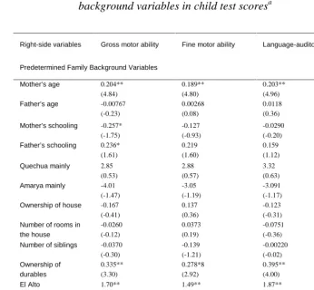
Table 7b: Bolivia. Multivariate ordinary least squares regressions for testing impact of attrition between Bolivia 1 and Bolivia 2 on coefficient estimates of family background variables in child test scoresa
Right-side variables Gross motor ability Fine motor ability Language-auditory Personal-social
Predetermined Family Background Variables
Mother’s age 0.204** (4.84) 0.189** (4.80) 0.203** (4.96) 0.199** (4.57)
Father’s age -0.00767 (-0.23) 0.00268 (0.08) 0.0118 (0.36) 0.00547 (0.16)
Mother’s schooling -0.257* (-1.75) -0.127 (-0.93) -0.0290 (-0.20) -0.167 (-1.10)
Father’s schooling 0.236* (1.61) 0.219 (1.60) 0.159 (1.12) 0.209 (1.38)
Quechua mainly 2.85 (0.53) 2.88 (0.57) 3.32 (0.63) 4.28 (0.77)
Amarya mainly -4.01 (-1.47) -3.05 (-1.19) -3.091 (-1.17) -2.91 (-1.03)
Ownership of house -0.167 (-0.41) 0.137 (0.36) -0.123 (-0.31) —
Number of rooms in the house -0.0260 (-0.12) 0.0373 (0.19) -0.0751 (-0.36) 0.0433 (0.20)
Number of siblings -0.0370 (-0.30) -0.139 (-1.21) -0.00220 (-0.02) -0.103 (-0.81) Ownership of durables 0.335** (3.30) 0.278*8 (2.92) 0.395** (4.00) 0.403** (3.84)
El Alto 1.70** (3.26) 1.49** (3.07) 1.87** (3.71) 1.84** (3.43) Cochabamba 0.569 (1.03) -0.254 (-0.49) 0.156 (0.29) 0.675 (1.18) Oruro .537 (0.72) -0.337 (-0.49) 0.761 (1.06) 0.401 (0.52) Potosi -1.08 (-1.51) -1.23* (-1.85) -0.720 (-1.04) -1.07 (-1.45) Tarija 4.01** (5.43) 2.64** (3.83) 3.31** (4.63) 3.68** (4.83)
Table 7b: (continued)
Right-side variables Gross motor ability Fine motor ability Language-auditory Personal-social
Predetermined Family Background Variables
Job of father is temporary — -1.79* (-2.05)
-1.77* (-1.95)
-1.69* (-1.75)
Job of father is permanent -2.35** (-2.64) -2.03** (-2.44) -2.09** (-2.42) -2.02** (-2.20)
Job of mother is temporary 2.20** (3.69) 1.92** (3.45) --- 2.17** (3.53)
Job of mother is permanent 0.948** (2.43) 0.900** (2.45) 0.844** (2.22) 1.06** (2.63)
Household income .000068 (0.26) .0000878 (0.36) -0.0000282 (-0.11) -0.0000404 (-0.15) Constant 13.4** (9.28) 12.47 ** ( 9.25) 10.28** (7.35) 11.4** (7.62)
F-test for overall relation [probability > F-test]
5.38** [0.0001] 5.21** [0.0001] 5.80** [0.0001] 5.39** [0.0001]
F-Tests for Attrition [probability > F]
1. joint effect of attrition on all estimates, including constant 1.31 [0.1461] 1.45* [0.0772] 1.34 [0.1277] 1.38 [0.1055]
2. joint effect of attrition on all coefficients but not on constant 1.37 [0.1160] 1.51* [0.0594] 1.40 [0.1013] 1.44* [0.0824] Note:
* indicates significance at the 10 percent level, and ** indicates significance at the 5 percent level. P-values of tests are in brackets.
a