Global error estimation of linear multistep methods through the Runge-Kutta methods

Galley

Pro

of

Global error estimation of linear

multistep methods through the

Runge-Kutta methods

J. Farzi∗

Abstract

In this paper, we study the global truncation error of the linear multi-step methods (LMM) in terms of local truncation error of the corresponding Runge-Kutta schemes. The key idea is the representation of LMM with a cor-responding Runge-Kutta method. For this, we need to consider the multiple step of a linear multistep method as a single step in the corresponding Runge-Kutta method. Therefore, the global error estimation of a LMM through the Runge-Kutta method will be provided. In this estimation, we do not take into account the effects of roundoff errors. The numerical illustrations show the accuracy and efficiency of the given estimation.

Keywords: Linear multistep methods; Runge-Kutta methods; Local

trun-cation error; Global error; Error estimation.

1 Introduction

The error estimation is one of the major issues in designing numerical algo-rithms. In the study of the linear multistep methods (LMM)

k

∑

j=0

αjyn+j =h k

∑

j=0

βjfn+j, (1)

for solving an ordinary differential system {

y′=f(x, y), y(x0) =y0,

(2) where,f :R×Rm_→Rm_{, there is a challenging issue of estimation of global}

truncation error (GTE) or simply global error. In spite the local trunca-tion error (LTE), the estimatrunca-tion of GTE is much more complicated. The

∗_{Corresponding author}

Received 25 December 2015; revised 9 March 2016; accepted 11 2016 J. Farzi

Department of Mathematics, Sahand University of Technology, P.O. Box 51335-1996, Tabriz, Iran. e-mail: [email protected]

Galley

Pro

of

100 J. Farzi

LTE estimations have been studied in some special cases, e.g., predictor-corrector (PC) and embedded Runge-Kutta methods. In the case of PC methods that predictor is an Adams-Bashforth scheme of order p and cor-rector is an Adams-Moulton scheme of the same order, the Milne estimation provides an estimation for LTE of the resulted PC method [9, 10]. Recently, Cao and Petzold have developed an estimation for global error with adjoint method [3]. However, many efforts have previously been reported for provid-ing GTE bounds [6, 7]. These bounds are of no practical value and the LTE form estimation of GTE, given in this paper, is more simpler than the usual theoretical bounds. For more extensive discussion on linear multistep meth-ods and their important subclauses, like backward difference formula (BDF) schemes see [1, 2, 8–10, 12]. The more important application of the LMMs is in the time discretization of time dependent partial differential equations. The LMMs with strong stability preserving property (SSP) have a major role in this context [4, 5].

In this paper, we represent a multiple step of a LMM as a single step of a new Runge-Kutta method. Then, we accomplish the GTE estimation of the LMM by estimation of LTE of the corresponding new Runge-Kutta method. This paper has been organized as follow: In Section 2 a very short review of the Runge-Kutta schemes is presented. Then, in Section 3 the main idea of the paper is given for one-step methods with a rather detailed study of the LTE and stability region of the new method. In Section 4 the idea of previous section is generalized to formulate a general LMM in the form of a new Runge-Kutta method. The new RK method has a popular structure in view of Butcher array. We take into account a starting procedure, subsequently, the method order and its LTE determined, which is the GTE of the original scheme. Finally, in Section 5 we present some numerical tests including a fourth order total variation bounded (TVB) scheme to illustrate efficiency of the given theory.

2 A review of Runge-Kutta methods

In this section, we shortly review the main concepts of Runge-Kutta methods that are required in the rest of the paper. For more details we refer to [2, 9]. Thes-stage Runge-Kutta method for the problem (2) is defined as follow

yn+1=yn+h s

∑

i=1

biki, (3)

where

ki=f(xn+cih, yn+h s

∑

j=1

Galley

Pro

of

c A

bT (5)

where,

c= [c1, c2, . . . , cs]T, b= [b1, b2, . . . , bs]T, A= [aij]si,j=1. (6) The derivation of a Runge-Kutta method of an arbitrary order is a crucial work without using the advanced concepts of elementary differentials and most related rooted trees. In fact, there is a 1-1 corresponding between ele-mentary differential (that are defined by Fr´echet derivative) and the rooted trees. Therefore, using the rooted trees one can easily define the order con-dition and LTE of a Runge-Kutta method. The local truncation error of the

pth _{order Runge-Kutta method (5) is given by}

LTE = h

p+1 (p+ 1)!

∑

r(t)=p+1

α(t)[1−γ(t)ψ(t)]F(t) +O(hp+2), (7) where,

α(t) = r(t)!

σ(t)γ(t)

and r(t), σ(t) and γ(t) are order, symmetry and density of a tree t. The functionF(t) is defined on the setT of all trees which corresponds between the rooted trees and elementary differentials. The elementary differentials are evaluated at the valuey(xn). Theψ(t) function is also defined on the set

of all treesT. For example we have,

F( ) =f,

F( ) ={f}=f(1)(f),

F( ) ={f2}=f(2)(f, f),

F( ) ={2f}2=f(1)(f(1)(f)),

where, f(M)(K1, K2, . . . , KM), Kt ∈ Rm, t = 1,2, . . . , M is theMth order

Galley

Pro

of

102 J. Farzi

The following theorem gives the coefficients of the linear combination of

y(q)_{for a generalqin terms of elementary differentials [9]:}

Theorem 1. Let y be the solution of the autonomous problem (1). Then

y(q)= ∑

r(t)=q

α(t)F(t). (8)

The stability function of a Runge-Kutta method is given by

R(ˆh) =det [I− ˆ

hA+ ˆhebT_]

det [I−ˆhA] , (9)

where, ˆh=λh, hereλis typically an eigenvalue of the jacobian matrix off

that is equivalently the eigenvalues of the linearized equation.

3 One step methods

In this section, we firstly study the situation for the one-step methods. The idea will be extended to a general linear multistep methods in the next sec-tions. Consider the following linear one step method

yn+1=yn+h(β0fn+β1fn+1) (10)

for a consistent method we haveβ0+β1= 1. Applying the above rule onN successive steps to advance the solution from x0 toxN we obtain

y1 =y0+h(β0f0+β1f1)

y2 =y1+h(β0f1+β1f2) ..

.

yN =yN−1+h(β0fN−1+β1fN).

Introducing the following slopes

k1=f(x0, y0), k2=f(x1, y1), . . . , kN+1=f(xN, yN),

we can write (10) as a (N+1)-stage Runge-Kutta method with the steplength

H =N h,

ym+1 =ym+

H

N(β0k1+k2+· · ·+kN +β1kN+1)

Galley

Pro

of

k1=f(tm, ym)

k2=f(tm+

H N, ym+

H

N(β0k1+β1k2))

.. .

kN+1=f(tm+H, ym+

H

N(β0k1+k2+· · ·+kN+β1kN+1)).

Thus, the corresponding Butcher array takes the following form 0 0 1 N β0 N β1 N 2 N β0 N 1 N β1 N .. . ... ... . .. N N β0 N 1

N · · ·

1 N β1 N β0 N 1

N · · ·

1

N β1

N

(11)

3.1 Local truncation error

In this section we obtain the LTE and the order of the reduced method (11). To determine the order of the deduced RK scheme we verify the order conditions for the Butcher array (11):

ψ( ) =

N_∑+1

i=1

bi= 1, (12)

ψ( ) =

N∑+1

i=1

bici=

1

2. (13)

Since we have β0+β1 = 1, substituting the data from (11) we observe that the first condition always holds

N_∑+1

i=1

bi = 1⇒

β0

N +

1

N +· · ·+

1

N +

β1

N = 1.

However, for the second condition to be valid we have,

β0

N.0 +

1

N(

1

N +

2

N +· · ·+

N−1

N ) +

β1

N. N N

= N

2_{−N+ 2β} 1N

2N2 =

1

Galley

Pro

of

104 J. Farzi

where, we have usedβ0+β1= 1. Therefore, the only possible second order one step method is the trapezoidal rule.

Now, we can find the general form of the local truncation error for both first (forward and backward euler) and second order (Trapezoidal) methods.

For the second order method we have,β1=1₂,

ψ( t1= ) =

N∑+1

i=1

bic2i =

2N2_{+ 1} 6N2 ,

ψ(t2= ) =

N_∑+1

i,j=1

biaijcj=

1

N[

1

2,1, . . . ,1, 1 2]Ac=

2N2+ 1 12N2 .

It is evident that in the limit the above order conditions, asN → ∞, tend to the following infinite dimensional exact order conditions:

∞

∑

i=1

bic2i =

1 3,

∞

∑

i,j=1

biaijcj =

1 6.

The corresponding elementary differentials with the rooted trees t1 and

t2are,

F(t1) =f(2)(f, f), F(t2) =f(1)(f(1)(f)).

To specify the LTE of second order scheme we need a representation of y(3) in terms of elementary differentials. According to Theorem 1, we have

y(3)=F(t1) +F(t2), (14)

therefore, the principle term in local truncation error (PLTE) for β1 = 12, wherep= 2 reads

PLTE = H 3 3!

∑

r(t)=3

α(t)[1−γ(t)ψ(t)]F(t) (15)

= H 3 3! (−

1

2N2)(F(t1) +F(t2)) =−1

12N h

3_y(3)_(x0) =−1

12h 2

(xN−x0)y(3)(x0),

Galley

Pro

of

12h 2_(x

N −x0)y(3)(x0) +O(h3). (16) We can also regard (16) as the global error inN steps of the trapezoidal rule. Similarly, forβ1̸=1₂ we obtain

LTE = 1

2N(N−1 + 2β1)h 2_y(2)_(x

0) +O(h3). (17)

3.2 Stability regions

To construct the stability function of (11) we simply note that

ˆ HA= ˆ H N     

β0β1 . ._.

β01 . . .1 β1    

, Hebˆ T = ˆ H N     

β01. . .1β1

β01 1β1

..

. ... ... ...

β01. . .1β1     ,

thus we have

I−HAˆ + ˆHebT =        

1 + ˆHβ0

N

ˆ

H

N . . .

ˆ

H N

ˆ

H Nβ1

1 + ˆHβ0

N ˆ H N ˆ H Nβ1

. ._. .._. 1 + ˆHβ0

N

ˆ

H Nβ1 1         , and thereby,

det[I−HAˆ + ˆHebT] = (1 + ˆHβ0

N)

N_.

Similarly, we can show that the following relation is also valid det[I−HAˆ ] = (1−Hˆβ1

N)

N_.

Inserting the above results into (9) we obtain

R( ˆH) = (1 + ˆH

β0

N) N

(1−Hˆβ1

N)N

. (18)

Galley

Pro

of

106 J. Farzi

−6 −4 −2 0 2

−4 −3 −2 −1 0 1 2 3 4

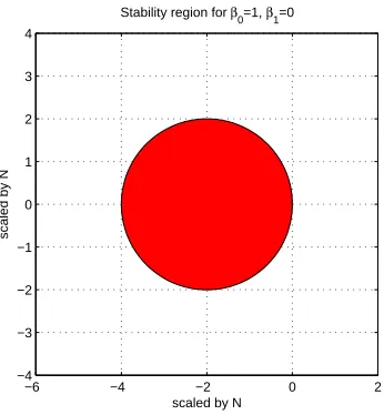
Stability region for β₀=1, β₁=0

scaled by N

scaled by N

Figure 1: The stability region of the new RK method withβ0= 1, β1= 0

−2 −1 0 1 2 3 4 5 6

−4 −3 −2 −1 0 1 2 3 4

Stability region for β₀=0, β₁=1

scaled by N

scaled by N

Galley

Pro

of

−6 −4 −2 0 2

−4 −3 −2 −1 0 1 2 3 4

Stability region for β₀>0, β₁>0 , β₀+β₁=1

scaled by N

scaled by N

Figure 3: The stability region of the new RK method withβ0>0, β1>0, β0+β1= 1

In Figures 1, 2, 3, the absolute stability regions of the given RK method (11) have been demonstrated for various values of β0 and β1. We observe that in the caseβ0>0, β1>0, β0+β1= 1 the new RK method is A-stable and in the cases β0 = 0, β1 = 1 and β0 = 1, β1 = 0 the absolute stability regions, in terms of ˆh, tend to the same regions of the forward and backward Euler methods, respectively.

4 Linear multistep methods

In this section, we present the general theory for an arbitrary linear multistep method. We demonstrated the main idea by using the one-step and multi-step starting procedures. In both cases, we obtain the corresponding Runge-Kutta scheme and the LTE of this method provide an estimation of the global truncation error of the given LMM.

4.1 A single step method as starting procedure

Galley

Pro

of

108 J. Farzi

yn+1=yn+

h

2(fn+fn+1), we find

yn+j=yn+

h

2(fn+ 2fn+1+· · ·+ 2fn+j−1+fn+j), j = 1,2, . . . (19) therefore, we have

k

∑

j=0

αjyn+j=yn+k+ ( k₋1 ∑

j=0

αj)yn+

h

2{(

k₋1 ∑

j=1

αj)fn+ (α1+ 2

k₋1 ∑

j=2

αj)fn+1 +· · ·+ (αk−2+ 2αk−1)fn+k−2+αk−1fn+k−1)}. (20) Substituting (20) into the LMM (1), we obtain

yn+k =− k−1 ∑

j=0

αjyn+j+h k−1 ∑

j=0

βjfn+j

=−(

k−1 ∑

j=0

αj)yn+h{(β0− 1 2

k−1 ∑

j=1

αj)fn+ (β1− 1 2α1−

k−1 ∑

j=2

αj)fn+1 +· · ·+ (βk₋2−

1

2αk−2−αk−1)fn+k−2 +(βk₋1−

1

2αk−1)fn+k−1+βkfn+k)}, or,

yn+k=yn+h k+1 ∑

i=1

bifn+i−1, (21)

where,

b1=β0− 1 2

k_∑−1

j=1

αj,

bi=βi₋1− 1 2αi−1−

k−1 ∑

j=i

αj, 2≤i≤k−1

bk =βk₋1− 1 2αk−1

bk+1=βk.

It is straightforward to show that

k∑+1

i=1

Galley

Pro

of

Ki+1=f(xn+i, yn+i) =f(xn+ih, yn+

h

2(fn+ 2fn+1+· · ·+ 2fn+i−1+fn+i)), the scheme (21) can be represented in the form of the following RK method

ym+1=ym+H

k+1 ∑

i=1

b′_iKi,

where,

K1=f(tm, ym),

Ki=f(tm+ciH, ym+H i

∑

j=1

aijKj), i= 2,3, . . . , k+ 1.

We will change the subscript ntomin order to show that when LMM runs from yn to yn+k the RK scheme runs just a single step from ym = yn to

ym+1=yn+k. Therefore, we set

tm=xn, tm+1=xn+H,

aij=

          

1

2k, j= 1, i,

1

k, 2≤j≤i−1,

0, j > ior i= 1.

ci=

i−1

k ,

b′_i= bi

k,

H =kh.

In this case, the first order condition holds

k+1 ∑

i=1

b′_i = 1,

but, the second order condition no longer holds

k+1 ∑

i=1

b′_ici=

k+ 1

2k .

Galley

Pro

of

110 J. Farzi

PLTE = H 2 2!

∑

r(t)=2

α(t)[1−γ(t)ψ(t)]F(t) =−1

2h(xk−x0)y (2)_(x0),

and therefore, we have LTE =−1

2h(xk−x0)y (2)_(x

0) +O(h2),

which is the global error inktimes application of ak-step LMM with Trape-zoidal rule as starting procedure.

4.2 A Runge-Kutta method as starting procedure

Now, we have considered the general explicit Runge-Kutta method (5)-(6) as the starting procedure for the linear multistep method and we find the Runge-Kutta representation of the given LMM (1). Based on this starting procedure, we have obtained approximate values foryn+j, j= 1, . . . , k−1 as

follows

yn+j =yn+jh s

∑

i=1

bik

(j)

i ,

k_i(j)=f(xn+jcih, yn+jh s+1 ∑

l=1

ailk

(j)

l ), i= 1, . . . , s+ 1,

wherecs+1= 1, ai,s+1= 0, i= 1,2, . . . , s+ 1, as+1,j =bj, j= 1,2, . . . , s. For

an implicit method corresponding to theyn+k, we define

k(_sk₊₁) =f(xn+kcs+1h, yn+kh s+1 ∑

l=1

as+1,lk

(j)

l ).

By inserting these approximations into the LMM (1) we obtain

yn+k=− k₋1 ∑

j=0

αjyn+j+h k

∑

j=0

βjfn+j

=−

k−1 ∑

j=0

αjyn−h k−1 ∑

j=1

s

∑

i=1

αjbik

(j)

i +h k

∑

j=0

βjk

(j)

s+1,

Galley

Pro

of

tm=xn, H =kh, tm+1=tm+H =xn+k

and

¯

ci+(j−1)(s+1)=

j

kci, i= 1, . . . , s+ 1, j= 1, . . . , k−1,

¯

c(s+1)(k−1)+1= 1

k,

and

b(1)₁ =−1

k(α1b1−β0), b(_ij)=−1

kjαjbi, i= 1, . . . , s, j= 1, . . . , k−1, b(_sj₊₁) = 1

kβj, j= 1, . . . , k,

the vector ¯bconsist of these values: ¯

b= [b(1), b(2), . . . , b(k−1), b(_sk₊₁)].

Therefore, we find the new Runge-Kutta scheme

ym+1=ym+H

¯

s

∑

i=1 ¯

bi¯ki,

k_i(j)=f(tm+

j

kciH, ym+ j

kH

s+1 ∑

l=1

ailk

(j)

l ), i= 1, . . . , s+ 1,

where, ¯s= (s+ 1)(k−1) + 1 and ¯

k= [k(1), k(2), . . . , k(k−1), k_s(k₊₁)].

The corresponding Butcher array is given in Table 1. where0is a (s+ 1)×1 zero vector. IntroducingD as a (k−1)×(k−1) diagonal matrix

D= 1

k

       1

2 3

. ._.

k−1

      

.

Galley

Pro

of

112 J. Farzi

Table 1: Butcher array of the Runge-Kutta representation of LMM (1) scheme 1

k c

1

k

[

A 0 b

]

2

k c

2

k

[

A 0 b

]

..

. . .. . ..

k−1

k c

k−1

k

[

A 0 b

]

k

k ¯b T

¯

bT

Table 2: Butcher array of the Runge-Kutta representation of LMM (1) scheme

¯

c

D⊗

[

A 0 b

]

¯

bT

¯

bT

Now, to verify the order of the new Runge-Kutta scheme suppose that the order of LMM (1) and Runge-Kutta scheme (5)-(4) arepand ¯p, respectively. Then, we can prove the following theorem.

Theorem 2. If the Runge-Kutta scheme as starting procedure has order

¯

p and the order of linear multistep method (1) is p, then the corresponding Runge-Kutta method with Butcher array in Table 2 is of ordermin{p,p¯}.

Proof. The order condition corresponding to the tree

t=

. . .

withmleaves is

s

∑

i=1

bicmi =

1

m+ 1, m= 0,1, . . . ,p¯ for anym≤min{p,p¯} we prove that

¯

s

∑

i=1 ¯_bi¯cm

i =

1

Galley

Pro

of

¯

s

∑

i=1 ¯

bi¯cmi =− k−1 ∑

j=1 1

kjαj

s

∑

i=1

bi(

j kci)

m₊1

k

k

∑

j=1

βj(

j k)

m

=− 1

m+ 1

1

km+1

k₋1 ∑

j=1

jm+1αj+

1

km+1

k

∑

j=1

jmβj

= 1

(m+ 1)km+1 (

km+1−

k

∑

j=0

jm+1αj

) + 1 k3 k ∑ j=0

jmβj

= 1

m+ 1.

note that in the above relations we have used the order conditions for starting Runge-Kutta method as well as the order conditions for linear multistep methods:

1

m+ 1

k

∑

j=0

jm+1αj= k

∑

j=0

jmβj, m= 2, . . . , p.

The rest of the proof is closely related to the block structure of the Butcher array in Table 1. The extracted elements of the Butcher array is demon-strated in the Table 3.

Table 3: Elements of Butcher array of Table 1

l kc l k [ A 0 b ]

b(l)

, l= 1,2, . . . , k−1

1 ¯bT

b(_sk₊₁) = 1_kβk

These partial elements will help us to exactly find the effect of them in multiple sums in order conditions.

The last condition to complete the proof of the third order conditions is ∑¯s

i,j=1¯bi¯aijc¯j. The role of each element in summation, separately, is

s

∑

i,j=1 (−l

kαlbi)( l kaij)(

l kcj) + (

1

kβl)

s

∑

i=1 (l

kbi)( l

kci), l= 1,2, . . . , k−1

1

kβk(

¯

s

∑

i=1 ¯

Galley

Pro

of

114 J. Farzi

summing up these terms we obtain ¯

s

∑

i,j=1 ¯_b

i¯aijc¯j = k−1 ∑

l=1 ( ∑s

i,j=1 (−l

kαlbi)( l kaij)(

l kcj) + (

1

kβl)

s

∑

i=1 (l

kbi)( l kci)

)

+1

kβk(

¯

s

∑

i=1 ¯_bic¯i) = 1

6k3(k 3₋

k

∑

l=1

l3αl) +

1 2k3

k

∑

l=0

l2βl

=1 6.

similarly we can prove the higher order conditions.

4.3 Local truncation error of the new Runge-Kutta

method

We have shown that the order of the new Runge-Kutta method with Butcher array in Table 2 isp∗= min{p,p¯}. Ignoring the effect of the roundoff errors, we can consider LTE of this method as the global error of the given linear multistep method in evaluation ofyn+k. The LTE of this scheme now reads

LTE = h

p∗+1 (p∗+ 1)!

∑

r(t)=p∗+1

α(t)[1−γ(t)ψ(t)]F(t) +O(hp∗+2). (22)

5 Numerical illustrations

Example 1. As an example we consider the Heun’s third order 3-stage

formula

0 1 3

1 3 2 3 0

2 3 1 4 0

3 4

as starting procedure for the third order convergent linear multistep method

yn+3+ 1 4yn+2−

1 2yn+1−

3 4yn=

h

Galley

Pro

of

1 9

1 9 2 9 0

2 9 1 3

1 12 0

3 12 0 0 0 0 0 2

9 0 0 0 0 2 9 4

9 0 0 0 0 0 4 9 2

3 0 0 0 0 2 12 0

6 12 1 6

24 0 3 24 0−

1 24 0 −

3 24

19 24 0 6

24 0 3 24 0−

1 24 0 −

3 24

19 24 0

(24)

This method is of order p∗ = min{3,3}= 3. Substituting the above data in LTE (7) we find that

LTE = h 4 4!

∑

r(t)=4

α(t)[1−γ(t)ψ(t)]F(t) +O(h5)

= h 4 4!

(₇₃ 729y

(4)₋ 7 729{2f

2_}2− 28 729{3f}3

)

+O(h5),

where all functions are evaluated at x = xn and y = yn. Note that this

formulation maintains the actual order of both schemes, while the error term is only exact for{1, x}.

To numerical illustrations, we consider (2) with the following data [9]

f(x, y) = [v, v(v−1)/u]T, x∈[0,1], (25) where,

y= [u, v]T, y(0) = [1/2,−3]T.

In this test we take N = 51 with h = 1/50 for 3-step method (23) and

H =N h= 3/50 for the corresponding Runge-Kutta scheme (24).

Figure 4 illustrates the global error (accumulation error) of (23) for test problem (25). The estimation of GTE of (23) is shown in Figure 5. As we have proven the LTE of (24) is the GTE of (23). However, to find the true LTE we make localizing assumptions in implementation of (24), i.e., in evaluation ofyn+1 we assume thatyn=y(xn). The comparison of the third

Galley

Pro

of

116 J. Farzi

0 0.5 1 0.1

0.15 0.2 0.25 0.3 0.35 0.4 0.45 0.5

x

u

0 0.5 1 −3

−2.5 −2 −1.5 −1 −0.5 0

x

v

0 0.5 1 0

1 2 3 4 5 6 7 8x 10

−4

x

||u||

2

Figure 4: The numerical (red circles) and exact solutions (solid line) of (25) with (23), and the GTE of the method

0 0.5 1 0.1

0.15 0.2 0.25 0.3 0.35 0.4 0.45 0.5

x

u

0 0.5 1 −3

−2.5 −2 −1.5 −1 −0.5 0

x

v

0 0.5 1 0

1 2

x 10−4

x

||u||

2

Figure 5: The numerical (red circles) and exact solutions (solid line) of (25) with (24), and the LTE of the RK method

Example 2. In this example, we consider a four-step, fourth-order total

Galley

Pro

of

αi βi

i= 0 −0.345464734400857 −0.620278703629274

i= 1 1.494730011212510 2.229909318681302

i= 2 −2.777506277494861 −3.052866947601049

i= 3 2.628241000683208 1.618795874276609

i= 4 1 0

We utilize the fourth order classic Runge-Kutta method as a starting procedure.

0 0 1 2

1 2 1 2 0

1 2 1 0 0 1

1 6

1 3

1 3

1 6

(26)

It turns out that the corresponding Runge-Kutta scheme takes the form given in Butcher array (27), where the elements ofb is given in the Table 5.

Table 5: The elements of vectorbin Runge-Kutta scheme (27)

bi bi+8

i= 1 −0.092789258773464 −0.231458856457905

i= 2 0.124560834267709 −0.763216736900262

i= 3 0.124560834267709 0.328530125085401

i= 4 0.062280417133855 0.657060250170802

i= 5 0.557477329670325 0.657060250170802

i= 6 −0.231458856457905 0.328530125085401

i= 7 −0.462917712915810 0.404698968569152

Galley

Pro

of

118 J. Farzi

0 0 1 8

1 8 1 8 0

1 8 1 4 0 0

1 4 1

4 1 24

1 12

1 12

1 24 0

0 0

1 4

1 4 1

4 0

1 4 1

2 0 0

1 2 1

2

1 12

1 6

1 6

1 12 0

0 0

3 8

3 8 3

8 0

3 8 3

4 0 0

3 4 3

4

1 8

1 4

1 4

1 8 0

1 b

b

(27)

The test problem is the same as the previous example. For numerical il-lustrations we take N = 120, thus we have h = 1/120 and accordingly

H = 4/120 = 1/30. The numerical results including the GTE of TVB(4,4) scheme and LTE of (27) are presented in Figure 6 and Figure 7, respectively. By comparison, we find the excellent estimation of global truncation error of TVB(4,4) based on new Runge-Kutta method. The maximum error in this estimation is 2.67E−05.

6 conclusion

Galley

Pro

of

0 0.5 1 0.1

0.15 0.2 0.25 0.3 0.35 0.4 0.45 0.5

x

u

0 0.5 1 −3

−2.5 −2 −1.5 −1 −0.5 0

x

v

0 0.5 1 0

0.5 1 1.5 2 2.5 3 3.5 4 4.5

5x 10

−5

x

||u||

2

Figure 6: The numerical (circles) and exact solutions (solid line) of (25) with TVB(4,4), and the GTE of the method

0 0.5 1 0.1

0.15 0.2 0.25 0.3 0.35 0.4 0.45 0.5

x

u

0 0.5 1 −3

−2.5 −2 −1.5 −1 −0.5 0

x

v

0 0.5 1 0

0.5 1 1.5 2 2.5x 10

−5

x

||u||

2

Figure 7: The numerical (circles) and exact solutions (solid line) of (25) with (27), and the LTE of the RK method

References

Galley

Pro

of

120 J. Farzi

2008.

2. Butcher, J. C.Numerical methods for ordinary differential equations, 2nd Edition, Wiley, 2008.

3. Cao, Y. and Petzold, L. A posteriori error estimation and global error control for ordinary differential equations by the adjoint method, SIAM J. Sci. Comput. 26 (2004), 359-374.

4. Gottlieb, S., Ketcheson, D. I. and Shu, C. W.High order strong stability preserving time discretizations, J. Sci. Comput. 38 (2009) 251-289. 5. Hadjimichael, Y., Ketcheson, D., L´oczi, L. and N´emeth, A. Strong

sta-bility preserving explicit linear multistep methods with variable step size, Submitted.

6. Henrici, P. Discrete variable methods in ordinary differential equations, Wiley, New York, 1962.

7. Henrici, P. Error propagation for difference methods, Wiley, New York, 1963.

8. Iserles, A. A First course in the numerical analysis of differential equa-tions, Cambridge University Press, 1996.

9. Lambert, J. D.,Numerical methods for ordinarry differential systems: The initial value problem, Wiley, 1993.

10. Press, W.H., Teukolsky, S.A. and Vetterling, W.T., Flannery, BP. Nu-merical recipes: The art of scientific computing, 3rd ed., New York: Cam-bridge University Press, 2007.

11. Ruuth, S. J. and Hundsdorfer, W. High-order linear multistep methods with general monotonicity and boundedness properties, Journal of Compu-tational Physics, 209 (2005) 226–248.

ﯽﺿﺮﻓ داﻮﺟ

ﯽﺿﺎﯾر هوﺮﮔ ،ﻪﯾﺎﭘ مﻮﻠﻋ هﺪﮑﺸﻧاد ،ﺪﻨﻬﺳ ﯽﺘﻌﻨﺻ هﺎﮕﺸﻧاد ،ﺰﯾﺮﺒﺗ

١٣٩۵ ﻦﯾدروﺮﻓ ٢٣ ﻪﻟﺎﻘﻣ شﺮﯾﺬﭘ ،١٣٩۴ ﺪﻨﻔﺳا ١٩ هﺪﺷ حﻼﺻا ﻪﻟﺎﻘﻣ ﺖﻓﺎﯾرد ،١٣٩۴ ید ۵ ﻪﻟﺎﻘﻣ ﺖﻓﺎﯾرد

ﯽﻠﺤﻣ ﯽﺷﺮﺑ یﺎﻄﺧ ﮏﻤﮐ ﺎﺑ ار ﯽﻄﺧ ﻪﻣﺎﮔﺪﻨﭼ یﺎﻬﺷور یﺮﺳاﺮﺳ ﯽﺷﺮﺑ یﺎﻄﺧ ﻪﻟﺎﻘﻣ ﻦﯾا رد : هﺪﯿﮑﭼ ﻪﮕﻧور شور ﮏﯾ ﺎﺑ ﯽﻄﺧ ﻪﻣﺎﮔﺪﻨﭼ شور ﮏﯾ ﺶﯾﺎﻤﻧ ،ﯽﻠﺻا هﺪﯾا .ﻢﯿﻨﮐ ﯽﻣ ﻪﻌﻟﺎﻄﻣ ﺎﺗﻮﮐ-ﻪﮕﻧور یﺎﻬﺷور شور هدﺎﺳ مﺎﮔ ﮏﯾ ناﻮﻨﻋ ﻪﺑ ار ﯽﻄﺧ ﻪﻣﺎﮔﺪﻨﭼ شور مﺎﮔﺪﻨﭼ ﺪﯾﺎﺑ رﺎﮐ ﻦﯾا یاﺮﺑ .ﺖﺳا ﺮﻇﺎﻨﺘﻣ یﺎﺗﻮﮐ– شور ﻖﯾﺮﻃ زا ﯽﻄﺧ ﻪﻣﺎﮔﺪﻨﭼ شور یﺮﺳاﺮﺳ ﯽﺷﺮﺑ یﺎﻄﺧ ،ﻦﯾاﺮﺑﺎﻨﺑ .ﻢﯾﺮﯿﮕﺑ ﺮﻈﻧ رد ﺮﻇﺎﻨﺘﻣ یﺎﺗﻮﮐ-ﻪﮕﻧور یدﺪﻋ ﺞﯾﺎﺘﻧ .ﻢﯾﺮﯿﮔ ﯽﻤﻧ ﺮﻈﻧ رد ار ندﺮﮐدﺮﮔ یﺎﻫﺎﻄﺧ تاﺮﯿﺛﺎﺗ ﻦﯿﻤﺨﺗ ﻦﯾا رد .دﻮﺷ ﯽﻣ ﻢﻫاﺮﻓ ﺎﺗﻮﮐ-ﻪﮕﻧور ﺪﻫد ﯽﻣ ﺶﯾﺎﻤﻧ ار هﺪﺷ ﻪﺋارا ﻦﯿﻤﺨﺗ یﺪﻣآرﺎﮐ و ﺖﻗد