Volume 29 - Article 45 | Pages 1261–1298

(1)

DEMOGRAPHIC RESEARCH

VOLUME 29, ARTICLE 45, PAGES 1261-1298

PUBLISHED 12 DECEMBER 2013

http://www.demographic-research.org/Volumes/Vol29/45/ DOI: 10.4054/DemRes.2013.29.45

Research Article

Lifetime income and old age mortality risk in

Italy over two decades

Michele Belloni

Rob Alessie

Adriaan Kalwij

Chiara Marinacci

This open-access work is published under the terms of the Creative Commons Attribution NonCommercial License 2.0 Germany, which permits use, reproduction & distribution in any medium for non-commercial purposes, provided the original author(s) and source are given credit.

(2)

1 Introduction 1262

2 Data and methods 1265

2.1 Dataset and income measure 1265

2.2 Statistical analysis 1269

3 Results 1271

3.1 Empirical findings 1271

3.2 Robustness checks 1277

3.3 Discussion 1280

4 Conclusions 1282

5 Acknowledgments 1283

References 1284

Appendix A: Results for females 1291

(3)

Lifetime income and old age mortality risk in Italy over two decades

Michele Belloni1

Rob Alessie2

Adriaan Kalwij3

Chiara Marinacci4

Abstract

BACKGROUND

The evidence on the shape and trend of the relationship between (lifetime) income and old age mortality is scarce and mixed both for North American and European countries. Nationwide evidence for Italy does not exist yet.

OBJECTIVE

We investigate the shape and evolution of the association between lifetime income and old age mortality risk, referred to as the income–old age mortality gradient, for males in the 1980s and the 1990s.

METHODS

We use data drawn from an administrative pension archive and proxy individual lifetime income with pension income. We use non-standard Cox proportional hazard models, in which the positions and number of the knots in the spline function for income are determined by the data.

RESULTS

The income–old age mortality gradient is negative but weak across most of the income distribution. Its shape shows two kink points situated almost at the same percentiles of the income distribution during the 1980s and the 1990s. The widening of the gradient over time is largely explained by regional differences in mortality and income.

1_{Università Ca’ Foscari Venezia, Italy. E-Mail: [email protected].} 2_{University of Groningen, the Netherlands.}

3_{Utrecht University, the Netherlands.}

(4)

CONCLUSIONS

Our findings show that mortality risk decreases with income. Once regional differences are controlled for, the relative difference in mortality risk between high and low-income individuals in Italy is rather stable over time.

1. Introduction

Following the seminal works of Antonovsky (1967) and Kitagawa and Hauser (1973), many studies have quantified the differences in mortality risk across socioeconomic groups (referred to as the SES–mortality gradient) in various countries. A significant negative SES–mortality gradient is nearly always found among working-age individuals5 and among older males. Among the elderly, both in Europe and in the US, the relative differences in mortality by SES are typically lower than those of the younger group (see, e.g., Huisman et al. 2004, who measure individuals’ SES by educational level and housing tenure, and Cristia 2009, who relies on lifetime earnings).

In light of these findings, there is an ethical and ideological consensus—often echoed by the agendas of supranational institutions and official government statements (CDC 2012, CSDH 2008, COM 2009, 2007)—on the need of reducing differentials in mortality by SES. Besides stressing that converging mortality risks across social categories can contribute to the general social and economic development of societies and to improving international rankings of life expectancy (Wilmoth and Dennis 2007), the consensus also emphasizes the need for improving information systems for monitoring inequalities and evaluating policies and interventions (Kunst et al. 2004). The existence of socioeconomic inequalities in mortality among the elderly is an especially important public health problem in presence of population aging: The numbers of excess deaths that occur among the elderly with a low SES will in fact continue to rise, even if relative differences in mortality by SES are and remain narrow (Huisman et al. 2004). Finally, an accurate understanding of the shape of the relationship between SES and old age mortality is critical to create and form policies aimed at reducing health inequalities related to SES.

In addition to educational levels and housing tenure, pension entitlements have previously been used in European studies to measure elderly’s SES; e.g. Shkolnikov et

5_{Such a negative SES–mortality gradient is found almost irrespective of how SES is measured; see}

(5)

al. (2007) and von Gaudecker and Scholz (2007) for Germany, Kalwij, Alessie, and Knoef (2013) for the Netherlands and Leombruni et al. (2010) for Italy. Due to the design of pension systems, retirement benefits are often closely related to lifetime earnings. Sullivan and von Wachter (2009) argue that the average of earnings over a long period is a better SES indicator than are current earnings, because the latter is subject to short-term variation. They find that using current earnings instead of average earnings as an SES indicator leads to an reduction in the estimated association with mortality risk (see also Duleep 1986). North American studies, such as those of Wolfson et al. (1993) for Canada and Christia (2009) and Waldron (2007) for the US, often proxy lifetime earnings of the elderly more directly by average past earnings.

The evidence on the shape of the relationship between (lifetime) income and old age mortality is scarce and mixed both for North American and European countries. Wolfson et al. (1993) use Canadian data covering the period 1979-1988 and find that there is a negative and concave relationship between income and male old age mortality risk. In other words, an extra dollar of income is beneficial for longevity at all incomes, but less so at higher incomes than at lower incomes. Using US data for the 1983-2003 period, Christia (2009) finds a negative but not concave relationship between male old age mortality and lifetime earnings.6 Shkolnikov et al. (2007) and von Gaudecker and Scholz (2007) find a linearincrease in life expectancy with increasing lifetime earnings across the vast majority of the German population aged 65 and over. This relationship is, however, distorted in Western Germany by unexpectedly low mortality among those with formally lowest lifetime earnings and appears as a J-shape. Leombruni et al. (2010) find that in Italy only those individuals in the top income quintile experience significantly lower mortality risk.

Few studies analyse the time trend in the (lifetime) income–old age mortality gradient. For the US there is evidence of a widening gradient; see Waldron (2007) who considers males aged 60 and over between the 1970s and the 2000s, and Cristia (2009) cited above. As far as we know, no European-wide evidence on this issue is available. Kibele et al. (2013) show a widening of the lifetime earnings–mortality gradient among German pensioners aged 65 years and older during the period 1995-2008. Kunst et al. (2004) present changes between the first half of the 1980s and the first half of the 1990s in educational differences in mortality among individuals aged 60-74 for two countries (Finland and Norway) and the city of Turin (Italy). This study finds a widening gradient for Norway, whereas no significant time change in the SES–old age mortality gradient is found for Turin.7,8

6_{See Figure 1; panel “Men 65-75” in Christia (2009). The figure suggests a convex shape; however, it does}

not report standard errors.

7_{See Table 2 in Kunst et al. (2004). Kunst et al. (2004) report an insignificant time change in the SES-old age}

(6)

The empirical evidence for Italy on mortality inequalities by SES mostly relies on the Turin Longitudinal Study (TLS) (see, e.g., Marinacci et al. 2004) and other city-based data sources (see Cesaroni et al. 2006, for Rome; Merler et al. 1999, for Florence and Leghorn). These were in fact, until recently, the only datasets in which socioeconomic information from censuses was linked with (local) mortality registries. The fact that these data do not cover rural populations might be problematic for an analysis of the SES–mortality gradient. Mackenbach et al. (2008) argue that urban areas may be characterized by higher inequality in health than are rural areas (see also Bos, Kunst, and Mackenbach 2002; Hayward, Pienta, and McLaughlin 1997). Very recently, the 1999-2000 wave of the Health Interview Survey (HIS) was linked to the national archive of the causes of death, allowing for a nationwide analysis of mortality (and morbidity) inequality by SES (Marinacci et al. 2013). Unfortunately, none of these data sources have information on individual income. Nevertheless, the new availability of administrative pension data for research scopes (like those we use in this study) makes it possible to perform an analysis of differential mortality by income focused on the elderly.

Compared to other European countries, Italy exhibits cultural and institutional features as well as some health behaviors that are somewhat peculiar. As a possible consequence of a delay in the smoking “epidemic”, in 1990, there was no evidence of absolute differences in current smoking prevalence between low and high-educated Italian older males (Cavelaars et al. 2000). Such a result is unusual in the twelve European countries examined by Cavelaars et al. (2000); especially northern European countries shown a clear negative SES–smoking prevalence gradient among older males. Dietary habits (Mediterranean diet) are quite independent of SES: The use of vegetables was found to be not directly associated with SES, as opposed to what was found for Nordic and Baltic countries (Prattala et al. 2009). It has been postulated (Federico et al. 2013) that family support and informal social networks, which are widespread in this country, may have mitigated reported inequalities in access to (universal and state-organised) healthcare services (Materia et al. 1999; Lindstrom 2008). Finally, among European countries, Italy stands out for its wide and deep-rooted regional inequalities (Peracchi 2008). In the last four decades, the GDP per capita in the South & Islands (the so called “Mezzogiorno”) has been about 60% of that in the North & Center (Daniele and Malanima 2007), and in 1980 life expectancy at age 65 was 1.1 years higher in the rural South & Islands than in the industrialised Northwest (ISTAT 2012).

This paper contributes to the literature in two ways. First, we investigate the shape of the association between lifetime income and old age mortality risk in Italy. In doing so we take into account the regional disparities in income and mortality outlined above.

8_{Mackenbach et al. (2003) corroborate the results by Kunst et al. (2004) for Nordic male populations aged 30}

(7)

We use data drawn from an administrative pension archive and proxy individual lifetime income with pension income. We extend Leombruni et al. (2010) by using a mortality risk model in which the positions and number of the knots in the spline function for income are determined by the data rather than by the researcher (Dowd et al. 2011; Molinari et al. 2001). Von Gaudecker and Scholz (2007) emphasize that if income is measured with error – and especially in the bottom and top of the distribution – one needs a flexible functional form to accommodate the (near) linear part of the income–mortality gradient. Second, we provide empirical evidence for Italy on the evolution of the income-old age mortality gradient between the 1980s and the 1990s. Any change in an estimated income slope coefficient over time would indicate either a deeper or a weaker association between lifetime income and risk of death, while any change in the position of a knot would suggest that such an association applies to either a wider or a narrower part of the population.

This paper is organised as follows: Section 2 presents the data and the statistical model used for the analysis, Section 3 reports our empirical findings and discusses the analysis and findings, and Section 4 provides our conclusions.

2. Data and methods

2.1 Dataset and income measure

We exploit a pension database drawn from an administrative archive held by the main Italian social security institution, Istituto Nazionale Previdenza Sociale (INPS). Our database reports pensions paid by INPS since its establishment in 1933 up to and including 2001. It covers approximately all INPS-pension recipients who were born on one of four specific days in each calendar year. It therefore constitutes about 1.1% of all INPS-pension beneficiaries, which include ex-private sector workforce, widow(er)s of ex-private sector workers, plus social assistance beneficiaries. Civil servants are not part of this system.9 Our dataset covers 0.9% of all pension recipients, including non-INPS pension beneficiaries, in 1990 (ISTAT 2013). The sample comprises roughly 141,000 males and 148,000 females. The data contain all pension schemes managed by INPS. Major schemes cover private sector employees (Fondo Pensioni Lavoratori Dipendenti, FPLD fund) and the self-employed (artisans, traders, and farmers). Special schemes extend to comprise, among others, miners, pilots, sailors, and clerical personnel. The following variables are available: Month and year in which the pension

9_{Although the health status of civil servants may (indirectly) benefit from higher job security (Ferrie et al.}

(8)

was first paid to the individual, month and year in which the pension flow ended (if ended), pre-tax monthly pension amount, pension scheme, and benefit type (e.g., old age pension, early retirement, disability insurance, and survivors benefits). In addition, there is data on individual date and region of birth and gender. When an individual dies, INPS records the end of all pension payments the person had been receiving. We assume that the individual dies in the month of the last pension payment.10

A first investigation showed that the quality of the variable date in which the pension flow ended is rather poor before January 1979. For this reason, we follow individuals aged 65 or over from January 1979 onwards (132,020 individuals).11 The selection of being at least 65 years of age is applied because by that age almost all individuals are retired in the years covered by our data (Belloni and Alessie 2009) and we can abstract from modeling the retirement decision that may depend on health. Until 1994, males could claim an old age pension at age 60. After a period characterized by gradual increments, the minimum age for the old age pension for males was set at 65 in 2001. Furthermore, we exclude individuals born before 1901 (942 observations) because coverage by the pension system for private sector employees from these cohorts was partial and participation was voluntary. Therefore, our selected data cover the cohorts born between 1901 and 1936.

For the following reasons we carry out the main analysis only for males (71,059 individuals). First, for the cohorts under study, females either have not worked or worked during relatively short periods. Thus, their SES would be poorly measured by pension income, our proxy for lifetime income (explicated below), as it is likely to mainly depend on husbands’ income.12 Second, inclusion in the sample is conditional on having been employed; thus, our sample of females would likely be non-random with respect to mortality as female labor force participation is related to SES (Bratti 2003). Third, our study cannot take into account bereavement effects as described by Van den Berg, Lindeboom, and Portrait (2006) and Kalwij, Alessie, and Knoef (2013) because we do not observe the marital status of the respondent. Van den Berg, Lindeboom, and Portrait (2006) find that mortality risk significantly increases once a person is widowed. In the case of older females (and not so much for older males), lifetime income is strongly correlated with the omitted variable marital status and, therefore, it is likely that the income-old age mortality gradient would be inconsistently

10_{When an individual obtains more than one pension during his or her life, we examine the most recent}

ending date. In this way, it is possible to adequately deal with any inaccuracy resulting from other reasons for terminating a specific pension payment, such as temporary disability benefits (the individual resumed employment) or a conversion of a disability into an old age pension.

11_{Individuals who retired before 1979 are included in the sample if they were alive in January 1979.}

Therefore, also in the first years of the sample we have individuals of all ages.

12_{The empirical evidence on this is, however, scarce. See Kalwij, Alessie, and Knoef (2013) for a discussion}

(9)

estimated for females. The results for females may nevertheless be of interest, also for cross-country comparisons, and we therefore report these in Appendix A.

We proxy males’ lifetime income by the amount of pension benefit received.13 For this, we use information on old age, early retirement, and disability pensions, which are earning-related. We do not use information on survivors’ benefits, which represent a negligible minority of males’ pensions (about 2% in our data) and are typically small amounts. Pensions are good proxy variables of males’ SES if we restrict our analysis to ex-private sector employees. The pension benefit of these workers accounts in fact for the salient characteristics of the working career. It is computed as the product of three factors: pensionable earnings, seniority, and annual return. Pensionable earnings are the average wage over the last 5–10 years of work. The number of years of seniority includes regular contribution to the scheme, as well as notional contribution during out-of-work periods (e.g. unemployment spells, maternity leaves, military service). Beneficiaries of disability pensions receive a contributory bonus equal to the number of years of seniority missing to reach the old age retirement age. The maximum number of years of seniority that can be accumulated is restricted to 40. The annual return is a decreasing function of pensionable earnings and is equal to 2% for a large part of the earnings distribution.

We exclude the self-employed (18,370 individuals) because their benefits are, given the pension rules, a bad proxy for lifetime income.14 There is a minimum, but no maximum, pension benefit in Italy. If the accrued benefit is below the minimum pension and an earnings test is passed, the individual receives a social assistance benefit to make up for this difference. To mitigate any possible influence of measurement error on our results, we exclude individuals whose total pension income is below the threshold (3,601 individuals) and exclude possible outliers with very high pension income by trimming the income distribution at the top per mille. Our final sample consists of 49,032 males; this corresponds to about (0.6) 0.3% of the entire (male) population aged 65 and over in 1990 (HMD 2013).

Some potential weaknesses of our lifetime income measure are worth mentioning. The characteristic of employees’ pension formula to only consider wages close to

13_{The Italian pension system is a pay-as-you-go system based, in the analyzed period, on a single pillar.}

See, e.g., Brugiavini and Galasso (2004) for a detailed description of the Italian pension system.

14_{However, we include ex-employees who also receive self-employment pensions if the latter relates to only}

(10)

retirement is known to redistribute lifetime resources in favor of richer individuals, whose working career is typically more dynamic (Belloni and Maccheroni 2013). This feature may somewhat exacerbate differences in SES across individuals. Notional contributions and disability bonuses are social assistance measures and do not reflect lifetime earnings. We do not observe these contributions in our data, but for Germany von Gaudecker and Scholz (2007) report that their results are not severely affected by the inclusion of notional contributions in their lifetime income measure. Finally, although a number of pension reforms took place in Italy during the 1990s (see, e.g., Belloni and Alessie 2009), these were introduced very gradually and barely affected the cohorts under study. This allows our SES measure of pension income to be comparable over time.

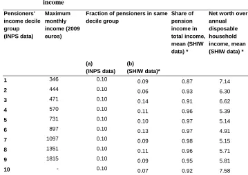
We investigate the representativeness of our sample with respect to pension income and geographical area using the Bank of Italy’s Survey of Households’ Income and Wealth (SHIW) and census data.15 From the first source we find that, in the analyzed years, almost all – more than 98% – males aged 65+ received pension benefits. Table 1 reports detailed information on pensioners’ sources of income for males aged 65+ over the period 1979-2001. The second column reports the maximum income within each income decile that is based on pensioners’ income from the INPS dataset. The third column shows the fraction of pensioners belonging to each INPS-pensioner’ income decile. By definition, these shares are equal to 0.10 when computed in the INPS data (see column “(a) (INPS data)”). Pensioners’ income distribution for the whole population (see “(b) (SHIW data)”) comprises both INPS and non-INPS pensions. This last distribution also includes civil servants and private pensions.16 The reported figures highlight that the INPS data provide a good representation of pension incomes at most deciles.

The fourth column of Table 1 shows the share of pension income in total income (average values). Pension income represents more than 90% of pensioners’ total income with the only exception being individuals in the bottom decile. For this latter group, additional relevant sources of income (values not reported) are both capital income (3%, cf. with 1% for individuals in the third decile and with less than 1% for median individuals) and business or self-employment income (9%, cf. with 5% for individuals in the second decile and 2% for median individuals). This suggests that pension income may be a relatively poor proxy of SES for individuals in the bottom income decile. This suggestion is supported by what is reported in the last column of Table 1, i.e. the

15_{The SHIW data is a survey representative of the entire population of Italy and has been conducted annually}

or biannually since 1977.

16_{To our knowledge, there are no official statistics for the 1980s and the 1990s of pensioners’ income}

(11)

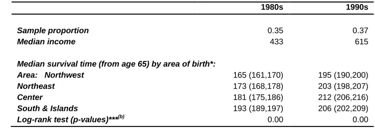
ratio of a household’s net worth (i.e. real and financial wealth minus financial liabilities) over the household’s annual disposable income. This ratio ranges from about 5 to 6.6 for individuals in the second up to and including the ninth deciles, and is over 7 for individuals at the two extremes of the income distribution. Although one can expect this ratio to be higher for individuals in the top decile than for those in the other deciles, the reported value of 7.6 seems rather high and is much higher than the corresponding values for the deciles that are nearest (cf. with 5.8 and 5.7 for individuals in the 9th and 8th deciles respectively). This suggests that for the richest income earners, similar to what we concluded for individuals in the bottom decile, pension income may be a poor proxy of their SES. We will return to some specific issues concerning top income earners in the discussion section. The geographical distribution of the final sample (Northwest: 23.9%, Northeast: 22.2%, Center: 17.6%, South & Islands: 36.4%, see Table 2) matches quite closely that of the corresponding population in the 1991 Census (Northwest: 20.3%, Northeast: 21.5%, Center: 19.1%, South & Islands: 39.1%; ISTAT 2013b).

2.2 Statistical analysis

The analysis is performed on monthly data, from January 1979 to December 2001. We split the whole period into two sub-periods of similar length—January 1979–December 1990 (the “1980s,” follow-up 144 months) and January 1991–December 2001 (the “1990s,” follow-up 132 months).

A preliminary analysis of the association between lifetime income and survival uses Kaplan-Meier survival estimates by income quintiles and areas of birth for the two periods.

(12)

Table 1: Representativeness of the INPS sample with respect to pensioners’ income Pensioners’ income decile group (INPS data) Maximum monthly income (2009 euros)

Fraction of pensioners in same decile group Share of pension income in total income, mean (SHIW data) *

Net worth over annual disposable household income, mean (SHIW data) *

(a) (INPS data)

(b)

(SHIW data)*

1 346 0.10 _0.09 _0.87 _7.14

2 444 0.10 _0.06 _0.93 _6.30

3 471 0.10 _0.14 _0.91 _6.62

4 570 0.10 _0.11 _0.96 _5.39

5 731 0.10 0.10 0.97 5.14

6 897 0.10 _0.13 _0.97 _4.91

7 1097 0.10 _0.09 _0.98 _5.15

8 1351 0.10 _0.11 _0.96 _5.71

9 1815 0.10 _0.09 _0.95 _5.81

10 - 0.10 0.07 0.92 7.58

Note: Males aged 65+, pensions paid in years 1979-2001; *various cross-sections

As discussed in the introduction, we follow Dowd et al. (2011) and Molinari et al. (2001) and implement non-standard free knots spline specifications to model the income–mortality gradient, i.e. a Cox model where the positions and number of the knots in the spline function is determined by the data. As in the standard Cox model, parameter estimates—including the knots parameters—are obtained by maximum likelihood. While being very parsimonious, free knots spline Cox models typically perform better than standard Cox spline (and similar) models in terms of goodness-of-fit (see Molinari et al. 2001) and, in addition, they yield standard errors for the knots.

(13)

we opted for models with a lower number of knots, and the same number of knots for the two periods. Based on these statistical tests we selected a free knot spline Cox model with two knots. Please see Appendix B for further details.17

We use a Hausman test for testing the (joint) hypotheses of equal slope parameters over time. Here we take into account dependence across samples as right-censored individuals in the 1980s sample also belong to the 1990s sample. The variance of the difference between the two parameters vectors was obtained by paired bootstrapping (Cameron and Trivedi 2005).

3. Results

3.1 Empirical findings

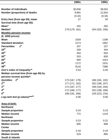
Table 2 shows that 9,991 of the 30,830 males that were alive on the 1st of January 1979 died during the years 1979-1990 (“1980s”), and 12,916 of the 39,054 males that were alive on the 1st of January 1991 died over the years 1991-2001 (“1990s”). Median remaining survival time from age 65 (median survival time henceforth) increased from 179 months (14.9 years) in the 1980s to 204 months (17 years) in the 1990s and the corresponding confidence intervals do not overlap.18 Average monthly pension income was higher in the 1990s than in the 1980s; this mainly reflects economic growth. In addition, there was a moderate reduction in pension income inequality between the 1980s and the 1990s. In the 1980s, median survival time is equal to 173 months for the first income quintile, and to 198 months for the fifth, revealing an absolute difference in median survival time of 25 months between the poorest and the richest group and a relative difference of 14%. In the same period, the median survival time is almost invariant between the first and the fourth income quintiles. Based on a log-rank test we reject the hypothesis of equality of survivor functions across income quintiles (the p-value is equal to 0). In the 1990s, median survival is equal to 186 months for the first income quintile and 229 months for the fifth income quintile: an absolute difference of 43 months and a relative difference of 23%. Unlike in the 1980s, in the 1990s individuals in the second income quintile had a significantly higher median survival time than those in the first income quintile. As for the 1980s, there was no difference in survival between the second and the fourth income quintile. Confidence intervals for

17_{Similar to what we did, Montez et al. (2012) compare several functional forms of the association between}

SES (education) and the risk of death.

18_{Mean survival times are somewhat higher than life expectancies at age 65 reported in HMD (2013): 191}

(14)

median survival time for the same income quintiles in the 1980s and the 1990s do not overlap.

Figure 1 reports Kaplan-Meier survival curves for individuals in the first and fifth income quintile and (population) survival curves from the Human Mortality Database (HMD 2013) by decade. As mentioned in the previous section, the two samples are dependent as survivors from the left panel of the figure are also present in the right panel and we take this into account when testing for differences in the slope parameters between these two periods. In line with the results reported in Table 2 in terms of median survival time, the figure shows that mortality rates are significantly lower for individuals in the top income quintile than for those in the bottom quintile. It also highlights that, for both decades, the population-based survival curve from HMD lies very close to our survival curve for the bottom income quintile. This suggests that HMD mortality rates are somewhat higher than in our data. It should, however, be noted that the two populations are different, since we consider ex-workers, whereas HMD includes the whole population. Wolfson et al. (1993) report a similar degree of underestimation of mortality rates when comparing their data from a Canadian pension plan with census data.

(15)

Table 2: Descriptive statistics

1980s 1990s

Number of individuals 30,830 39,054

Number (proportion) of deaths 9,991

(0.32)

12,916 (0.33)

Entry time (from age 65), mean 27 54

Survival time (from age 65):

Mean* 191 202

Median* 179 (176, 181) 204 (202, 206)

Monthly pension income: (€, 2009 prices):

Mean 1029 1198

Standard deviation 2173 1952

Percentiles: 1st ₂₀₇ ₂₂₇

20th 328 444

40th 454 653

50th 533 828

60th 694 1013

80th ₁₁₇₂ ₁₅₃₁

99th 9116 7386

Gini’s index of inequality** 0.53 0.45

Median survival time (from age 65) by pension income quintile*:

Quintiles: 1th 173 (167, 179) 186 (181, 192)

2nd 177 (171, 182) 202 (196, 207)

3rd 172 (167, 177) 199 (194, 204)

4th 172 (168, 177) 202 (196, 208)

5th _{198 (191, 206)} _{229 (223, 234)}

Log-rank test (p-values)***(a) 0.00 0.00

Area of birth: Northwest

Sample proportion 0.24 0.23

Median income 772 1119

Northeast

Center

(16)

Table 2: (Continued)

1980s 1990s

Median survival time (from age 65) by area of birth*:

Area: Northwest 165 (161,170) 195 (190,200)

Northeast 173 (168,178) 203 (198,207)

Center 181 (175,186) 212 (206,216)

South & Islands 193 (189,197) 206 (202,209)

Log-rank test (p-values)***(b) 0.00 0.00

Note: Entry time and survival estimates are given in months and correspond to the starting age equal to 65 years (780 months). * Kaplan-Meier survival estimates; 95% confidence interval in brackets; mean survival time computed on exponentially extended survivor functions

** Ranges between one (maximum inequality) and zero (no inequality)

*** The null-hypothesis is equality of survival functions across (a) pension income quintiles and (b) areas of birth.

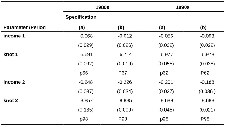
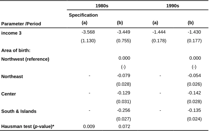
Table 3 reports the parameter estimates for the model outlined in Section 2. The table presents estimates for two empirical specifications: specification (a) only includes pension income as explanatory variable; specification (b) includes areas of birth as additional covariates. Figures 2 and 3 present predictions based on these estimates.

(17)

Figure 1: Kaplan-Meier survival estimates by income quintile

(q=1 corresponds to the 1st quintile, q=5 to the 5th quintile) and (population) survival curves from the Human Mortality Database (HMD 2013) by decade (the 1980s and 1990s)

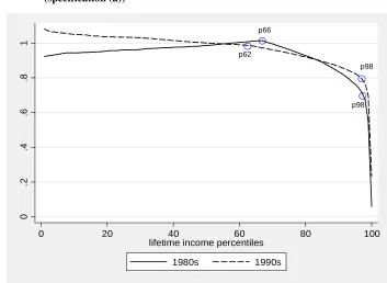
Using specification (a), the results for the 1990s show that the positions of the two knots in the income–mortality gradient are by and large the same as for the 1980s. However, the income 1 slope parameter has changed considerably over time. For individuals with income below the 62nd income percentile (p62), the estimated association is negative in the 1990s and implies that a 1% higher income is associated with a 0.06% lower mortality risk. The same unitary change is associated with a reduction in top earners’ risk of death in the 1990s by 1.4% (cf. with 3.6% in the 1980s; this difference is, however, not statistically different from zero). There are few changes between the 1980s and the 1990s for individuals with lifetime income between the 62nd/66th and the 98th percentiles (cf. income 2 parameters). The p-value corresponding to a Hausman test of the null-hypothesis of an equal income-mortality gradient over

0

.25

.5

.75

1

0 100 200 300

analysis time

95% CI

q = 1 q = 5

HMD 1980-89

1980s

0

.25

.5

.75

1

0 100 200 300 400

analysis time

95% CI

q = 1 q = 5

HMD 1990-99

(18)

time is equal to 0.009. This evidence is in favor of an overall changing income– mortality gradient over time.

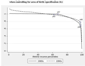
The results when areas of birth are included (specification (b)) show a negative estimate for the income 1 coefficient that is not statistically different from zero for the 1980s. The estimate for the income 1 coefficient is also somewhat higher for the 1990s (compared to specification (a)). Our estimates confirm that males living (and working) in the industrialized Northwest of the country have higher mortality compared to those living in other parts of Italy. Meanwhile, males in the Northwest also have higher median income (Table 2, cf. with median income in South & Islands). Conditional on living in a particular area, the effect of individual income on mortality is thus strengthened. We speculate that this effect occurs only for males with an income below the 62nd/66th percentile (knot 1), as it especially affects manual workers.

Results for specification (b) set forth in Table 3 also show that once controlled for area of birth, the estimate of the income 1 parameter does not change over time in a significant way (cf. with specification (a)). The Hausman test suggests that— conditioning on living in a given area of the country—the association between income and mortality remained unchanged between the 1980s to the 1990s (p-value 0.07). Regional differences in mortality—higher mortality in the Northwest and particularly in the 1980s—and income thus explain a large part of the time evolution of the income– mortality association reported in Table 3, specification (a).

Table 3: Two free knots spline Cox models: parameter estimates

Parameter /Period

1980s 1990s

Specification

(a) (b) (a) (b)

income 1 0.068 -0.012 -0.056 -0.093

(0.029) (0.026) (0.022) (0.022)

knot 1 6.691 6.714 6.977 6.978

(0.092) (0.019) (0.055) (0.038)

p66 P67 p62 P62

income 2 -0.248 -0.226 -0.201 -0.188

(0.037) (0.034) (0.037) (0.036 )

knot 2 8.857 8.835 8.689 8.688

(0.135) (0.009) (0.045) (0.021)

(19)

Table 3: (Continued)

1980s 1990s

Specification

(a) (b) (a) (b)

income 3 -3.568 -3.449 -1.444 -1.430

(1.130) (0.755) (0.178) (0.177)

Area of birth:

Northwest (reference) 0.000 0.000

(-) (-)

Northeast - -0.079 - -0.054

(0.028) (0.026)

Center - -0.129 - -0.142

(0.031) (0.028)

South & Islands - -0.256 - -0.135

(0.027) (0.024)

Hausman test (p-value)* 0.009 0.072

Notes: Males, models by decade. Specification (a) excludes area of birth dummy variables and specification (b) includes area of birth

dummy variables. The spline function with endogenously determined knots; income x is the percentage change in the hazard of death associated with a 1% increase in the lifetime (pension) income for levels of log-income in the interval [knot x-1, knot x];

knot x is the estimated knot of the log-income spline function; in italics we report the position of the estimated knot in the

sample-specific log-income distribution; standard error in parenthesis; * χ2

-test on the equality of the income (slope) parameters in the 1980s versus the 1990s samples.

3.2 Robustness checks

(20)

results from our models using the free knots spline Cox specifications. Our results turned out to be robust to all these modifications.

Figure 2: Average predicted hazard ratios by income percentile and decade (specification (a))

Notes: Two free knots spline model, the circles indicate the positions of the estimated knots: p62 is the 62nd percentile, p66 is

the 66th

percentile and p98 is the 98th

percentile of the period-specific income distribution.

In addition, we have gathered reassuring evidence that the potential measurement error in pension income is unlikely to influence our findings. This issue may arise for private sector employees who contributed to other pension schemes managed by non-INPS institutions during their working career. For example, if an individual has worked both in the private and in the public sector for sufficiently long periods to accrue pension rights in both respective funds, we would underestimate his total pension

p66

p98 p62

p98

0

.2

.4

.6

.8

1

0 20 40 60 80 100

lifetime income percentiles

(21)

income.19 To obtain insight into this issue we have used information from a different pension file for the period 1995–2000 (drawn from the Casellario dei Pensionati archive) on non-INPS pensions—i.e., public sector pensions and minor pension funds managed by large firms. We find that only a very small percentage of males (1.7%) receive pensions from both INPS and non-INPS institutions.

Figure 3: Average predicted hazard ratios by income percentile and decade when controlling for area of birth (specification (b))

Notes: Two free knots spline model, the circles indicate the positions of the estimated knots: p62 is the 62nd

percentile, p67 is the 67th

19_{To control for this, Gaudecker and Scholz (2007) use information on the number of years of}

pension-relevant insurance periods (and the type of health insurance coverage) and estimate mortality rates for different subsamples. We do not have this information in our data.

p62 p67

p98 p98

0

.2

.4

.6

.8

1

0 20 40 60 80 100

(22)

In this study we proxy area of living by means of area of birth. This is a good proxy for the cohorts we analyze (1901-36), as they did not migrate within Italy that much. Indeed, internal migrations (rural to urban and South to North) were very pronounced in the first and last years of the 1960s (Bonifazi and Heinz 2000) and especially involved young males (the average age at migration was 23; see Dan and Fornasin 2013). We find a confirmation of this phenomenon from the Bank of Italy's survey SHIW (used in Table 1): From this data, it appears that less than 3% of males born in 1901-36 alive at age 65 had migrated from the underdeveloped South & Islands to the industrialized Northwest.

Furthermore, the main empirical results are unaffected when controlling for other covariates such as year of birth, retirement age, or receipt of a disability pension. These additional results are available from the authors upon request.

Finally, in our analysis we model mortality risk from age 65 onwards. Individuals may, however, retire earlier but this may be related to health (hence to mortality risk). We therefore did not take the time before age 65 into account. Nevertheless, analyzing the mortality risk from the age when individuals in our sample received a pension for the first time (and this could be before age 65) did not affect our main findings in terms of both time evolution and shape of the income-mortality gradient.

3.3 Discussion

As noted in the introduction, the existing evidence on the shape of the lifetime income– old age mortality gradient is scarce and mixed. Some authors find a concave relationship between these two variables and others do not. Leombruni et al. (2010) find for Italy that only retirees in the highest quintile of the income distribution benefit from significantly lower mortality risk in comparison to the rest of the retired population. Our results are in line with those of Leombruni et al. (2010) and show that, across most of the income distribution, the income-old age mortality gradient is weak in Italy. One possible explanation of these findings relates to confounding factors. Data on educational attainment and working career characteristics, which we do not have, could certainly yield further explanations. Shkolnikov et al. (2007), however, show for Germany that adjustment for other SES factors leads to a marginal weakening of the income-mortality gradient.

(23)

earnings for individuals in the bottom and probably the top decile of the pension income distribution. This measurement error problem is well known in the literature. For instance, and in line with our study, Wolfson et al. (1993) point out the existence of unobserved earnings especially at the lower end of the income distribution. As described in the introduction, Shkolnikov et al. (2007) and von Gaudecker and Scholz (2007) attribute their evidence of a counterintuitive J-shaped relation between life expectancy at age 65 and lifetime earnings in Germany to unobserved earnings. They report a positive association between these two variables across the whole pension income distribution for Eastern Germany where, for institutional reasons, such a measurement error issue is much less relevant. Von Gaudecker and Scholz (2007) also point out that for the whole country, such a positive association is almost linear if one focuses on the central part of the pension income distribution (of longer-insured workers), where the measurement error problem is reduced. Moreover, it is worth pointing out that the measurement error problem in earnings may be more severe in Italy – and more generally in southern European countries – than in other countries due to closer family ties (Alesina et al. 2010) and informal earnings (Schneider and Enste 2000).

We should interpret with caution the results for top earners whose estimated income– mortality gradient is particularly steep. From a statistical point of view, the estimates of the slope parameters above the highest positioned knot are relatively imprecise (relatively high standard errors, especially in the 1980s). Moreover, for top earners observed pension income can be a particularly poor proxy of lifetime income for the following reasons. First, top earners may have substantial income from financial assets and housing wealth. Alvaredo et al. (2012) report that in Italy, in 1990, 24% of incomes of the top-1% earners were either capital income or rents, while wages and pensions represented only 37%; corresponding figures for the top 10–5% were 7% and 83%, respectively. Second, top earners are typically executives and highly qualified workers who are often enrolled in special pension schemes. Their actual pension income can be higher than what is observed due to lump-sum compensation or additional annuities (unobserved in this data) that are often granted by employers to lay off these high-cost workers or as a final premium for their working careers. Third, the work-package agreement for top earners was extremely generous (often including private health insurance coverage and various in-kind benefits) and, therefore, their SES was higher than implied by their income.

(24)

The delay of the smoking “epidemic” in southern Europe may explain why old age mortality inequalities by SES have been smaller in Italy than in other countries.20 In the introduction, we reported the existence of a north-south gradient in smoking prevalence by SES among older European males around 1990 (Cavelaars et al. 2000). A delay in the smoking “epidemic” may also explain why mortality inequalities by SES have not widened throughout the analyzed period. Federico et al. (2004) report that the observed decline in smoking prevalence among Italian males aged 50+ in the period 1980-2000 has been homogenous across socioeconomic groups.21 This is consistent with the findings of Cavelaars et al. (2000) and Huisman et al. (2005) – referring to early and late 1990s, respectively, both works find a similar level of educational differences in smoking prevalence among Italian older males. In terms of north-south gradient among older European males, however, these works report different results. Huisman et al. (2005) do not find any evidence of the gradient found 10 years earlier by Cavelaars et al. (2000). This 10-years change in the north-south gradient is fully consistent with the smoking “epidemic” diffusion model (see discussion in Huisman et al. 2005). Finally, studies from the US also find a trend in the smoking pattern similar to the one found for northern European countries: Among Americans aged 65+, the prevalence of current smoking over the period 1970-1994 declined only for individuals with more than 11 years of education (Husten et al. 1997).

In this study, we cannot analyze behavioral changes, nor do we have causes of death information to explore the causes of any time change in the income–old age mortality gradient in any depth. Nevertheless, in this paper, we complete an important first step and show that it is necessary to account for regional differences when examining changes in the income–mortality gradient in Italy, and that after doing so, that the income-old age mortality gradient turns out to be rather stable over time.

4. Conclusions

This is the first study on the time trend of the association between lifetime income and old age mortality risk in Italy. In addition, this study provides further empirical evidence on the shape of the income–old age mortality association for Italy. The analysis makes use of a sample of ex-private sector workers aged 65 and over from a

20_{Federico et al. (2013) provide empirical evidence in favor of this hypothesis. They quantify the contribution}

of smoking to the SES-mortality gradient for the Italian population aged 30-74, i.e. not specifically for the elderly.

21_{Gorini et al. (2013) give updated evidence on trends of social differences in smoking habits in Italy. This}

(25)

newly available pension database drawn from an administrative archive held by the primary Italian social security institution.

The association between lifetime income and old age mortality risk in Italy is negative but weak across most of the income distribution. After having controlled for regional differences, we see that the income-old age mortality gradient is rather stable over time. This evidence is consistent with a declining trend in behavioural risk factors (e.g. smoking) among elderly people which is fairly homogeneous across different socioeconomic statuses.

5. Acknowledgments

(26)

References

Alesina, A.F., Algan, Y., Cahuc, P., and Giuliano, P. (2010). Family Values and the Regulation of Labor. Cambridge, MA: National Bureau of Economic Research, Inc. (NBER Working Papers n. 15747).

Alvaredo, F., Atkinson, A.B., Piketty, T., and Saez, E. (2012). The World Top Incomes Database [electronic resource]. Paris: Paris School of Economics. http://topincomes.g-mond.parisschoolofeconomics.eu/.

Antonovsky, A. (1967). Social class, life expectancy, and overall mortality. The Milbank Memorial Fund Quarterly 45(2): 31–73. doi:10.2307/3348839.

Belloni, M. and Alessie, R. (2009). The importance of financial incentives on retirement choices: new evidence for Italy. Labour Economics 16(5): 578–588. doi:10.1016/j.labeco.2009.01.008.

Belloni, M. and Maccheroni, C. (2013). Actuarial Neutrality when Longevity Increases: An Application to the Italian Pension System. The Geneva Papers on Risk and Insurance - Issues and Practice 38(4): 638–674. doi:10.1057/gpp.2013.27.

Bonifazi, C. and Heins, F. (2000). Long-term trends of internal migration in Italy. International Journal of Population Geography 6(2): 111–131. doi:10.1002/(SICI)1099-1220(200003/04)6:2<111::AID-IJPG172>3.3.CO;2-C.

Bos, V., Kunst, A.E., and Mackenbach, J.P. (2002). Socioeconomic inequalities in mortality in the Netherlands: analyses on the basis of information at the neighborhood level. TSG Tijdschrift voor Gezondheidswetenschappen 80: 158–165.

Bratti, M (2003). Labour force participation and marital fertility of Italian women: The role of education. Journal of Population Economics 16(3): 525–554. doi:10.1007/s00148-003-0142-5.

Brugiavini, A. and Galasso, V. (2004). The Social Security Reform Process in Italy: Where Do We Stand? Journal of Pension Economics and Finance 3(2): 165–195. doi:10.1017/S1474747204001568.

(27)

Cameron, C. and Trivedi, P.K. (2005). Microeconometrics: Methods and Applications. Cambridge, UK: Cambridge University Press. doi:10.1017/ CBO9780511811241.

Cavelaars A.E., Kunst, A.E., Geurts, J.J., Crialesi, R., Grötvedt, L., Helmert, U., Lahelma, E., Lundberg, O., Matheson, J., Mielck, A., Rasmussen, N.K., Regidor, E., do Rosário-Giraldes, M., Spuhler, T., and Mackenbach, J.P. (2000). Educational differences in smoking: international comparison. BMJ 320(7242): 1102–1107. doi:10.1136/bmj.320.7242.1102.

Centers for Disease Control and Prevention (CDC) (2012). Health Equity [electronic resource]. Atlanta: National Center for Chronic Disease Prevention and Health Promotion. www.cdc.gov/chronicdisease/healthequity/index.htm.

Cesaroni, G., Agabiti, N., Forastiere, F., Ancona, C., and Perucci, C.A. (2006) Socioeconomic differentials in premature mortality in Rome: changes from 1990 to 2001. BMC Public Health 6(1): 270. doi:10.1186/1471-2458-6-270.

Christia, J.P. (2009). Rising mortality and life expectancy differentials by lifetime earnings in the United States. Journal of Health Economics 28(5): 984–995. doi:10.1016/j.jhealeco.2009.06.003.

Commission of the European Communities (COM) (2007). White paper: Together for Health: a Strategic Approach for the EU 2008-2013, COM 630. Brussels: 23.10.2007.

Commission of the European Communities, Communication from the Commission to the European Parliament, the Council, the European Economic and Social Committee and the Committee of the Regions (COM) (2009). Solidarity in Health: Reducing Health Inequalities in the EU, COM 567. Brussels: 20.10.2009.

Commission on Social Determinants of Health (CSDH) (2008). Closing the gap in a generation: health equity through action on the social determinants of health. Final Report of the Commission on Social Determinants of Health. Geneva: World Health Organization.

Cox, D.R. (1972). Regression models and life-tables. Journal of the Royal Statistical Society. Series B (Methodological) 34(2): 187–220.

(28)

Dan, N., and Fornasin, A. (2013). Una indagine CATI per lo studio della mobilità interna in Italia in un’ottica longitudinale. Udine: Dept. of Economics and Statistics of University of Udine. (Working paper n. 4/2013).

Dowd, J.B., Albright, J., Raghunathan, T.E., Schoeni, R.F., LeClere, F., and Kaplan, G.A. (2011). Deeper and wider: income and mortality in the USA over three decades. International Journal of Epidemiology 40(1): 183–188. doi:10.1093/ ije/dyq189.

Duleep, H.O. (1986). Measuring the effect of income on adult mortality using longitudinal administrative record data. The Journal of Human Resources 21(2): 238–251. doi:10.2307/145800.

Federico, B., Kunst, A.E., Vannoni, F., Damiani, G., and Costa G., (2004). Trends in educational inequa lities in smoking in northern, mid and southern Italy, 1980-2000. Preventive Medicine 39(5): 919–926. doi:10.1016/j.ypmed.2004.03.029. Federico, B., Mackenbach, J.P., Eikemo, T.A., Sebastiani, G., Marinacci, C., Costa, G.,

and Kunst, A.E. (2013). Educational inequalities in mortality in northern, mid and southern Italy and the contribution of smoking. Journal of Epidemiology and Community Health 67(7): 603–609. doi:10.1136/jech-2012-201716.

Felice, E. (2010). Regional development: reviewing the Italian mosaic. Journal of Modern Italian Studies 15(1): 64–80. doi:10.1080/13545710903465556.

Ferrie, J.E., Shipley, M.J., Marmot, M.G., Stansfeld, S.A., and Smith, G.D. (1998). An Uncertain Future: The Health Effects of Threats to Employment Security in White-Collar Men and Women. American Journal of Public Health 88(7): 1030–1036. doi:10.2105/AJPH.88.7.1030.

Galobardes, B., Shaw, M., Lawlor, D.A., Lynch, J.W., and Davey Smith, G. (2006). Indicators of socioeconomic position (Part 1). Journal of Epidemiology and Community Health 60(1): 7–12. doi:10.1136/jech.2004.023531.

Gorini, G., Carreras, G., Allara, E., and Faggiano, F. (2103). Decennial trends of social differences in smoking habits in Italy: a 30-year update. Cancer Causes Control 24(7): 1385–1391. doi:10.1007/s10552-013-0218-9.

(29)

Huisman, M., Kunst A.E., and Mackenbach, J.P. (2005). Educational inequalities in smoking among men and women aged 16 years and older in 11 European countries. Tobacco Control 14(2): 106–113. doi:10.1136/tc.2004.008573.

Huisman, M., Kunst, A.E., Andersen, O., Bopp, M., Borgan, J.K., Borrell, C., Costa, G., Deboosere, P., Desplanques, G., Donkin, A., Gadeyne, S., Minder, C., Regidor, E., Spadea, T., Valkonen, T., and Mackenbach, J.P. (2004). Socioeconomic inequalities in mortality among elderly people in 11 European populations. Journal of Epidemiology and Community Health 58(6): 468–475. doi:10.1136/jech.2003.010496.

Human Mortality Database (HMD) (2013). The Human Mortality Database [electronic resource]. Berkeley and Rostock: University of California, Berkeley, and Max Planck Institute for Demographic Research. www.mortality.org.

Husten, C.G., Shelton, D.M., Chrismon, J.H., Lin, Y.C., Mowery, P., and Powell, F.A. (1997). Cigarette smoking and smoking cessation among older adults: United States, 1965–94. Tobacco Control 6(3): 175-180. doi:10.1136/tc.6.3.175.

ISTAT (2012). Tavole di Mortalità della popolazione italiana per provincia e regione di residenza. Rome: ISTAT. http://demo.istat.it.

ISTAT (2013). Serie storiche: L’archivio della Statistica Italiana [electronic resource]. Rome: ISTAT. http://seriestoriche.istat.it/.

ISTAT (2013b). Censimento popolazione e abitazioni 1991 – campione all’1%. Rome: ISTAT. http://www.istat.it/it/archivio/3758.

Kalwij, A., Alessie, R., and Knoef, M. (2013). The association between individual income and remaining life expectancy at the age of 65 in the Netherlands. Demography 50(1): 181–206. doi:10.1007/s13524-012-0139-3.

Kibele, E.U.B., Jasilionis, D., and Shkolnikov, V.M. (2013). Widening socioeconomic differences in mortality among men aged 65 years and older in Germany. Journal of Epidemiology and Community Health 67(5): 453–457. doi:10.1136/ jech-2012-201761.

(30)

Kunst, A.E., Bos, V., Andersen, O., Cardano, M., Costa, G., Harding, S., Hemström, Ö., Layte, R., Regidor, E., Reid, A., Santana, P., Valkonen, T., and Mackenbach, J.P. (2004). Monitoring of trends in socioeconomic inequalities in mortality: Experiences from a European project. Demographic Research Special Collection 2(9): 229–254. doi:10.4054/DemRes.2004.S2.9.

Leombruni, R., Richiardi, M., Demaria, M., and Costa, G. (2010). Aspettative di vita, lavori usuranti ed equità del sistema previdenziale. Prime evidenze dal Work Histories Italian Panel. Epidemiologia e Prevenzione 34(4): 150–158.

Lindstrom, M. (2008). Social capital and health-related behaviors. In: Kawachi, I., Subramanian, S.V., and Kim, D. (eds). Social capital and health. Boston, MA: Springer: 215–238. doi:10.1007/978-0-387-71311-3_10.

Mackenbach, J.P., Bos, V., Andersen, O., Cardano, M., Costa, G., Harding, S., Reid, A., Hemström, Ö., Valkonen, T., and Kunst, A.E. (2003). Widening socioeconomic inequalities in mortality in six Western European countries. International Journal of Epidemiology 32(5): 830–837. doi:10.1093/ije/dyg209.

Mackenbach, J.P., Stirbu, I., Roskam, A.J.R., Schaap M.M., Menvielle, G., Leinsalu, M., and Kunst, A.E. (2008). Socioeconomic inequalities in health in 22 European countries. The New England Journal of Medicine 358(23): 2468–2481. doi:10.1056/NEJMsa0707519.

Marinacci, C., Grippo, F., Pappagallo, M., Sebastiani, G., Demaria, M., Vittori, P., Caranci, N., and Costa, G. (2013). Social inequalities in total and cause-specific mortality of a sample of the Italian population, from 1999 to 2007. The European Journal of Public Health 23(4): 582–587. doi:10.1093/eurpub/cks184.

Marinacci, C., Spadea, T., Biggeri, A., Demaria, M., Caiazzo, A., and Costa, G. (2004). The role of individual and contextual socioeconomic circumstances on mortality: analysis of time variations in a city of north west Italy. Journal of Epidemiology and Community Health 58(3): 199–207. doi:10.1136/jech.2003.014928.

Materia, E., Spadea, T., Rossi, L., Cesaroni, G., Areà, M., and Perucci, C.A. (1999). Health care inequalities: hospitalization and socioeconomic position in Rome. Epidemiologia e Prevenzione 23(3):197–206.

(31)

Molinari, N., Daurès, J.P., and Durand, J.F. (2001). Regression splines for threshold selection in survival data analysis. Statistics in Medicine 20(2): 237–247. doi:10.1002/1097-0258(20010130)20:2<237::AID-SIM654>3.0.CO;2-I.

Montez, J.K., Hummer, R.A., and Hayward, M.D. (2012). Educational Attainment and Adult Mortality in the United States: A Systematic Analysis of Functional Form. Demography 49(1): 315–336. doi:10.1007/s13524-011-0082-8.

Peracchi, F. (2008). Height and Economic Development in Italy, 1730-1980. American Economic Review: 98(2): 475–481. doi:10.1257/aer.98.2.475.

Prättala, R., Hakala, S., Roskam, A.J., Roos, E., Helmert, U., Klumbiene, J., Van Oyen, H., Regidor, E., and Kunst, A.E. (2009). Association between educational level and vegetable use in nine European countries. Public Health Nutrition 12(1): 2174–2182. doi:10.1017/S136898000900559X.

Schneider, F. and Enste, D.H. (2000). Shadow Economies: Size, Causes, and Consequences. Journal of Economic Literature 38(1): 77–114. doi:10.1257/ jel.38.1.77.

Shkolnikov, V.M., Scholz, R., Jdanov, D.A., Stegmann, M., and von Gaudecker, H.M. (2007). Length of life and pensions of five million retired German men. European Journal of Public Health 18(3): 264–269. doi:10.1093/eurpub/ ckm102.

Sullivan, D. and von Wachter, T. (2009). Average earnings and long-term mortality: evidence from administrative data. American Economic Review: Papers & Proceedings 99(2): 133–138. doi:10.1257/aer.99.2.133.

van den Berg, G., Lindeboom, M., and Portrait, F. (2006). Conjugal Bereavement Effects on Health and Mortality at Advanced Ages. Bonn: Institute for the Study of Labor. (IZA discussion paper n. 2358).

Vittorio, D. and Paolo, M.. (2007). Il prodotto delle regioni e il divario Nord-Sud in Italia (1861–2004). Rivista di Politica Economica 97(2):267-316.

von Gaudecker, H.M. and Scholz, R.D. (2007) Differential mortality by lifetime earnings in Germany. Demographic Research 17(4): 83–108. doi:10.4054/ DemRes.2007.17.4.

(32)

Wilmoth, J.R. and Dennis, M. (2007). Social differences in older adult mortality in the United States: questions, data, methods, and results. In: Robine, J.M., Crimmins, E.M., Horiuchi, S., and Zeng, Y. (eds.). Human Longevity, Individual Life Duration, and the Growth of the Oldest-Old Population, Dordrecht: Springer: 297–332. doi:10.1007/978-1-4020-4848-7_14.

(33)

Appendix A: Results for females

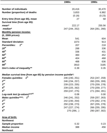
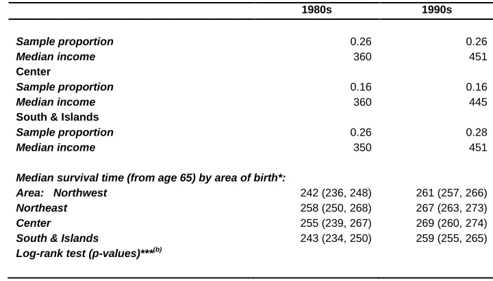
In this appendix we report the main results for females to which all caveats discussed in Section 2.1 apply. Table A1 reports summary statistics for the female sample. The table shows that females’ income distributions are much more compressed than males’ – in particular at their upper end (cf. income percentiles in Tables 1 and A1). Females’ median survival times by males’ income quintile highlight that the differences between top and bottom income groups (1980s: absolute difference 29 months, relative difference 12%; 1990s: absolute difference 31 months, relative difference 12%) are in line with those reported for males (cf. with Table 1). This suggests that possible gender differences in the income-mortality gradient can be the result of differences in the income distributions.

(34)

Table A1: Descriptive statistics: females

1980s 1990s

Number of individuals 20,416 30,470

Number (proportion) of deaths 3,653

(0.18)

6,982 (0.23)

Entry time (from age 65), mean 27 58

Survival time (from age 65):

mean* 222.17 255.56

median* 247 (244, 252) 264 (261, 266)

Monthly pension income: (€, 2009 prices):

Mean 541 604

Standard deviation 1073 913

Percentiles: 1st 207 218

20th 288 336

40th ₃₃₆ ₄₃₁

50th 360 452

60th ₄₀₄ ₄₆₈

80th 488 636

99th 3910 3185

Gini’s index of inequality** 0.39 0.35

Median survival time (from age 65) by pension income quintile*:

Females quintiles: 1th 246 (240, 251) 253 (247, 259)

2nd _{246 (234, 257)} _{260 (255, 269)}

3rd 239 (223, 255) 270 (259, 278)

4th _{239 (225, 262)} _{270 (259, 277)}

5th 259 (247, 275) 271 (264, 281)

Log-rank test (p-values)***(a) 0.08 0.00

Males quintiles****: 1th 246 (241, 252) 259 (257, 263)

2nd 242 (230, 254) 270 (262, 274)

3rd _{250 (238, 273)} _{267 (255, 278)}

4th 247 (227, 274) 266 (255, 295)

5th _{275 (266, .)} _{290 (267, 302)}

Area of birth: Northwest

(35)

Table A1: (Continued)

1980s 1990s

Center

South & Islands

Median survival time (from age 65) by area of birth*:

Area: Northwest 242 (236, 248) 261 (257, 266)

Northeast 258 (250, 268) 267 (263, 273)

Center 255 (239, 267) 269 (260, 274)

South & Islands 243 (234, 250) 259 (255, 265)

Log-rank test (p-values)***(b)

Note: Entry time and survival estimates are given in months and correspond to the starting age equal to 65 years (780 months). * Kaplan-Meier survival estimates; 95% confidence interval in brackets; mean survival time restricted to longest follow-up ** Ranges between one (maximum inequality) and zero (no inequality)

(36)

Table A2: One free knot spline Cox models: parameter estimates - females

1980s 1990s

Specification

(a) (b) (a) (b)

income 1 -0.063 -0.085 -0.102 -0.116

(0.042) (0.040) (0.027) (0.026)

knot 1 7.757 7.977 8.238 8.668

(0.220) (0.031) (0.063) (0.085)

p97 p98 p99 p99

income 2 -1.867 -2.645 -0.738 -0.944

(0.754) (0.823) (0.202) (0.306)

Area of birth:

Northwest (reference) 0.000 0.000

(-) (-)

Northeast - -0.147 - -0.091

(0.044) (0.031)

Center - -0.136 - -0.105

(0.051) (0.037)

South & Islands - -0.025 - -0.020

(0.044) (0.032)

Hausman test (p-value)* 0.673 0.717

Notes: Females, models by decade. Specification (a) excludes area of birth dummy variables and specification (b) includes area of

birth dummy variables. The spline function with endogenously determined knots; income x is the percentage change in the hazard of death associated with a 1% increase in the lifetime (pension) income for levels of log-income in the interval [knot x-1,

knot x]; knot x is the estimated knot of the log-income spline function. In italics we report the position of the estimated knot in the

sample-specific log-income distribution; standard error in parenthesis. * χ2

(37)

Figure A1: Average predicted hazard ratios for females by income percentile and decade

Notes: One free knot spline model with specification (a), the circles indicate the positions of the estimated knots. P97 is the 97th

p97

p98

.2

.4

.6

.8

1

1.

2

0 20 40 60 80 100

(38)

Figure A2: Average predicted hazard ratios by males’ income percentile: males versus females (top panel: 1980s, bottom panel: 1990s)

Notes: Males: two free knots spline model; Females: one free knot spline model; specification (b)

.2

.4

.6

.8

1

1.

2

0 20 40 60 80 100

males' lifetime income percentiles

Males Females

1980s

0

.2

.4

.6

.8

1

1.

2

0 20 40 60 80 100

males' lifetime income percentile

Males Females

(39)

Appendix B: Testing

Table B1 shows likelihood-based goodness-of-fit measures: AIC, BIC, and an LR-test against the log-linear model. Notice that (i) free knots models with a different number of knots are not nested; (ii) all estimated models are nested in the log-linear model. An alternative test to AIC/BIC is an “indirect” LR-test (Molinari 2001), in which each model is compared with the log-linear model.

Table B1: Model selection

Model: d.f. -2x log(Lik) LR-test* AIC BIC

Males - 1980s

log-linear 1 180988 - 180990 180998

log-linear spline with 5 knots 5 180876 2.73E-23 180886 180928

log-linear spline with 1 free knot 3 180852 2.98E-30 180858 180883

log-linear spline with 2 free knots 5 180821 4.67E-35 180831 180873

Males - 1990s

log-linear 1 229070 - 229072 229081

log-linear spline with 1 free knot 3 228935 5.97E-30 228941 228967

Females - 1980s

log-linear 1 62464 - 62466 62474