0 INTRODUCTION
In recent years, stainless steels have been increasingly utilised in the automotive industry and in the production of domestic appliances because of its excellent strength, good formability and resistance to corrosion. While the use of stainless steel increases mechanical properties of a formed part, there is another merely technological disadvantage. We refer to the so–called springback effect, a phenomenon that is associated with the reversible elastic strain recovery which happens after the removal of the tools and complete unloading of the formed part. Because of the high stress state that is achieved in stainless steels during forming, and because of smaller sheet thickness that is usually required in order to reduce the weight of the produced component, the springback of stainless steels in regard to forming mild steels is even more intense and has been long recognised as a major problem for companies’ development departments. From the point of view of tool design, there is no doubt that a reliable springback prediction, which is based on the corresponding numerical simulation of the forming process, is the key to resolving this problem. In this regard, a considerable amount of work that is specifically related to the proper mathematical modelling of the springback has been already done. Above all, it turns out that the precise experimental observation of the material’s behaviour and the inclusion of its revealed physical relations into a corresponding constitutive model are the most promising way. Models that have been presented up until now mostly deal with the precise modelling of
anisotropy [1], the Bauschinger effect [2], and damage [3]. Recently, we have proposed that, for reliable springback prediction, elastic modulus degradation must also be included in the constitutive modelling; in [4] we studied the effect of coupling the Mori–Tanaka model with isotropic plasticity. However, sheet metals usually exhibit significant plastic anisotropy. This paper is an attempt to build a corresponding physically consistent constitutive model that is capable of taking into account the resulting stiffness degradation during plastic deforming and plastic anisotropy in material.
The topic presented here, which is focused on the anisotropy modelling and experimental verification of the basic assumptions, is in this regard a continuation and an upgrade of our previous research, as reported in [5] and [4]. The work is based on a combined experimental–analytical–numerical approach; with the proven experimental evidence being analytically modelled, the physical adequacy of the built constitutive equations is established by means of a numerical simulation of given experiments. The conceived constitutive model is implemented into a FEM-based program; in our case, ABAQUS/Explicit [6]. In the development stage of the constitutive modelling, the FEM simulations are used purely for the purpose of constructing a constitutive model that is as consistent as possible with the given experimental evidence. In the end, with the developed constitutive model being confirmed in regard to its original experimental framework, it is further numerically validated on a simulation of a series of experimentally performed springback tests.
Advanced Modelling of Sheet Metal Forming
Considering Anisotropy and Young’s Modulus Evolution
Starman, B. – Vrh, M. – Halilovič, M. – Štok, B. Bojan Starman – Marko Vrh – Mirko Halilovič – Boris Štok*
University of Ljubljana, Faculty of Mechanical Engineering, Slovenia
The paper focuses on the modelling of springback within a formed stainless steel sheet. The main subject of this work is the construction of a constitutive model which simultaneously considers sheet anisotropy, damage evolution, and stiffness degradation in material during forming. The developed model is based on the Gurson–Tvergaard–Needleman damage model, which is adequately extended by the implementation of the anisotropic Hill48 plasticity and Mori–Tanaka’s approach to stiffness degradation. Considering the established relationships, some material parameters that are included in the model are characterised by the corresponding measurements. The experimental validation of the developed constitutive model is performed on a springback test, which consists of bending and releasing rectangular stainless steel specimens that were previously plastically prestrained to a different degree, either in the rolling or transverse direction. A comparison of the proposed modelling approach to the classical approach by using the Hill48 model clearly indicates that the simultaneous modelling of material phenomena, especially the coupling of stiffness degradation with anisotropic plasticity, can be the true key to obtaining a more accurate prediction of the springback in sheet-metal-forming applications.
1 CONSTITUTIVE MODELLING AND NUMERICAL IMPLEMENTATION
In [5] we showed that a considerable amount of voids tends to evolve during plastic straining. This evidence was determined by observing the microstructure of stainless sheet metal which had been plastically prestrained to different degrees. According to damage mechanics [7], the arisen voids are the main cause for the stiffness degradation in ductile materials, which means that in order to more realistically capture the material behaviour, this evidence must be considered in the constitutive modelling. In particular, this is important with respect to springback simulation analyses.
In the attempt to conceive a constitutive model that would incorporate the above experimental evidence to the greatest degree, we start in this work with the isotropic Gurson–Tvergaard–Needleman (GTN) model [8] to [10] and continue with its corresponding upgrading. In the GTN model, which establishes the respective constitutive laws for the evolution of ductile damage in porous materials, void nucleation and void growth (two essential elements of damage evolution besides void coalescence) are considered. In this regard, in order to consider physically consistent stiffness degradation in the material, we have coupled the GTN model with the Mori-Tanaka model [11], which considers stiffness degradation due to inclusion of spherical voids. Further, since the sheet metal is also highly anisotropic due to rolling, the anisotropic Hill48 model has been consistently compounded into the model as well. Therefore, we propose the model which is physically consistently compounded from the GTN, Hill48, and Mori–Tanaka model. Considering the initials of all three models, it can be designated as the ‘GHM model’.
1.1 Plastic Potential
In order to simultaneously consider the anisotropy and damage, we have adopted a yield criterion that is based on the upgrade of the Gurson type (GTN) potential with the anisotropy [12]:
Φ =
( )
( )
+ − +(
)
σ σ σ σ eq M H M 22 2 1 3 2 3 2
2 1
f q cosh q q f
,
(1)where the anisotropy is modelled following the Hill48 definition of the equivalent stress σeq as:
σ σ σ σ σ
σ σ σ σ σ
eq2 22 33 2
33 11 2
11 22 2
232 132 1
2
=
(
−)
+(
−)
++
(
−)
+ + +F G
H
(
L M N 2 222)
. (2)In the above equation, the stress tensor σij is
given in the coordinate system (1, 2, 3), which is defined by the material principal axes, whereas the coefficients F, G, H, L, M, N are the corresponding material parameters that characterise the material anisotropy. For the simplicity of further description, σeq can be equivalently introduced by means of
fourth-order Hill tensor Hijkl and the stress deviator tensor
sij= σij– 1 / 3σkk δij as:
σeq2 =s H s
ij ijkl kl. (3)
In Hijkl only the following components are
nonzero:
H1111 = G + H, H2222 = F + H,
H3333 = F + G, H1122 = H2211 = – H,
H1133 = H3311 = – G, H2233 = H3322 = – F, (4)
H1212 = H2121 = N, H1313 = H3131 = M,
H2323 = H3232 = L.
The material anisotropy parameters F, G, H, L,
M, N are related to yield stress ratios Rij=σijyield/σref,
where σref and σyieldij are respectively the adopted
reference yield stress and actual yield stresses from the uniaxial (i = j = 1, 2, 3) and shear (i ≠ j) experiments, in the following way:
2 1 1 1 2 1
2 1 1 1 2 1
112 222 332 122
112 222 332 1
F
R R R N R
G
R R R M R
= − + + = = − + = , , , 33 2
112 222 332 232
2 1 1 1 2 1
,
, .
H
R R R L R
= + − =
(5)
The parameters of the introduced model can be grouped with regard to their action in two subsets. The parameters F, G, H, L, M, N or, equivalently, Rij,
describe the anisotropy, while parameters q1, q2 and
q3, describe the influence of damage on yielding. In
Eq. (1), σM is the yield stress of the matrix material,
which is defined as a function of the equivalent strain of matrix material εMp. In this work, the hardening
curve is constructed from 10 cubic splines up to εMp= 0.46, and the equivalent plastic strain of the
matrix material εMp is obtained from the following
equivalent plastic work expression:
1−
(
f)
σMdεMp =σ εijd pThe remaining state variables in Eq. (1), σH and f,
are, respectively, the hydrostatic stress σH = σkk / 3 and
void volume fraction or porosity in the material.
1.2 Evolution of Porosity
The law governing the evolution of porosity considers two mechanisms, void growth and void nucleation, respectively:
df = dfgrowth + dfnucleation . (7)
The first term on the right-hand side can be formulated by considering mass conservation:
dfgrowth= −
(
1 f)
dεkkp, (8) whereas the nucleation of voids due to microcracking and decohesion of the particle–matrix interface is related to the plastic deformation of the matrix material:dfnucleation=AndεMp. (9)
In the GTN model, the parameter An is computed
as: A f s s n n n p n n M = −
−
2 1 2 2 π ε εexp , (10)
following a normal distribution about the mean nucleation strain εn with a standard deviation sn.
Parameter fn represents the maximum possible
nucleated void volume fraction. In this study, the possible decrease of the strength of material due to extensive void coalescence is omitted.
1.3 Stiffness Degradation
Stiffness degradation due to inclusion of spherical voids in the elastic continuum was studied in many papers, such as [13] to [15]. To characterise it, Eshelby’s equivalence principle and his solution of the elastic field of an ellipsoidal inclusion in an infinite elastic medium [16] can be used. Eshelby’s principle is best combined with Mori–Tanaka’s concept of average stress in the matrix [11] and [13], which was verified several times for different materials (e.g., in [17] for aluminium, in [18] for graphite, and in [19] for metal composites). Combining the GTN model with the Eshelby and Mori–Tanaka approach gives a firm basis for building a proper constitutive model that is capable of simulating the measured material response.
Here, linear and isotropic elastic law σij =Cijkl klεe,
i.e., Hooke’s law, will be used with degradation of stiffness taken into account. The effective values of
Young’s modulus and Poisson’s ratio, E and ν are
related, according to the Mori-Tanaka approach, to the porosity of the material that contains spherical voids in the following way:
E E f
f
=
(
−)
(
−)
−
(
)
+(
− −)
2 1 7 5
2 7 5 13 2 15
0 0
0 0 02
ν
ν ν ν , (11)
ν ν ν ν ν
ν ν ν
=
(
−)
+(
− −)
−
(
)
+(
− −)
2 7 5 3 2 5
2 7 5 13 2 15
0 0 0 02
0 0 02
f
f , (12)
where E0 and ν0 are Young’s modulus and Poisson’s
ratio of the virgin material (i.e., undeformed material). Note that the Hill48 model can be derived from the GHM model when specific values of the material model parameters are considered. The Hill48 model can be simply obtained when the porosity is set to zero. In this case, σ εM( )Mp
becomes the classical yield stress as a function of equivalent plastic strain σ εy( )eqp .
1.4 Numerical Implementation
The above conceived constitutive model has been implemented in a general purpose finite element code ABAQUS via VUMAT subroutine. For the integration of the constitutive equations, a new highly efficient explicit integration scheme is used, which was recently developed by the authors. More about the application of the new scheme and its implementation within FEM can be found in [20], whereas the reader is invited to study [21] for the theoretical background.
2 EXPERIMENTAL OBSERVATIONS AND MEASUREMENTS
For the investigated stainless steel EN 1.4031, the standard tensile tests in three specific directions, namely in direction 0, 90 and 45° regarding the rolling direction of the sheet, have been performed in order to obtain respective yield curves. In addition, Young’s modulus degradation has been measured on the tensile sheet specimens that were plastically prestrained in the rolling direction.
2.1 Plastic Anisotropy and Hardening
machine. The initial thickness and width of the tensile sheet specimens were 0.67 and 20.2 mm, respectively. In the experiment, the tensile force F and elongation
ΔL of the gauge length L0 = 80 mm were measured.
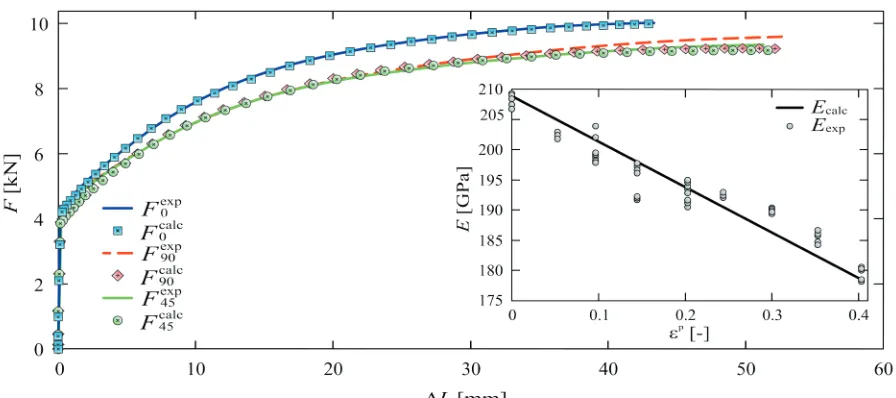
The established F – ΔL relationships for the three
considered directions, which include the rolling direction (0°), transverse direction (90°) and diagonal direction (45°), are graphically displayed in Fig. 1.
From three hardening curves which are displayed in Fig. 1, one can observe that cold rolled metal sheet EN 1.4301 exhibits a significant degree of plastic anisotropy, which certainly cannot be neglected in numerical simulations.
Fig. 1. Tensile test measurements
2.2 Effective Young’s Modulus Degradation
The degradation of the effective Young’s modulus was measured as a function of the longitudinal plastic strain, which can be defined for the uniaxial stress case as εp = ln ((L0 + ΔL) / L0). The corresponding
experimental procedure is a two-stage loading procedure in which standard specimens are first plastically prestrained in the tensile test machine to a certain degree of the equivalent plastic strain and then released. The thickness and width of each prestrained specimen is precisely measured in order to evaluate the respective cross-sectional area which will be needed in subsequent stiffness analysis. In the second stage, each plastically prestrained specimen is clamped again in the tensile test machine and loaded only elastically. In order to accurately follow the elastic response, the machine is equipped with a precise dynamometer, which can measure force in a range up to ±10 kN with accuracy class being 1 (ISO 376, EN 10002–3), whereas the strain transducer, which is mounted on the specimen as shown in Fig. 2, is of accuracy class 0.1 while its nominal displacement range is ±2.5 mm.
From the measured force-displacement relationship registered by elastic loading and
unloading of the plastically prestrained specimen, the effective elastic modulus can be calculated considering Hooke’s law by using the interpolation of the measurement data of length, cross-sectional area, and force. In order to retrieve the effective Young’s modulus degradation as a function of the longitudinal plastic strain, the described procedure is repeated for different degrees of the applied plastic prestrain. As can be clearly seen from the plotted graph in Fig. 3, it is beyond all question that the evidenced degradation of the effective Young’s modulus is directly correlated to the degree of the applied plastic prestrain. The fact that, in our experiment, plastic prestraining was achieved under the condition of a uniaxial stress state certainly does not affect the general statement. The phenomenon described here can be found also in [22] and [23].
Fig. 2. Measurement of elastic elongation
Fig. 3. Young’s modulus degradation due to plastic straining
3 IDENTIFICATION OF THE PARAMETERS
[24] and [25]. The goal of the optimization is to fit with the respective numerical simulation, when performed by considering the GHM model, the performed experiments to a greatest extent. Thus, in the optimization, the model parameters that are under consideration take the role of design variables, while the cost function to be minimised is defined as the discrepancy between the numerical and experimental responses. With a corresponding adjustment of the model parameters’ values, we have thus tried to numerically obtain both the measured
force-displacement curve (F – ΔL) in three observed
directions (0, 45, and 90°) and the measured effective Young’s modulus degradation at the same time.
Parameters q1, q2 and q3 are essentially an
improvement of the basic Gurson’s constitutive model, upgrading thus the original plastic potential [9]. Since the values of those parameters are similar for all metals [6], we adopt them by taking q1 = 1.5,
q2 = 1 and q3=q12=2 25. . Further, we have observed
that the model fits more adequately the measured
effective Young’s modulus degradation when An in
Eq. (9) does not follow the normal distribution. Thus, An has been adopted as the independent parameter of
the model; in that case only one parameter needs to be identified instead of three. Also, considering specific of the planar anisotropy in the rolled sheet only two yield stress ratios, R22 and R12, have been chosen as
relevant for the characterization of the anisotropic behaviour (parameters of Hill48). Accordingly, only R22 and R12 have been identified, whereas the
remaining yield stress ratios were set to 1.
Further, the control points σMε =σ εM( )Mp of the
cubic spline, which is used for the definition of the
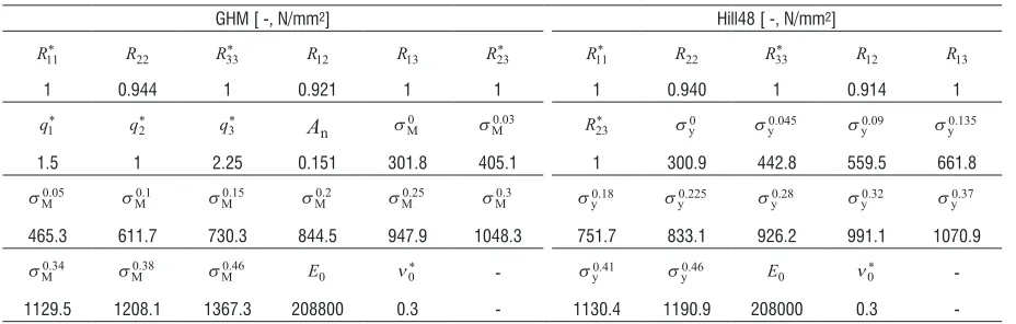
hardening behaviour, have been the subject of the identification as well. Values of all the GHM model parameters, those that are identified and those that are assumed, are tabulated in Table 1. The values, which are denoted in the table by an asterisk, are assumed to be fixed and are not subject to identification.
As can be seen from Fig. 4, a very good agreement
between the calculated and measured F – ΔL curves
and the effective Young’s modulus degradation as a function of the elongation of gauge length is obtained for the optimised GHM model.
To provide elements for a comparative analysis between different constitutive models, the same procedure for the parameters’ identification has been used for Hill48 model, but considering a reduced experimental data set. In the Hill48 model parameters identification, only the deviation in F – ΔL curves is considered as the cost function. The corresponding parameter values for the Hill48 constitutive models are
tabulated in Table 1, where σε σ ε
y = y( )eqp represents the control points of the cubic spline for the definition of the hardening behaviour.
4 VALIDATION OF THE MODEL ON SPRINGBACK TEST
introduce geometrically defined longitudinal plastic strain εp
0 0
=ln(( + )/ )L ∆L L , which is defined with the elongation of the respective gauge length. Such plastically prestrained specimens are then clamped, in the second part of the experiment, into a special bending tool (Fig. 5a) and subsequently bent in an angle of γ = 90° (Fig. 5b). As a result, the initially homogeneous plastic strain state, which is due to the applied plastic prestrain in the first part of the experiment, is now subject to change into a non-homogeneous one because of the developed plastic strains by bending.
Nevertheless, the applied plastic prestrain and its amount still has a decisive role in the resulting non-homogeneous plastic strain and stress distribution, which will be clearly seen from the exhibited springback behaviour (Fig. 5c).
Lastly, in the considered experiment, after the removal of the bending load and re–established equilibrium of the bent specimen under residual stresses, its deviation from perpendicularity (γ = 90°), denoted in Fig. 5a by angle α, is measured. In fact, in this experiment, the angle α is a clearly visible measure of the exhibited springback behaviour of the bent steel sheet. From a photograph of one set of the bent specimens, shown in Fig. 5c, one can clearly see how the degree of plastic prestrain is directly related to the intensity of the exhibited springback. More extensive springback, which is evidenced with a larger amount of plastic prestrain, may be attributed to the following: greater actual yield stress due to the occurred hardening, thinner specimens, and lower effective Young's modulus. All of these effects are a direct consequence of the previous plastic prestraining, with their variation being proportional in a non-linear way to the degree of the applied plastic prestrain.
Fig. 5. Springback test; bending of prestrained specimens; a) experiment, b) simulation, c) bent specimens
Table 2. Comparison of the springback angle, experiment vs. calculations (rolling direction)
prestrain εp
[-] in rolling direction
angle α [°] bending in rolling direction
experimental numerical GHM Hill48 0 10.3 10.2 10.2 0.053 13.9 14.2 14.0 0.097 17.4 17.4 16.9 0.144 20.8 20.5 19.6 0.203 24.8 24.1 22.7 0.244 26.8 26.1 25.3 0.300 30.4 30.3 27.9 0.353 33.1 33.5 30.7 0.402 36.8 36.6 33.5
The measured springback angle α is then compared in the validation test with the results obtained by a numerical simulation of the considered springback test. The computer simulation is based
Table 1. Values of the identified and assumed fixed parameters
GHM [ -, N/mm2] Hill48 [ -, N/mm2]
R11* R22 R33* R12 R13 R23* R11* R22 R33* R12 R13
1 0.944 1 0.921 1 1 1 0.940 1 0.914 1
q1* q2* q3* An σM0 σM0 03. R23* σy0 σy0 045. σy0 09. σy0 135.
1.5 1 2.25 0.151 301.8 405.1 1 300.9 442.8 559.5 661.8
σM0 05. σ
M0 1. σM0 15. σM0 2. σM0 25. σM0 3. σy0 18. σy0 225. σ0 28y. σy0 32. σy0 37.
465.3 611.7 730.3 844.5 947.9 1048.3 751.7 833.1 926.2 991.1 1070.9
σM0 34. σ M
0 38. σ
M0 46. E0 ν0* - σy0 41. σy0 46. E0 ν0*
-on the FEM code ABAQUS/Explicit by using the VUMAT subroutine for the implementation of the GHM model. In the simulation, 100 shell elements with a reduced integration (S4R) and 11 through thickness section points were used to model the specimen, while the tools were assumed to be rigid. The results of the calculated and measured springback angle a for the ‘rolling direction specimens’ are presented in Table 2, whereas in Table 3, the respective springback angle α values for the ‘transverse direction specimens’ are displayed.
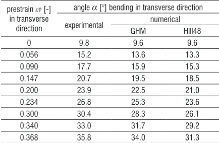
Table 3. Comparison of the springback angle, experiment vs. calculations (transverse direction)
prestrain εp [-] in transverse
direction
angle α [°] bending in transverse direction
experimental numerical GHM Hill48
0 9.8 9.6 9.6
0.056 15.2 13.6 13.3 0.090 17.7 15.9 15.3 0.147 20.7 19.5 18.5 0.200 23.9 22.5 21.0 0.234 26.8 25.3 23.6 0.300 30.4 28.3 26.1 0.340 33.0 31.7 29.2 0.368 35.8 34.0 31.3
From Tables 2 and 3, it can be seen that the approach presented here, which is formulated as the GHM model, gives much more accurate results. From the histograms, plotted in Figs. 6 and 7, showing for both considered constitutive models the respective absolute value of the established relative deviations between the simulated and the experimental springback, the advantage of the GHM model is even more distinct.
It is beyond all doubt that the overall departure of the calculated springback from the experimental one is smaller when the GHM model is used in comparison with the Hill48 model. Nevertheless, some further detailed perceptions can be extracted from the obtained results:
• When plastic prestraining in the rolling direction is small, both of the constitutive models that are considered here give similar results because the stiffness degradation is negligible and anisotropy has a minor influence.
• At a higher degree of plastic prestraining in the
rolling direction, however, the Hill48 model underestimates springback, as is seen in Table 2. The main cause lies in the fact that it neglects the degradation of the effective Young’s modulus.
There, the advantage of the GHM model becomes visible.
• The deviations from the experimental evidence
are larger in the case of prestraining in the transverse direction for both models. The error may be attributed to the adoption of the isotropic evolution of the stiffness degradation in the GHM model and the adoption of the Hill48 anisotropy, the latter having limited possibility of anisotropy modelling due to its simplicity. Nevertheless, the springback prediction with the GHM model is, again, much more precise than the classical approach.
Fig. 6. Absolute value of relative deviations of springback (rolling direction)
Fig. 7. Absolute value of relative deviations of springback (transverse direction)
5 CONCLUDING REMARKS
simultaneous modelling of the stiffness degradation and anisotropy can be a true key for resolving the problem of physically reliable simulation of springback. It is clearly seen from the obtained results that, in the calculations of springback, neither stiffness degradation nor anisotropy in sheet metal should be neglected. One way to take those effects into account is the approach elaborated and validated in this article, which has resulted in the so-called GHM model. Although the stiffness degradation due to occurrence of damage could be tackled in a much more sophisticated way (which is, however, a matter of further research), the approach used with the effective Young’s modulus degradation considered covers the phenomenological background adequately enough to qualitatively demonstrate its impact on the numerical springback behaviour.
6 ACKNOWLEDGEMENT
The authors would like to express their gratitude to the
company Kovinoplastika Lož d.d., which enabled the
experimental research that is presented in the paper, and to the Slovenian Research Agency for its financial support.
7 REFERENCES
[1] Geng, L.M., Shen, Y., Wagoner, R.H. (2002). Anisotropic hardening equations derived from reverse-bend testing. International Journal of Plasticity, vol. 18, no. 5-6, p. 743-767.
[2] Chun, B.K., Kim, H.Y., Lee, J.K. (2002). Modeling the Bauschinger effect for sheet metals, part II: applications. International Journal of Plasticity, vol. 18, no. 5-6, p. 597-616.
[3] Bonora, N., Gentile, D., Pirondi, A., Newaz, G. (2005). Ductile damage evolution under triaxial state of stress:
theory and experiments. International Journal of
Plasticity, vol. 21, no. 5, p. 981-1007, DOI:10.1016/j.
ijplas.2004.06.003.
[4] Vrh, M., Halilovic, M., Stok, B. (2008). Impact of Young’s modulus degradation on springback calculation in steel sheet drawing. Strojniski vestnik -
Journal of Mechanical Engineering, vol. 54, no. 4, p.
288-296.
[5] Halilovic, M., Vrh, M., Stok, B. (2009). Prediction of elastic strain recovery of a formed steel sheet considering stiffness degradation. Meccanica, vol. 44, no. 3, p. 321-338, DOI:10.1007/s11012-008-9169-8.
[6] ABAQUS. (2008). User’s Manual, Ver. 6.7. Simulia,
Providence.
[7] Kachanov, L.M. (1958). Rupture time under creep conditions. Otdelenie techniceskih Nauk, Izvestiya Akademii Nauk SSSR, vol. 8, p. 26-31 (in Russian).
English translation (1999): Rupture time under creep conditions. International Journal of Fracture, vol. 97, no. 1-4, p. 11-18.
[8] Gurson, A.L. (1977). Continuum theory of ductile rupture by void nucleation and growth 1. Yield criteria
and flow rules for porous ductile media. Journal of
Engineering Materials and Technology-Transactions of
the ASME, vol. 99, no. 1, p. 2-15.
[9] Tvergaard, V. (1981). Influence of voids on shear band instabilities under plane-strain conditions. International
Journal of Fracture, vol. 17, no. 4, p. 389-407,
DOI:10.1007/BF00036191.
[10] Chu, C.C., Needleman, A. (1980). Void nucleation
effects in biaxially stretched sheets. Journal of
Engineering Materials and Technology-Transactions
of the ASME, vol. 102, no. 3, p. 249-256,
DOI:10.1115/1.3224807.
[11] Mori, T., Tanaka, K. (1973). Average stress in matrix and average elastic energy of materials with misfitting inclusions. Acta Metallurgica, vol. 21, no. 5, p. 571-574, DOI:10.1016/0001-6160(73)90064-3.
[12] Benzerga, A.A., Besson, J. (2001). Plastic potentials
for anisotropic porous solids. European Journal of
Mechanics - A/Solids, vol. 20, no. 3, p. 397-434,
DOI:10.1016/S0997-7538(01)01147-0.
[13] Zhao, Y.H., Tandon, G.P., Weng, G.J. (1989).
Elastic-Moduli for a class of porous materials. Acta
Mechanica, vol. 76, no. 1-2, p. 105-130, DOI:10.1007/
BF01175799.
[14] Hu, G.K., Weng, G.J. (2000). Some reflections on the Mori-Tanaka and Ponte Castaneda-Willis methods
with randomly oriented ellipsoidal inclusions. Acta
Mechanica, vol. 140, no. 1-2, p. 31-40.
[15] Riccardi, A., Montheillet, F. (1999). A generalized self-consistent method for solids containing randomly oriented spheroidal inclusions. Acta Mechanica, vol. 133, no. 1-4, p. 39-56, DOI:10.1007/BF01179009. [16] Eshelby, J.D. (1957). The determination of the elastic
field of an ellipsoidal inclusion, and related problems.
Proceedings of the Royal Society, vol. 241, no. 1226, p.
376-396, DOI:10.1098/rspa.1957.0133.
[17] Carvalho, F.C.S., Labuz, J.F. (1996). Experiments on effective elastic modulus of two-dimensional solids with cracks and holes. International Journal of
Solids and Structures, vol. 33, no. 28, p. 4119-4130,
DOI:10.1016/0020-7683(95)00269-3.
[18] Pundale, S.H., Rogers, R.J., Nadkarni, G.R. (1998). Finite element modeling of elastic modulus in ductile irons: Effect of graphite morphology. AFS Transactions, vol. 106, p. 99-105.
[19] Bohm, H.J., Eckschlager, A., Han, W. (2002). Multi-inclusion unit cell models for metal matrix composites with randomly oriented discontinuous reinforcements.
Computational Materials Science, vol. 25, no. 1-2, p.
42-53, DOI:10.1016/S0927-0256(02)00248-3.
[20] Halilovic, M., Vrh, M., Stok, B. (2009). NICE-An explicit numerical scheme for efficient integration of
Computers in Simulation, vol. 80, no. 2, p. 294-313, DOI:10.1016/j.matcom.2009.06.030.
[21] Vrh, M., Halilovic, M., Stok, B. (2010). Improved explicit integration in plasticity. International Journal
for Numerical Methods in Engineering, vol. 81, no. 7,
p. 910-938.
[22] Morestin, F., Boivin, M. (1996). On the necessity of taking into account the variation in the Young modulus with plastic strain in elastic-plastic software. Nuclear
Engineering and Design, vol. 162, no. 1, p. 107-116,
DOI:10.1016/0029-5493(95)01123-4.
[23] Yang, M., Akiyama, Y., Sasaki, T. (2004). Evaluation of change in material properties due to plastic deformation.
Journal of Materials Processing Technology,
vol. 151, no. 1-3, p. 232-236, DOI:10.1016/j. jmatprotec.2004.04.114.
[24] Levenberg, K. (1944). A method for the solution of certain non-linear problems in least squares. The
Quarterly of Applied Mathematics, vol. 2, no. 2, p.
164-168.
[25] Marquardt, D. (1963). An algorithm for least-squares
estimation of nonlinear parameters. Journal of the
Society for Industrial and Applied Mathematics,