Optimization of a Product Batch Quantity

0 INTRODUCTION

The goal of calculating the optimal batch quantity of a product is that the product is produced in the required quantity and required quality at the lowest cost [1] to [3].

There are basically two options of planning the batch quantity [4]:

• planning a large batch of a product in long

intervals,

• planning a small batch of a product in short

intervals.

The advantages of planning a large batch of product are:

• price advantage of ordering a large batch (low cost, protection against raising prices, volume rebate),

• lower administrative costs,

• lower costs of tests and shipping,

• low risk of interruption of production because of the large stock.

The disadvantages of planning a large batch are:

• high tied-up capital,

• high storage costs of product inventory.

The advantages of planning a small batch of product are:

• low tied-up capital,

• low storage costs of product inventory,

• high flexibility if quantities change at

suppliers and buyers.

The disadvantages of planning a small batch are:

• the costs of frequent ordering,

• high risk of interruption of production because of a small product inventory.

Somewhere between the large and small batch quantity is the optimal batch quantity, i.e. the quantity in which the cost per product unit is the lowest.

Aggterleky [4] describes the optimal planning planes and the meaning of under- and over planning, and the influence of the reduction of total cost. Wiendahl [5] uses Harris and Andler’s equation for the determination of the optimal quantity. Härdler [6] takes into account the costs of storage and delivery in determining the optimal batch quantity. Muller [7] and Piasecki [8] assert that inventory management is explained only with the basics of an optimal quantity calculation. So, in comparison to the aforementioned papers, where only the determination of the optimum quantity is given, our model is expanded to include the impact of the flow time on the batch quantity or stock.

1 ECONOMIC ORDER QUANTITY – BASIC MODEL

Changing the product batch (hereinafter referred to as ‘order’) causes two types of costs [9]:

• order change costs,

• storage costs.

Order change costs include costs for preparing documentation, costs of control and input of goods, costs of workers’ wages, costs of setting up the machines, and costs of producing samples.

The order, therefore, causes annual costs, known as order change costs SMen. The higher the ordered

quantity is, the lower the influence of the order change costs is (Fig. 1a). The order also causes storage costs, which include the costs of interest on the bound capital and warehouse costs.

The order therefore also causes annual storage costs SSkl, which increase proportionally as the ordered quantity increases (Fig. 1b).

The sum of the annual order change costs and storage costs has the minimum value of the total costs SVso,min at the optimal batch quantity xOpt (basic

model) (Fig. 1c).

Optimization of a Product Batch Quantity

Berlec, T. – Kušar, J. – Žerovnik, J. – Starbek, M.

Tomaž Berlec* _{– Janez Kušar – Janez Žerovnik – Marko Starbek}

University of Ljubljana, Faculty of Mechanical Engineering, Slovenia

Companies encounter various challenges when entering the global market, one of the most significant being the calculation of the optimal batch quantity of a product. This paper explains how to calculate the optimal batch quantity using first the basic model, and then the extended model that takes into account the tied-up capital in a production, in addition to the costs of changing the batch and storage costs. There is a case study of calculating the optimal batch quantity using the basic and extended models, together with conclusions regarding when either of the two models should be used. For optimal batch quantities we also calculated lead times, corresponding costs of tied-up capital per piece, and the difference between costs per piece when using the basic and extended models.

The optimal batch quantity in the basic model [6] and [7] can be calculated by using the following sequence of steps:

Step 1: Calculation of annual order change costs:

S L

x s

Men = ⋅ Men, (1)

where SMen are annual order change costs [€/a], L

annual needs [piece/a], x batch quantity [piece], and

sMen order change costs [€].

Step 2: Calculation of annual storage costs: Pulse inflow and steady outflow of goods is assumed (Fig. 2). The annual storage costs depend on the warehouse inventory:

S = x s_{Skl Obd} p

2⋅ ⋅ , (2)

where SSkl are storage costs [€/a], x batch quantity

[piece], sObd processing costs per piece [€/piece], and

p interest rate of tied-up capital [1/a].

Step 3: Calculation of total annual order costs:

S = S + S = L

x s + x s p

Vso Men Skl ⋅ Men ₂⋅ Obd⋅ . (3) Step 4: Calculation of economic order quantity

xOpt:

The economic order quantity (i.e. the minimum value of this function) can be found by differentiation.

Differentiating SVso with respect to x and then equating to zero, we get:

d

d .

S

x = Lx s

s _{p =}

Vso

Men Obd

− ₂⋅ + ⋅

2 0

The optimal batch quantity xOpt:

x = L s

s p

Opt Men

Obd

2⋅ ⋅

⋅ , (4)

where xOpt are optimal batch quantity [piece], L annual

needs [piece/a], sMen order change costs [€], sObd

Fig. 1. a) order change costs, b) Storage costs of order, c) Optimal batch quantity xOpt in the basic model

processing costs per piece [€/piece], and p interest rate of tied-up capital [1/a].

The interest rate of tied-up capital p is calculated on the basis of the bank interest rate for a long-term loan with additional interest using the VDI 3330 guidelines (Table 1).

Table 1. Interest rate of tied-up capital, in [%]

A. Bank interest rate for a long-term capital loan 7.15 Additional interests:

limitation 3 to 5

losses caused by break or rupture 2 to 4

transport 2 to 4

storage and write-off 1.5 to 2

warehouse management 1 to 2

control 1 to 2

insurance 0.5 to 1

B. SUM OF ADDITIONAL INTERESTS 11 to 20 INTEREST RATE OF TIED-UP CAPITAL p = A + B 18.15 to 27.15

2 ECONOMIC ORDER QUANTITY – EXTENDED MODEL

In our basic model for the calculation of optimal batch quantity only the order change costs SMen and storage

costs SSkl were taken into account.

Analysis of the diagram of the flow of orders through work systems [10] revealed that during the processing of the observed order in a given workplace, other orders have to wait for the release of capacities, which in turn causes additional costs related to the tied-up capital in production (Fig. 3).

Fig. 3. Flow diagram showing inventory of orders

Tying-up the capital in the material flow from a supplier through production to the customer [11] is shown in Fig. 4.

After having carried out an analysis of the flow diagram showing the status of orders, and a diagram of tying-up the capital on the path from supplier to customer, Nyhuis and Fronla [12] concluded that when calculating the economic order quantity, in addition to

the cost of order change SMen and storage costs SSkl,

it would also be necessary to take into account the costs of execution of operations of an order in the production SIzv and costs of disposal (transition) SPre.

Fig. 4. Tying-up the capital in the material flow from supplier to customer

The optimal batch quantity in the extended model

xOpt* will be the one in which the sum of annual order

change costs, the storage costs, the costs of execution of operations of an order, and the transition costs will have the minimum value (Fig. 5).

Fig. 5. Optimal batch quantity xOpt* in the extended model

The optimal batch quantity xOpt* in the extended

model is calculated in the following sequence:

Step 1: Calculation of annual order change costs:

S L

x s Men *

* Men

= ⋅ ,

where SMen* are annual order change costs [€/a], L

annual needs [piece/a], x* _{batch quantity [piece], sMen}

Step 2: Calculation of annual storage costs: Pulse inflow and steady outflow of goods is assumed (Fig. 3). The annual storage costs are:

p s x

S_Skl= ⋅ _Obd⋅

2

*

* _,

where SSkl* are annual storage costs [€/a], x* batch

quantity [piece], sObd processing costs per piece [€/

piece], p interest rate of tied-up capital [1/a].

Step 3: Calculation of annual costs of order-processing times:

The one-dimensional lead time of an order operation, consisting of the turnaround time of the operation TIzv and the interoperation time TPre is shown in Fig. 6 [10].

Fig. 6. Lead time of operation; Tp setup time [min],

tObd manufacturing time [min], TIzv turnaround time [day],

TPre interoperation time [day], TO lead time of operation [day]

Known order-processing times allow for a calculation of annual costs due to operation-execution times SIzv* :

S = (s s ) L p

RC T

Izv

* Mat Obd

Izv

+ ⋅ ⋅

⋅ ⋅

∑

2 , (5)

where SIzv* are annual costs arising from the

operation-execution of an order [€/a], sObd processing costs per piece [€/piece], sMat material costs per piece [€/piece], L annual needs [piece/a], p interest rate of tied-up capital [1/a], RC available time [day/a], ΣTIzv total

operation-execution time [day].

Step 4: Calculation of annual costs due to interoperation time:

S = (s s ) L p

RC T

e

* Mat Obd

e

Pr Pr ,

+ ⋅ ⋅

⋅ ⋅

∑

2 (6)

where S*Pre are annual costs due to interoperation time [€/a], and ΣTPre sum of interoperation times [Wd].

Step 5: Calculation of total annual costs SVso* : S = S_Vso* S S S

Men * Skl * Izv * e *

+ + + _Pr , (7)

S = L

x s x s p

s s L p

RC T

s Vso* * Men

* Obd Mat Obd Izv Ma ⋅ + ⋅ ⋅ + + + ⋅ ⋅ ⋅ ⋅ + +

∑

2 2 ( )

( tt Obd

e

s L p

RC T + ⋅ ⋅ ⋅ ⋅

∑

) _, Pr 2 S L

x s x s p

s s L p

RC T T

Vso* * Men * Obd Mat Obd Izv e = ⋅ + ⋅ ⋅ + +

(

+

)

⋅ ⋅ ⋅ ⋅

∑

+

∑

2

2  Pr .

(8)

The material flow rate ST is defined by the Eq (9):

ST = T T

T

Izv e

Izv

∑

+

∑

_Pr

. (9)

Therefore, Eq. (9) can be transformed to:

T

∑

_Izv+

∑

T_Pre=ST⋅

∑

T_Izv. (10) The total time of the operation-execution of an order is defined as:

T = T x t

KAP

Izv p

* e

∑

∑

+ ⋅_⋅ 1

60 , (11)

where ΣTIzv is total time of operation execution of an

order [day], Tp setup time [min], te1 time per unit [min/

piece], KAP daily capacities [h/day], x* _{batch quantity}

[piece].

If Eqs. (10) and (11) are inserted in Eq. (8), the function for calculating the total order-dependent costs is transformed to:

S = L

x s x s p

(s s ) L p

RC ST

T x t Vso* * Men

* Obd

Mat Obd p * e

⋅ + ⋅ ⋅ + + + ⋅ ⋅ ⋅ ⋅ ⋅ + ⋅ 2 2 11 60⋅

∑

_KAP ,

Step 6: Calculation of the economic order quantity x_Opt* _:

The minimum value of the function S_Vso* _{can be}

found by differentiation. Differentiating SVso* with

respect to x* _{and then equating to zero, we get:} dS

dx = - L_x s

s p

(s s ) L p

RC ST

t Vso*

* _* Men Obd

Mat Obd e

( )

⋅ + ⋅ + + + ⋅ ⋅ ⋅ ⋅ ⋅ 2 1 2

2

60

2 1

⋅

( )

⋅ ⋅ + + ⋅ ⋅ ⋅ ⋅ ⋅

∑

L

x s = s p (s

s ) L p

RC ST

t KAP

* Men Obd

Mat Obd e _.

The economic order quantity (i.e. optimal batch quantity) is therefore:

x L s

s p ST

Opt

* Men

Obd (sMat sObdRC) L p KAPte

= ⋅ ⋅

⋅ + + ⋅ ⋅ ⋅ ⋅

⋅

∑

2

60 1

. (12)

where x_Opt* _{is optimal batch quantity [piece], L annual}

needs [piece/a], sMen order change costs [€], sObd

processing costs per piece [€/piece], p interest rate of tied-up capital [1/a], sMat material costs per piece [€/

piece], RC available time [day/a], ST material flow

rate, te1 time per unit [min/piece], KAP daily capacities [h/day].

These models are applicable when there is no fluctuation on the relation market-producer. There are neither distributions of production and demand processes considered nor the stochastic character of the mentioned processes.

3 CASE STUDY OF CALCULATING THE OPTIMAL BATCH QUANTITY OF A PRODUCT

Company X, which is a supplier to a car components manufacturer, found it increasingly difficult to be competitive on the global market due to excessively long manufacturing lead times and too high product prices.

The company’s management organised a creativity workshop [13] to [15] in order to identify urgent measures, whose implementation would improve their market competitiveness.

The results of the creativity workshop showed that it would be necessary to do the following in the company:

• significantly reduce the inventory in entry and exit warehouses, and on disposal locations within the production,

• significantly reduce the lead times of orders. After the presentation of the results of the creativity workshop, management decided that they would first solve the problem of large stocks (i.e. tied-up capital), which significantly raise the price of products (i.e. non-competitiveness) [16] to [18].

A project team was established in the company, in order to analyse the causes of large stocks and to propose possible solutions.

Team members analysed inventories in all warehouses. Together with the heads of warehouses

and the planners of production, they concluded that the batch quantities are defined on the basis of the experience of planners (i.e. estimates), which lead either to excessive stocks or a shortage of goods.

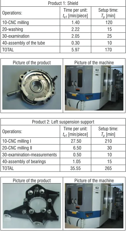
Product 1: Shield

Operations: _tTime per unit: e1[min/piece]

Setup time: Tp [min]

10-CNC milling 1.40 120

20-washing 2.22 15

30-examination 2.05 25

40-assembly of the tube 0.30 10

TOTAL 5.97 170

Picture of the product Picture of the machine

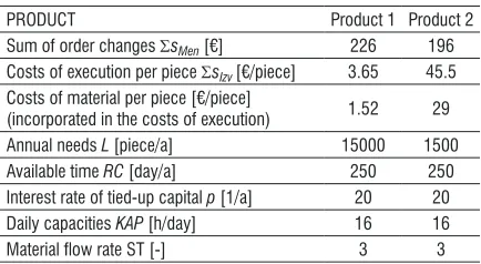
Product 2: Left suspension support

Operations: _tTime per unit: e1[min/piece]

Setup time: Tp [min]

10-CNC milling I 27.50 210

20-CNC milling II 6.50 30

30-examination-measurements 0.50 10 40-assembly of bearings 1.05 15

TOTAL 35.55 265

Picture of the product Picture of the machine

Fig. 7. te1and Tp times for shield and suspension support The project team contacted the experts for help in solving the problem of over- and understocking of goods. Experts suggested that project team could use Eqs. (4) and (12) in order to calculate the optimal batch quantities of products.

The project team decided that the first experimental calculation of the optimal batch quantity would be carried out for two products:

• Product 1: Shield;

• Product 2: Left suspension support.

The project team obtained the following data from the technology routings for both products:

• Data on times per unit te1 and setup times Tp (Fig.

7).

• Other data, required for calculation of optimal product batch (Table 2), were obtained from various departments in the company.

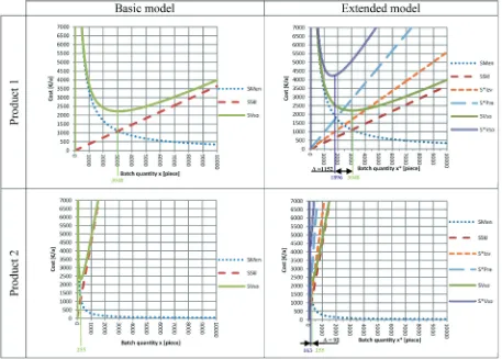
Table 2. Data from company departments

PRODUCT Product 1 Product 2

Sum of order changes SsMen [€] 226 196 Costs of execution per piece SsIzv[€/piece] 3.65 45.5 Costs of material per piece [€/piece]

(incorporated in the costs of execution) 1.52 29

Annual needs L [piece/a] 15000 1500

Available time RC [day/a] 250 250

Interest rate of tied-up capital p [1/a] 20 20

Daily capacities KAP [h/day] 16 16

Material flow rate ST [-] 3 3

In order to assess the usability of the basic and extended model for the calculation of optimal batch quantity for both products, the project team decided that it would carry out the following:

• Calculation of optimal batch quantity for Products 1 and 2 using the basic and extended model:

• basic model:

x = L s

s p

Opt Men

Obd

2⋅ ⋅ ⋅ ,

• extended model:

x L s

s p ST

Opt

* Men

Obd (sMat sObdRC) L p KAPte

= ⋅ ⋅ ⋅ + + ⋅ ⋅ ⋅ ⋅ ⋅

∑

2 60 1 .

• Calculation of batch lead times for Products 1 and 2 using the basic and extended model:

• basic model:

TO = ST ∙ TIzv , T = T t x

KAP Izv

p+ ⋅e Opt

(

)

⋅

∑

1

60 ,

• extended model:

TO* = ST ∙ TIzv* , T = T t x KAP Izv

p e Opt * * . + ⋅

(

)

⋅

∑

1 60

• Calculation of costs per product unit using the basic and extended model:

• basic model:

s = s s s s

x

Kos Obd To e Men

Opt

+ + _Pr + ,

where sKos are costs per product unit [€/piece], sTo costs of tied-up capital per product unit during the lead time [€/piece], and sPre costs of tied-up

capital per product unit during interoperation time [€/piece],

s = s s p T

RC

To Mat Obd O

+

(

)

⋅

⋅

2 , s =

s p x

L

e Obd Opt

Pr ,

⋅ ⋅ ⋅

2

• extended model:

s = s s s s

x

Kos Obd To e Men

Opt * * * Pr * * , + + +

s = (s s ) p T RC To

* Mat+ Obd ⋅ _⋅ O*

2 , s =

s p x

L e

* Obd Opt*

Pr .

⋅ ⋅ ⋅

2

• Calculation of difference of costs per product unit:

∆s = s_{Kos Kos−}s*_Kos.

The calculations were made with MS Excel software. The results are shown in Table 3.

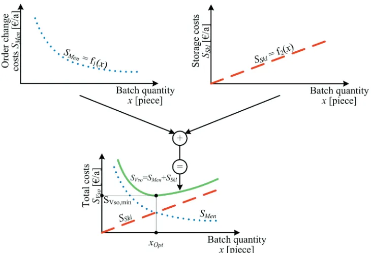
The project team charted the influence of the batch quantity on the product costs (Fig. 8).

The results listed in Table 3 and Fig. 8 led the project team to the following conclusions:

• The calculated optimal batch quantities of both products are significantly different from the current estimated batch quantities. Due to this fact, the storage costs are high.

• Batch lead times are too long.

• The technology routing of Product 1 defines

the short times per unit te1; diagrams on Fig. 8 show that at the transition from the basic to the extended model for calculation of the optimal batch quantity, the batch quantity is only slightly reduced and the total costs of tied-up capital are only slightly higher (if the total time te1 is small, the basic model can be used for calculation of optimal batch quantity).

is large, extended model must be used for the calculation of optimal batch quantity).

• The basic model for calculation of optimal batch quantity does not take into account the tying-up of capital in production, and thus the optimal batch quantities are bigger than in the extended model.

Table 3. Results of calculations of optimal batch quantities for both products

CALCULATION

Product 1: SHIELD

Product 2: SUSPENSION

SUPPORT

Model Model

Basic Extended Basic Extended Optimal batch quantity x

[piece] 3048 1896 255 163

Batch lead time TO [day] 57.40 35.90 38.88 25.25 Costs per product unit sKos

[€/piece] 3.92 3.89 48.20 47.95

Difference of costs per

product unit SsKos [€/piece] 0.03 0.25

At the presentation of results, the company management agreed that the project team would continue its work in order to reduce lead times of orders.

4 CONCLUSION

This paper explains how to calculate the optimal batch quantity of a product (production is within the company) using the known basic and developed extended models; the latter, in addition to the costs of changing the batch (i.e. order) and storage costs, also takes into account the costs of interoperation time and the costs of execution of operations.

The project team in the company, which is a supplier of car components manufacturer, carried out some experiments, whose results have shown when to use the basic model and when to use the expanded model for the calculation of the optimal batch quantity. Further experiments in electro-mechanical industry will be needed for reliable decision making regarding the selection of the basic or extended model.

The model also needs to be further developed requiring a connection between the optimal quantities procuring materials in warehouses.

The company management decided for the project team to carry out also an AS-IS analysis of value flow for existing batch quantities. After a transition to optimal batches, the project team will repeat the value flow analysis for the same two products and find lead-time savings.

5 REFERENCES

[1] Heizer, J., Render, B. (2001). Principles of Operations

Management, 6th _{ed., Prentice Hall, Upper Saddle}

River.

[2] Fogarty, W.D., Blackstone, H.J., Hoffman, R.T. (1991).

Production and Inventory Management (2nd _ed.).

Cengale Learning, Stamford.

[3] Slack, N., Chambers, S., Harland, C., Harrison, A., Johnson, R. (1995). Operations Management. Pitman Publishing, London.

[4] Aggteleky, B. (1990). Fabrikplanung, Band 3, Carl Hanser Verlag, München, Wien.

[5] Wiendahl, H.P. (2008). Betriebsorganistion für Ingenieure. Carl Hanser Verlag, München, Wien.

[6] Härdler, J. (2012). Betriebswirtschaftslehre für Ingenieure. Carl Hanser Verlag, München, Wien. [7] Muller, M. (2011). Essentials of Inventory Management,

2nd _{edition, Amacom, New York.}

[8] Piasecki, D.J. (2009). Inventory Management Explained: A Focus on Forecasting, Lot Sizing, Safety Stock, and Ordering Systems. Ops Publishing, Kenosha. [9] Vollman, E.T., Berry, L.W., Whybark, D.C., Jacobs,

F.R. (2005). Manufacturing Planning and Control Systems. McGrow-Hill, New York.

[10] Wiendahl, H.P. (1994). Load-Oriented Manufacturing Control. Springer-Verlag, London.

[11] Arnold, D., Furmans, K. (2009). Materialfluss in Logistiksystemen. Springer Verlag, Heidelberg, DOI:10.1007/978-3-642-01405-5.

[12] Nyhuis, P., Fronla, P. (2012). Durchlauforientierte Lösgrössenbestimmung, from http://www. enzyklopaedie-der-wirtschaftsinformatik.de/, accessed at 2012-01-19.

[13] Rihar, L., Kušar, J., Duhovnik, J., Starbek, M. (2010). Teamwork as a Precondition for Simultaneous Product

Realization. Concurrent Engineering: Research and

Applications, vol. 18, no. 4, p. 261-273, DOI:10.5545/ sv-jme.2012.420.

[14] Kušar, J., Berlec, T., Žefran, F., Starbek, M. (2010).

Reduction of Machine Setup Time. Strojniški vestnik – Journal of Mechanical Egineering, vol. 56, no. 12, p. 833-845.

[15] Rihar, L., Kušar, J., Gorenc, S., Starbek, M. (2012). Teamwork in the Simultaneous Product Realisation. Strojniški vestnik – Journal of Mechanical Egineering, vol. 58, no. 9, p. 534-544.

[16] Buchmeister, B., Pavlinjek, J., Palčič, I., Polajnar, A.

(2008). Bullwhip Effect Problem in Supply Chains. Advances in production engineering & management, vol. 3, no. 1, p. 45-55.

[17] Palčič, I., Buchmeister, B., Polajnar, A. (2010). Analysis

of Innovation Concepts in Slovenian Manufacturing Companies. Strojniški vestnik – Journal of Mechanical Egineering, vol. 56, no. 12, p. 803-810.

[18] Božičković, R., Radošević, M., Ćosić, I., Soković, M., Rikalović. A. (2012). Integration of Simulation