Desert
Online at http://desert.ut.ac.ir
Desert 24-1 (2019) 119-132
Comparing pixel-based and object-based algorithms for
classifying land use of arid basins (Case study: Mokhtaran Basin,
Iran)
Z. Rafieemajoomard
a, M. Rahimi
a*, Sh. Nikoo
a, H. Memarian
b, S.H. Kaboli
aa
Department of Combat Desertification, Faculty of Desert Studies, Semnan University, Semnan, Iran
b
Department of Watershed Management, Faculty of Natural Resources and Environment, University of Birjand,Birjand, Iran
Received: 16 September 2018; Received in revised form: 30 October 2018; Accepted: 20 November 2018
Abstract
In this research, two techniques of pixel-based and object-based image analysis were investigated and compared for providing land use map in arid basin of Mokhtaran, Birjand. Using Landsat satellite imagery in 2015, the classification of land use was performed with three object-based algorithms of supervised fuzzy-maximum likelihood, maximum likelihood, and K-nearest neighbor. Nine combinations were examined in terms of scale level (SL10, SL30, and SL50) and the nearest neighborhood (NN3, NN5, and NN7) in an object-based classification. Ultimately, the validity was evaluated through the usage of two disagreement components including allocation disagreement and quantity disagreement. Results of maximum likelihood classification showed higher overall
inaccuracy compared to images categorized based on fuzzy-maximum likelihood and object-based nearest neighbor algorithms. The SL30-NN3 object-based classifier decreased the quantity disagreement by 290% compared to the maximum likelihood and 265% compared to fuzzy-maximum likelihood classifiers. For allocation disagreement, these values were equal to 36% and 19%, respectively. Thus, object-based classification had a better performance in land-use classification of Mokhtaran basin.
Keywords: Maximum likelihood classifier; fuzzy-maximum likelihood classifier; K-nearest neighbor object-based classifier; Land use; Landsat imagery
1. Introduction
Land cover mapping plays a significant role in the policy-making of land resources, land management, and analysis of land systems (Khan
et al., 2012). High spatial resolution remote sensing data can be used to obtain the land cover accurate information (Dehvari and Heck, 2009). Land use and land cover classification with satellite image application can be classified into two universal techniques, such as pixel-based and object-based classifications. Although pixel-based methods have been employed for a long time as a routine method for classifying remote
Corresponding author. Tel.: +98 912 3275302
Fax: +98 23 33335404
E-mail address: [email protected]
sensing images, the object-based approach has been vastly used for more than a decade (Blaschke, 2010; Duro et al., 2012; Memarian et al., 2013). In order to extract subject information, traditional pixel-based classification techniques, like maximum likelihood classification (MLC), have been dramatically used since the 1980s (Singh, 1986; Wang et al., 2004). MLC uses multi-spectral satellite imageries for land use classification. This technique needs the assumption of normal distribution of observation data. Thus, if this assumption is not observed, the statistical classification technique has failed (Sayago et al., 2007). Satellite images have rows and columns of pixels; hence, land cover mapping is done based on the unit pixels (Dean
according to spectral similarity with predefined land cover classes (Casals-Carrasco et al., 2000). Despite the fact that these methods are well expanded and have complex variables like soft classifiers, sub-pixel classifier, and spectral un-mixing techniques, they do not use the spatial distribution of phenomena concept (Blaschke et al., 2000). The possibility of using the object-based image analysis as a substitute for the pixel-based method was presented in the 1970s (de Kok et al., 1999). The primary application was practiced for an automatic extraction of linear features (Flanders et al., 2003; Gao and Mas, 2008). In the mid-1990s, pixel-based image classification faced a serious problem due to the significant growth in hardware capabilities as well as the accessibility of the imageries with high-spatial resolution and increased spectral diversity. Consequently, the demand to analyze and classify images according to the object-based algorithms had been increased (de Kok et al., 1999; Gao and Mas, 2008). In object-oriented classification, we cannot find meaningful information to interpret an image in pixel units; nevertheless, these are significant communications and interactions in the image objects. In this method, image analysis is conducted based on continuous and homogeneous areas of the image that is created by the initial image segmentation. By connecting the areas, the image content will be interpreted as a network of objects. The objects of the image are employed as the blocks in image analysis. Using the image objects instead of pixels is more practical because of describing more characteristics based on shape, texture, neighbor, background, and pure or derivative spectral data (Baatz and Schape, 2000). Features of shape and neighborhood relationships are also used in this method for classifying objects (Gao and Mas, 2008).
Fuzzy supervised classification algorithm is another traditional classification method. In this method, information can also be received from mixed pixels; in other words, training samples do not have to include a particular class. There are many different methods for fuzzy or soft classifications that may be obtained from maximum likelihood classification while maintaining the membership of separate pixels that belong to all volunteered classes (Campbell, 1984; Wang, 1990; Foody et al., 1992; Zhang and Foody, 2001).
Many studies have been conducted for increasing the accuracy of thematic maps derived from remote sensing data (Foody, 2004). Furthermore, there are some resources about the comparison of different classification methods
like pixel-based and object-oriented classification where the focus was found on the difference between classification accuracies (Dean, 2003). For example, the Advanced Space borne Thermal Emission and Reflection Radiometer (ASTER) images in the region of Wuda in China were employed by Yan et al. (2006). They compared the MLC method with an object-oriented approach of the K-Nearest Neighbor (K-NN) and indicated that the overall accuracy of the object-based K-NN method is significantly higher than the pixel-based MLC approach (respectively 83.25% and 46.28%). In another study, Yu et al. (2006) compared MLC and K-NN classifiers integrated with a tree decision-making method for the classification of a high-resolution digital aerial images. They revealed that with a 17% increase in accuracy, K-NN object-based classification had a better performance as compared with the MLC. Robertson and King (2011) used the Landsat 5 imageries through pixel-based and object-based classification algorithms to classify different types of agriculture land covers during two time periods. They compared the map produced by MLC and K-NN algorithms and realized that there was not a statistically significant difference in the overall accuracy of the classification methods. In spite of these results, the K-NN object-oriented method was capable of classifying the places of change more accurate than the MLC using visual analysis. Platt and Rapoza (2008) evaluated both K-NN and MLC methods for the classification of multi-spectral IKONOS images by adding and deleting expert-based knowledge. Results showed that the K-NN classification using expert knowledge revealed the highest degree of classification precision (78%), while the best overall accuracy was obtained 64% based on the MLC without expert knowledge. Akbarpour et al. (2006) compared fuzzy-MLC and MLC for land use mapping in Kameh basin, Iran. Results showed that the fuzzy logic combined with the maximum likelihood algorithm, with an overall accuracy of 75.12%, was more efficient than the MLC with an overall accuracy of 72.39%.
errors (Pontius and Millones, 2011). Therefore, the standard Kappa and its variants for complex calculations are difficult to understand and unable to be interpreted (Pontius and Millones, 2011; Memarian et al., 2012). Hence, two components of disagreement between classified map and ground truth, in terms of quantity and allocation of land covers, were used by Pontius and Millones (2011) and tested by Memarian et al. (2012, 2013). Therefore, this investigation tries to use these disagreement components for a validation analysis, instead of the Kappa agreement indices.
The main purpose of this research is to compare the performance of three classification techniques: fuzzy classification (pixel-based), MLC (pixel-based), and K-NN (object-based), using satellite imageries of Landsat 8 for land use classification of a basin in the arid climate of Birjand, Eastern Iran.
2. Materials and Methods
2.1. Study Area
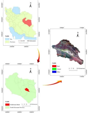
With an area of 242701.83ha, the Mokhtaran basin is located in the arid region of South Khorasan province. This is a sub-basin of the great Lut desert, with an arid climate and an average annual rainfall of 172mm. Its highest amount of rainfall (39mm) is in March and the minimum is in July and August. The average annual potential evapotranspiration, the average annual temperature and the average annual minimum temperature of this basin are 172mm, 14.3oC and 6.5oC, respectively. The aridity and water scarcity of this basin can be revealed by these mentioned characteristics. There are different types of agriculture from traditional to mechanized and modern systems in the study area. In terms of natural environment, there are various land surfaces from mountainous planes upstream to desert geomorphologic facies and sand dunes downstream (Figure 1).
2.2. Data set
Due to the need of high spectral, spatial, and temporal resolution in mapping and modeling projects, Landsat satellite data set present the most widely used data in applications for remote sensing (Hilker et al., 2009). In the present investigation, image classifications were carried out by Landsat 8 satellite data, recorded on May 30, 2015. The OLI (Operational Land Imager)
and the TIRS (Thermal Infrared Sensor) are two sensors of the Landsat 8 satellite. The satellite consists of 11 bands summarily shown in Table 1 (Roy etal., 2014). The sensitive sensor of OLI collects image data from the visible, near infrared and infrared bands with short wavelengths and the TIRS sensor is sensitive to two thermal infrared wavelength bands 11 and 12, in order to measure the temperature of earth's surface (Zanter, 2016).
Table 1. The Landsat 8 bands
Band description (30 m native resolution unless otherwise denoted) Wavelength (µm)
Band 1 — blue 0.43–0.45
Band 2 — blue 0.45–0.51
Band 3 — green 0.53–0.59
Band 4 — red 0.64–0.67
Band 5 — near infrared 0.85–0.88
Band 6 — shortwave infrared 1.57–1.65
Band 7 — shortwave infrared 2.11–2.29
Band 8 — panchromatic (15 m) 0.50–0.68
Band 9 — cirrus 1.36–1.38
Band 10 — thermal Infrared (100 m) 10.60–11.19
Band 11 — thermal Infrared (100 m) 11.50–12.51
In this study, the combination of bands 2, 3, 4, 5, 6, and 7 were used and the multi-spectral image was combined with panchromatic band 8 (PAN) to improve the resolution. There are a wide range of enhancement methods to make an image more analyzable in different applications. The Principal Components Analysis (PCA), used in the current study, is a common method applied for data compression. Nevertheless, in this work, PCA resolution merge (Chavez et al., 1991) was used to combine the system/map-corrected multispectral image with the PAN image to create a high-resolution color image. A dark subtraction technique was used for the correction of atmospheric scattering on the total scene (Chavez et al., 1988).
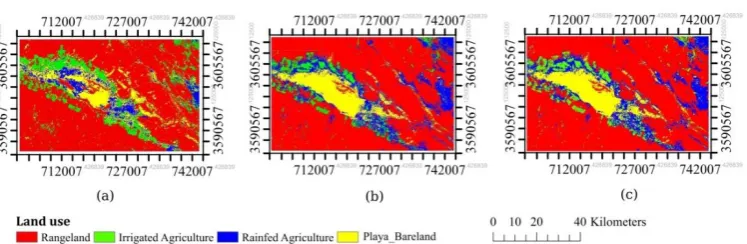
According to the 2015 land use map and field survey, four land use classes, irrigated agriculture, rangeland, rainfed agriculture, and playa bareland were considered and defined for classification.
2.3. Pixel-based classification with maximum likelihood method (MLC)
Supervised the MLC method is from the most broadly used methods of land cover classification (Dean and Smith, 2003; Richards and Jia, 2006). The algorithm is on the basis of the probability of belonging a pixel to a given class (Lillesand and Kiefer, 1994). In the original equation, it is assumed that this probability is the same for all classes and input bands are distributed, normally. MLC normally uses the following main equation:
(1)
gi(x)
= ln(ac) − [0.5 ln(|covc|)]
− [0.5(x − Mc)T(covC−1)((x − Mc))]
Where c denotes the desired class, x is the n-dimensional data. Where n stands for the number of bands, ac is the possibility of belonging a pixel to the class c and is assumed the same for all classes. Covc and Mc are determinant of covariance matrix and mean vector of class c, respectively. The ln stands for natural logarithm and T is the transposition function (Rees, 1999; Richards and Jia, 2006; Memarian et al., 2013).
2.4. Fuzzy Classification
In this study, a combination of the two methods of fuzzy and maximum likelihood were employed for land use classification. According to the theory of probability, if event A represents a set of elements in a large set (φ), then, the probability density function of A, i.e. P(A) is defined as follows (Branth and Mather, 2016; Akbarpour et al., 2006 ):
(2)
𝑃(𝐴) = ∫ 𝐻𝐴 .
𝜑
. (𝑆)
(membership grade equal to zero). If A is considered as a fuzzy event and a fuzzy subset of set φ, the probability density function of A will be equal to:
(3)
𝑃(𝐴) = ∫ 𝜇𝐴 𝐴
𝜑
. (𝑆)
μA is the membership function. The mean and variance of the fuzzy set A is defined below (Branth and Mather, 2016):
(4)
𝑉(𝐴) = 1 𝑃(𝐴)∫ 𝑆. 𝜇𝐴
𝐴
𝜑
. (𝑆)
(5)
𝛿2
𝐴= ∫(𝑆 − 𝑉𝐴)2. 𝐴
𝜑
𝑆. 𝜇𝐴
The defuzzification process, i.e. categorizing each pixel to a particular class, may be operated using the following equation (Akbarpour et al., 2006; Khan et al., 2012):
(6)
𝑇[𝐾] = ∑ ∑ ∑ 𝑊𝑖𝑗 𝐷𝑖𝑗𝑙[𝑘] 𝑛
𝑙=0 𝑆
𝑗=0 𝑆
𝑖=0
Where, 𝑖 stands for the kernel row profile, 𝑗 shows an index for the kernel column profile, 𝑆 is the kernel size (3, 5 or 7), 𝑙 is an index of fuzzy set layer, 𝑛 denotes the number of fuzzy layers, 𝑤 indicates the weight of window, 𝑘 is the class code, 𝐷[𝑘]is the value of the distance for class 𝑘, and 𝑇[𝐾]is the overall weighted distance of the window belonging to class k. The center pixel of each window will belong to a class with the maximum 𝑇[𝐾].
2.5. Object-based K-Nearest Neighbor Classifier (K-NN)
Object-based analysis is made up of two parts; the first part is a segmentation of the image and the second part shows a classification based on the characteristics of objects in spatial and spectral domains. The image can be divided into homogeneous, continuous, and interconnected objects in segmentation. In this paper, the desired objects were explored and extracted with a variety of images in the module ENVI FX. Edge segmentation algorithm describes the lines along the highest slope and detects the edges more effectively. Full Lambda Schedule merging approach (Liu et al., 2011) combines the adjacent segments to increase the merging level (ENVI Tutorial, 2015). In this study, a merge level of 50 was considered reasonable. Scale Level
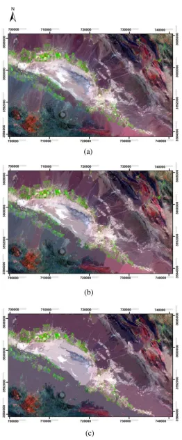
parameter (SL) is considered as a significant factor in analyzing images based on the object-based algorithm which determines the maximum allowed heterogeneity for the objects of an image (ENVI Guide, 2010; Memarian et al., 2013). In this paper, based on a visual examination and suggestions of previous articles (Wang et al., 2004; Yu et al., 2006; Mathieu et al., 2007; Memarian et al., 2013), three different SLs (10, 30, and 50) have been employed for image segmentation (Figure 2).
The K-NN method used in this work classifies the segments according to their proximity to the neighboring training districts. The K parameter represents the number of neighbors during classification. The perfect choice for K relies on selected data set and training data. After choosing the type of algorithm, the number of neighbors was determined which began from 3 and increased to 5 and 7. Combining the neighbor values with scale levels (10, 30, and 50), nine SL and NN combinations were obtained that were involved in the production of a classified map. Their results were compared by evaluating the accuracy of classification. These 9 combinations include SL10-NN3, SL10-NN5, SL10-NN7, SL30-NN3, SL30-NN5, SL30-NN7, SL50-NN3, SL50-NN5, and SL50-NN7.
2.6. Accuracy Assessment
Pontius (2000) presented some conceptual problems in the standard index of Kappa and applied some modifications on the index in order to correct its deficiencies. Standard Kappa and its variants are frequently complicated to compute, difficult to understand, and unhelpful to interpret. Pontius suggested alternative indices which are more appropriate, and which have a more simple computation approach. These indices concentrate on two components of disagreement between maps in terms of quantity as well as spatial allocation of the classes (Pontius and Millones, 2011). The disagreement parameters specify the difference between the observed and simulated maps (Pontius et al., 2008; Memarian
2.7. Disagreement Components
As shown in Table 2, 𝑗 represents the quantity of classifications as well as the number of strata in a common stratified sampling plan. With a range of 1 to 𝑗, the index 𝑖 shows each presented class in the comparison map. The quantity of the pixels in each layer is expressed by 𝑁𝑖. In the
comparison map (𝑖) and the reference map (𝑗), each recorded observation is constructed on its category. The quantities of these perceptions are summed as the recorded 𝑛𝑖𝑗 in row 𝑖 and column
𝑗 of the likelihood matrix. The ratio of the study zone (𝑝𝑖𝑗) from the simulated map and observed
map indexed Where, 𝑖 and 𝐽 can be estimated by the following equation (Pontius and Millones, 2011; Memarian et al., 2012; Memarian et al., 2013), respectively.
(7)
𝑝𝑖𝑗= ( 𝑛𝑖𝑗 ∑𝐽𝑗=1𝑛𝑖𝑗
) ( 𝑁𝑖 ∑𝐽𝑖=1𝑁𝑖
)
Quantity disagreement (qg) for an optional
class g is computed by Equation (8):
(8)
𝑞𝑔= |(∑ 𝑝𝑖𝑔 𝐽
𝑖=1
) − (∑ 𝑝𝑔𝑗 𝐽
𝑗=1
)|
Table 2. The scheme of estimated population matrix described by Pontius and Millones (2011) Reference
Comparison total
j=1 j=2 … j=J
C
o
m
p
ar
iso
n
i=1 P11 P12 P1J ∑ 𝑝1𝑗
𝐽
𝑗=1
i=2 P21 P22 P2J ∑ 𝑝2𝑗
𝐽
𝑗=1
…
i=J PJ1 PJ2 PJJ ∑ 𝑝𝐽𝑗
𝐽
𝑗=1
Reference total ∑ 𝑝𝑖1 𝐽
𝑖=1 ∑ 𝑝𝑖2 𝐽
𝑖=1 ∑ 𝑝𝑖𝐽
𝐽
𝑖=1 1
Overall quantity disagreement that contains all J classes is computed by equation (9)
(9)
𝑄𝐷 =∑ 𝑞𝑔
𝐽 𝑔=1
2
We estimate the allocation disagreement (ag)
for an optional class g with equation 10. The omission and commission of class g is shown respectively by the first and second quarrel within a minimum function.
(10)
𝑎𝑔= 2 min [(∑ 𝑝𝑖𝑔 𝐽
𝑖=1
) − 𝑝𝑔𝑔,(∑ 𝑝𝑔𝑗 𝐽
𝑗=1
) − 𝑝𝑔𝑔]
Total allocation disagreement is evaluated by equation (11):
(11)
𝐴𝐷 =∑ 𝑞𝑎𝑔
𝐽 𝑔=1
2
Agreement Proportion (𝐶) is computed by equation (12), as follows:
(12)
𝐶 = ∑ 𝑝𝑗𝑗 𝐽
𝑗=1
Total disagreement (𝐷 ), the entirety of the total 𝑄𝐷 and 𝐴𝐷, is measured as follows:
(13)
𝐷 = 1 − 𝐶 = 𝑄𝐷 + 𝐴𝐷
2.8. Pierce Skill Score
The class memberships of the validation pixels can be calculated using the skill score which represents the difference between calculated accuracy using the validation data and expected accuracy (Eastman, 2016). The determination of skill of threshold forecast begins with the creation of a contingency table of the form as shown below:
Table 3. The 2×2 Contingency Table
Observed
Yes No
Forecasted Yes a b
In regards to Table 3, the following points are: a) forecast-observation pairs named hits, b) occasions named false alarms, c) occasions named misses, d) occasions named correct rejection or correct negative. The Peirce skill score (PSS) is a skill measure that can be determined by equation (14):
(14)
𝑃𝑆𝑆 = 𝑎𝑑 − 𝑏𝑐 (𝑎 + 𝑐)(𝑏 + 𝑑)
= 𝐻 − 𝐹 Range: [−1 , 1]
According to equation (14), the PSS that is recognized as the true skill statistic is achieved with the difference between the hit rate and the false alarm rate, in which F represents a value of the rate at which false alarms occur:
(15)
Range:[0 ,1]
False Alarm Rate(F) = 𝑏 𝑎 + 𝑏
The hit rate is often called the “probability of detection” and measures how well observed cases are forecast.
(16)
Range:[0 ,1]
Hit Rate(𝐻) = 𝑎 𝑎 + 𝑐
If the value of PSS which ranges from -1 to 1 is greater than zero, the amount of hits surpasses the false alarms and the forecast has some skill (Stephenson, 2000; Wilks, 2011).
3. Results and Discussion
Figure 3 shows the maps that have been classified with maximum likelihood, fuzzy, and object-based algorithms. Table 4 shows the components of disagreement at the class and total landscape levels based on the algorithms MLC, Fuzzy-MLC, and object-based K-NN. The QD and AD measures all over the landscape using MLC which was determined to be 16.36% and 8.07%, respectively. In comparison to other
methods, MLC with larger QD and AD values, showed less accuracy than the other methods. However, there is an exception where the total AD of MLC is less than the SL10-NN3 object-based classification. The ratio of QD to Areal Proportion (AP) and AD to AP of each land use class presents a more suitable description for the relationship between each land acreage unit and the resulting error. According to Table 4, it could be explored that rainfed agriculture class produces the highest ratio of QD/AP and QD/AP, which represents the lowest quantitative accuracy and location accuracy of classified pixels.
The Fuzzy-MLC method yielded lower error in compare to the MLC
with
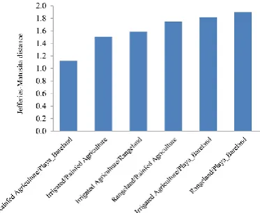
the QD and AD of 15.35% and 7.10%, respectively. On the other hand, it showed greater error in comparison with the K-NN classifier. As illustrated in Figure 4, the highest ratio of QD/AP and AD/AP could be found in the rainfed agriculture, in which both approaches, Fuzzy-MLC and MLC, showed the lowest accuracy. Among the object-based classifiers, SL30-NN3, with a QD of 4.19% and AD equal to 5.95%, showed the highest classification accuracy in a total landscape. Thus, in terms of classification accuracy, the best combination is obtained with SL30 and NN5. According to the results of the SL30-NN3 classifier, irrigated agriculture showed the highest participation in quantitative disagreement, as the QD/AP ratio with a value of 0.11 was greater than that ratio of the other land use classes. Rainfed agriculture with an AD/AP equal to 0.27 designated the highest allocation error (Figure 4). According to Figure 5, it can be seen that the rainfed agriculture and playa_bareland had the lowest spectral separability in the Jeffries–Matusita distance. Thus, the higher values of QDs and ADs can be expected for the rainfed agriculture and playa_bareland.Table 4. Accuracy evaluation of land use maps classified by different utilized approaches
Class MLC Fuzzy-MLC
QD (%) QD/AP AD (%) AD/AP QD (%) QD/AP AD (%) AD/AP
IrrigatedAgriculture 16.36 0.41 2.58 0.06 15.35 0.34 2.42 0.05
Rangeland 1.51 0.05 4.28 0.13 0.97 0.03 3.93 0.12
Rainfed Agriculture 11.96 0.95 7.29 0.58 11.45 0.94 6.82 0.56
Playa_Bareland 2.89 0.18 2.00 0.13 2.92 0.36 1.02 0.13
Total 16.36 8.07 15.35 7.10
Class
Object-based K-NN
SL10-NN3 SL10-NN5 SL10-NN7
QD
(%) QD/AP AD
(%) AD/AP
QD
(%) QD/AP AD
(%) AD/AP
QD
(%) QD/AP AD
(%) AD/AP IrrigatedAgriculture 1.50 0.04 5.62 0.14 3.97 0.10 2.94 0.07 3.61 0.09 3.00 0.08
Rangeland 1.77 0.06 4.89 0.15 2.96 0.09 1.23 0.04 2.26 0.07 1.61 0.05
Rainfed Agriculture 1.20 0.10 2.92 0.23 1.17 0.09 4.22 0.34 1.22 0.10 3.82 0.30
Playa_Bareland 0.94 0.06 6.95 0.44 2.18 0.14 4.63 0.29 2.57 0.16 3.97 0.25
Total 2.70 10.19 5.14 6.51 4.83 6.20
Class
Object-based K-NN
SL30-NN3 SL30-NN5 SL30-NN7
QD
(%) QD/AP AD
(%) AD/AP
QD
(%) QD/AP AD
(%) AD/AP
QD
(%) QD/AP AD
(%) AD/AP
IrrigatedAgriculture 4.19 0.11 3.00 0.08 4.82 0.12 2.07 0.05 5.82 0.15 1.65 0.04
Rangeland 2.48 0.08 1.62 0.05 3.24 0.10 1.33 0.04 3.52 0.11 1.09 0.03
Rainfed Agriculture 1.05 0.08 3.39 0.27 1.09 0.09 3.40 0.27 1.45 0.12 3.33 0.27
Playa_Bareland 0.67 0.04 3.89 0.24 0.49 0.03 4.70 0.30 0.85 0.05 4.06 0.26
Total 4.19 5.95 4.82 5.75 5.82 5.07
Class
Object-based K-NN
SL50-NN3 SL50-NN5 SL50-NN7
QD
(%) QD/AP AD
(%) AD/AP
QD
(%) QD/AP AD
(%) AD/AP
QD
(%) QD/AP AD
(%) AD/AP IrrigatedAgriculture 9.51 0.24 0.73 0.02 10.48 0.26 0.50 0.01 11.07 0.28 0.40 0.01
Rangeland 7.51 0.24 0.30 0.01 9.17 0.29 0.17 0.01 9.46 0.30 0.22 0.01
Rainfed Agriculture 1.75 0.14 3.47 0.28 1.03 0.08 3.34 0.27 1.03 0.08 3.42 0.27
Playa_Bareland 0.25 0.02 5.41 0.34 0.28 0.02 5.55 0.35 0.58 0.04 5.55 0.35
Fig. 4. The ratios related to each land use class: (a) QD/AP and (b) AD/AP
Fig. 5. Jeffries–Matusita distance for pair separation
According to Table 4, SL30-NN3 in comparison with MLC and Fuzzy-MLC reduced the quantity error by 12.16 (290%) and 11.16 (265%), respectively. Moreover, the total error is decreased by 14.28% and 12.3%. It is obvious that SL30-NN3 reduced the quantity error more than the Fuzzy-MLC in comparison to MLC.
Results of maximum likelihood classification reflect a generally higher incapability compared to the fuzzy-based image classification and object-based classification. Conclusively, we can establish that object-based method show more accuracy than pixel-based methods in the classification of remote sensing images. Gao and Mas (2008) provided a similar example in the use of pixel-based and object-based image analysis in classification of land use/cover. They employed satellite images with various spatial resolutions and compared the performance results of the object-based algorithm with the consequences of the classification based on pixels. Results confirmed a higher capability of the object-based method, in comparison to the pixel-based algorithms, for land use classification. However, an increase in the spatial resolution decreased the difference in the accuracy values between object-based and pixel-based methods.
In the current study, the fuzzy approach showed higher accuracy in comparison to the
maximum likelihood classification method. This proficiency was established by other research efforts. For instance, Zhang and Foody (2001) compared two fuzzy and artificial neural network approaches and introduced the fuzzy method as the best classification method for land use mapping. Akbarpour et al. )2006) used two maximum likelihood and fuzzy classifiers for land use mapping of the Kameh basin, Iran. The results indicated a higher robustness of the fuzzy method than the maximum likelihood approach.
Meymeh, Iran. They realized that the object-based classification was more robust compared to the pixel-based methods.
It has been established that the analysis of the traditional pixel-based image is restricted due to the following reasons: image pixels are not real geographical objects and the pixel topology is limited; the spatial photo-interpretive elements such as texture, context, and shape are principally ignored in pixel based image analysis; and, the enhanced implicit variability within high spatial resolution imagery complicates traditional pixel-based classifiers that leads to lower classification accuracies (Hay and Castilla, 2006; Gao and Mas, 2008).Unlike the pixel-based method, object-based image
analysis can be applied on homogeneous objects made by image segmentation and additional features can be employed in the classification. Since an object is a group of pixels, the object’s characteristics such as mean digital number value, standard deviation, band ratio, etc. can be computed; moreover, there are shape and texture features of the objects available which can be applied for differentiating the land cover classes with parallel spectral information (Table 6). Such extra information gives the object-based image analysis a potential to make land cover thematic maps with greater accuracies, compared to those created by conventional pixel-based technique (Gao and Mas, 2008).
Table 5. Pierce Skill Score for Boolean Case (PSS)
Classifier PSS
SL10-NN3 0.89
SL10-NN5 0.90
SL10-NN7 0.91
SL30-NN3 0.90
SL30-NN5 0.89
SL30-NN7 0.88
SL50-NN3 0.81
SL50-NN5 0.78
SL50-NN7 0.77
From the results, it is generally indicated that the object-based classification is more realistic and more detailed in providing a land use map compared to pixel-based classification. This finding is compatible with previous reports provided by Wang et al. (2004), Yan et al. (2006), Chen et al. (2009), and Myint et al. (2011). In spite of the higher capabilities of the object-based approach in image classification, the differences between the two types of algorithms at run time still remain a challenge, especially for large surface areas (Duro et al., 2012). The future development of object-based algorithms, in order to select the optimal segmentation parameters, will hopefully reduce the required time for the object-based image classification method, as shown by Costa et al. (2008) and Dragut et al. (2010). The investigation also indicates a better performance and higher capability of disagreement components in evaluating the accuracy of the classified maps confirmed by Pontius and Millones (2011), Memarian et al. (2012), and Memarian et al. (2013).
4. Conclusion
Results established that MLC compared to the K-NN classifiers had a greater quantity and
Table 6. Spatial, spectral, and textural features used in the object-based image categorization, (obtained from the SL30-NN3 classified image
CLASS_NAME Irrigated Agriculture Rangeland Rainfed Agriculture Playa_Bareland
FX_CONVEX 1.20 1.18 1.23 1.24
FX_ROUND 0.51 0.51 0.48 0.51
FX_ELONG 1.76 1.86 1.75 1.74
FX_RECT_FI 0.64 0.68 0.61 0.63
AVG_B1 13565.08 13198.12 15144.56 14272.70
STD_B1 442.50 318.10 384.51 488.44
AVG_B2 13071.33 12908.74 14609.38 13855.08
STD_B2 409.15 299.26 377.11 462.97
AVG_B3 11566.51 11453.96 12872.47 12241.00
STD_B3 353.73 245.76 316.86 386.45
AVG_B4 10317.13 10305.55 11179.12 10794.69
STD_B4 287.11 202.25 256.19 310.82
AVG_B5 9665.65 9733.33 10176.60 9980.98
STD_B5 259.43 188.11 229.41 276.98
AVG_B6 12210.79 11960.42 13975.30 12991.63
STD_B6 427.89 310.59 381.67 472.73
TXRAN_B1 1356.26 1095.65 1189.93 1454.60
TXRAN_B2 1232.59 1042.34 1143.07 1363.06
TXRAN_B3 1051.03 859.71 973.68 1147.28
TXRAN_B4 853.71 699.03 785.06 924.06
TXRAN_B5 774.14 641.57 702.46 826.14
TXRAN_B6 1272.49 1074.17 1160.51 1393.21
Notes: FX_RECT_FI: a shape measure that shows how well a rectangle describes the shape; AVG_B x: average value of pixels including the region in band x; STD_B x: standard deviation value of pixels including the region in band x; TXRAN: Average data range of pixels including the region inside the kernel.
Acknowledgments
The authors would like to acknowledge Semnan University for its valuable support throughout this research performance.
Confflict of Interest
The authors declare no conflict of interest in respect to the distribution of this original copy.
References
Akbarpour, A. A., M. B. Sharifi, H. Memarian, 2006. The Comparison of Fuzzy and Maximum Likelihood Methods in Preparing Land Use Layer Using ETM+ Data (Case Study: Kameh Watershed). Range and Desert Research, 22; 27–38.
Blaschke, T., S. Lang, E. Lorup, J. Strobl, P. Zeil, 2000. Object-Oriented Image Processing in an Integrated GIS/Remote Sensing Environment and Perspectives for Environmental Applications. Environmental Information for Planning, Politics and the Public 2; 555-570.
Blaschke, T., 2010. Object based Image analysis for Remote Sensing. ISPRS Journal of Photogrammetry and Remote Sensing, 65; 2-16.
http://dx.doi.org/10.1016/j.isprsjprs.2009.06.004. Bocco, M., G. Ovando, S. Sayago, E. Willington, 2007.
Neural Network Model for Land Cover Classification from Satellite Images. Agricultura Técnica, 67; 414– 421.
Baatz, M., A. Schape, 2000. Multiresolution Segmentation–an Optimization Approach for High Quality Multi-scale Image Segmentation. In: J. Strobl, T. Blaschke & G. Griesebner (eds.), Angewandte Geographische Informations verarbeitung XII, Wichmann Verlag, Heidelberg, pp. 12–23.
Brandt, T., P.M. Mather, 2016. 2nd ed., Classification Methods for Remotely Sensed Data. CRC press, Boca Raton, 376p.
Cohen, J., 1960. A coefficient of agreement for nominal scales. Educational and Psychological Measurement, 20; 37-46.
http://dx.doi.org/10.1177/001316446002000104. Campbell, N. A., 1984. Some aspects of allocation and
discrimination. In Multivariate Statistical Methods in Physical Anthropology. Springer, Dordrecht, p. 177– 192. https://doi.org/10.1007/978-94-009-6357-3_12. Chavez, P. S., 1988. An improved dark-object subtraction
Chavez, P., S. C. Sides, J. A. Anderson, 1991. Comparison of three different methods to merge multiresolution and multispectral data- landsat tm and spot panchromatic. Photogrammetric Engineering and Remote Sensing, 57; 295-303. Casals-Carrasco, P., S. Kubo, B. B. Madhavan, 2000.
Application of spectral mixture analysis for terrain evaluation studies. International Journal of Remote Sensing, 21; 3039-3055.
http://dx.doi.org/10.1080/01431160050144947. Costa, G. A. O. P., R. Q. Feitosa, T. B. Cazes, B. Feijó,
2008. Genetic Adaptation of Segmentation Parameters. Object-Based Image Analysis, Springer, Heidelberg, p. 679–695.
https://doi.org/10.1007/978-3-540-77058-9_37. Chen, M., W. Su, L. Li, C. Zhang, A. Yue, H. Li, 2009.
Comparison of pixel-based and object-oriented knowledge-based classification methods using SPOT5 imagery. WSEAS Transactions on Information Science and Applications, 6; 477-489. De Kok, R., T. Schneider, U. Ammer, 1999. Object-Based
Classification and Applications in the Alpine Forest Environment. International archives of photogrammetry and remote sensing, Valladolid, Spain. 32, part 7–4–3 Wg.
Drǎguţ, L., D. Tiede, S. R. Levick, 2010. ESP: A tool to estimate scale parameter for multiresolution image segmentation of remotely sensed data. International Journal of Geographical Information Science, 24; 859-871.
http://dx.doi.org/10.1080/13658810903174803. Dean, A. M., G. M. Smith, 2003. An evaluation of
per-parcel land cover mapping using maximum likelihood class probabilities. International Journal of Remote Sensing, 24; 2905-2920.
http://dx.doi.org/10.1080/01431160210155910. Dingle Robertson, L., D. J. King, 2011. Comparison of
pixel- and object-based classification in land cover change mapping. International Journal of Remote Sensing, 32; 1505-1529. http://dx.doi.org/ 10.1080/01431160903571791.
Dehvari, A., R. J. Heck, 2009. Comparison of object-based and pixel object-based infrared airborne image classification methods using DEM thematic layer. Geography and Regional Planning, 2; 86-96. Duro, D. C., S. E. Franklin, M. G. Dubé, 2012. A
comparison of pixel-based and object-based image analysis with selected machine learning algorithms for the classification of agricultural landscapes using SPOT-5 HRG imagery. Remote Sensing of Environment, 118; 259–272.
http://dx.doi.org/10.1016/j.rse.2011.11.020.
Exelis Visual Information Solutions Inc., 2015. Feature Extraction with Example-Based Classification Tutorial. In: Harris Geospatial Corporation.
Eastman, J.R., 2016. IDRISI Terrset Manual. Clark Labs-Clark University: Worcester, USA, 391p.
Foody, G. M., N. A. Campbell, N. M. Trodd, d T. F. Wood, 1992. Derivation and applications of probabilistic measures of class membership from the maximum-likelihood.
classification. Photogrammetric Engineering and Remote Sensing, 58; 1335-1341.
Flanders, D., M. Hall-Bayer, J. Pereverzoff, 2003. Preliminary evaluation of eCognition object-based software for cut block delineation and feature extraction. Canadian Journal of Remote Sensing, 29; 441–452. http://dx.doi.org/10.5589/m03-006.
Foody, M. G. 2004. Thematic Map Comparison. Photogrammetric Engineering & Remote Sensing, 70; 627-633.
https://doi.org/10.14358/PERS.70.5.627.
Fathizad, H., D. Tazeh, S. Kalantari, 2016. Assessment of pixel-based classification (ARTMAP Fuzzy Neural Networks and Decision Tree) and object-oriented methods for land use mapping (Case Study: Meymeh, Ilam Province). Arid Biome, 5; 69-82.
Gao, Y., J. F. Mas, 2008. A comparison of the performance of pixel-based and object-based classifications over images with various spatial resolutions. Earth Sciences, 2; 27-35.
Hay, G. J., G. Castilla, 2006. Object-Based Image Analysis: Strengths, Weaknesses, Opportunities and Threats (SWOT). The International Archives of the Photogrammetry, Remote Sensing and Spatial Information Sciences, Salzburg, July 4, p. 4–5. Hilker, T., Wulder, M.A., Coops, N.C., Linke, J.,
McDermid, G., Masek, J.G., Gao, F., White, J.C., 2009. A new data fusion model for high spatial-and temporal-resolution mapping of forest disturbance based on Landsat and MODIS. Remote Sensing of Environment, 113; 1613–1627.
https://doi.org/10.1016/j.rse.2009.03.007.
Khan, G. A., S. Khan, N. A. Zafar, S. Islam, F. Ahmad, M. ur Rehman, M. Ullah, 2012. A review of different approaches of land cover mapping, Life Science Journal, 9; 1023-1032.
Lillesand, M., W. R. Kiefer, 1994. Remote Sensing and Image Interpretation. 3th ed., John Wiley and Sons, New York, 750 p.
Lang, L., X. Wen, A. Gonzalez, D. Tan, J. Du, Y. Liang, D. Xiang, 2011. An object-oriented daytime land-fog-detection approach based on the mean-shift and full lambda-schedule algorithms using EOS/MODIS data. International Journal of Remote Sensing, 32; 4769-4785.
http://dx.doi.org/10.1080/01431161.2010.489067. Memarian, H., S. K. Balasundram, J. B. Talib, C. T. B.
Sung, A. M. Sood, K. Abbaspour, 2012. Validation of ca-markov for simulation of land use and cover change in the langat basin, malaysia. Geographic Information System, 4; 542-554. http://dx.doi.org/_ 10.4236/jgis.2012.46059.
Memarian, H., S. K. Balasundram, R. Khosla, 2013. Comparison Between Pixel-and Object-Based Image Classification of a Tropical Landscape Using Système Pour l’Observation de la Terre-5 Imagery. Applied Remote Sensing, 7; 073512-073512. http://dx.doi.org/10.1117/1.JRS.7.073512-073512. Myint, S. W., P. Gober, A. Brazel, S. Grossman-Clarke,
Q. Weng, 2011. Per-Pixel vs. object-based classification of urban land cover extraction using high spatial resolution imagery. Remote Sensing of Environment, 115; 1145-1161.
http://dx.doi.org/10.1016/j.rse.2010.12.017. Mathieu, R., J. Aryal, 2007. Object-based classification
of ikonos imagery for mapping large-scale vegetation communities in urban areas. Sensors, 7; 2860–2880. http://dx.doi.org/10.3390/s7112860.
Photogrammetric engineering and remote sensing, 66; 1011–1016.
Pontius, R. G., W. Boersma, J. C. Castella, K. Clarke, T. de Nijs, C. Dietzel, P. H. Verburg, 2008. Comparing the input, output, and validation maps for several models of land change. The Annals of Regional Science, 42; 11–37.
http://dx.doi.org/10.1007/s00168007-0138-2. Pontius, R. G., M. Millones, 2011. Death to Kappa: Birth
of Quantity Disagreement and Allocation
Disagreement for Accuracy
Assessment. International Journal of Remote Sensing, 32; 4407–4429.
http://dx.doi.org/10.1080/01431161.2011.552923 . Rees, G., 1999. The Remote Sensing Data Book.
Cambridge university press, Cambridge, 262 p. Roy, D. P., M. A. Wulder, T. R. Loveland, C. E.
Woodcock, R. G. Allen, M. C. Anderson, T. A. Scambos, 2014. Landsat-8: science and product vision for terrestrial global change research. Remote Sensing of Environment, 145; 154-172. https://doi.org/10.1016/j.rse.2014.02.001.
Richards, J. A., X. Jia, 2006. Remote Sensing Digital Image Analysis. 4th ed., Springer, Berlin, 439 p. https://doi.org/10.1007/3-540-29711-1 .
Stephenson, D. B., 2000. Use of the “Odds Ratio” for diagnosing forecast skill. Weather and Forecasting, 15; 221-232.
https://doi.org/10.1175/1520-0434(2000) 015%3C0221:UOTORF%3E2.0.CO;2.
Singh, A., 1986. Change detection in the tropical forest environment of northeastern india using landsat. In: Eden MJ, Parry JT (eds), Remote Sensing and Tropical Land Management. Wiley, London, p. 237– 254.
Wilks, D. S., 2011. Statistical Methods in the
Atmospheric Sciences. Academic press, Amsterdam, 704 p.
Wang, Z., W. Wei, S. Zhao, X. Chen, 2004. Object-oriented classification and application in land use classification using SPOT-5 PAN imagery. In Proceedings of the IEEE International Geoscience and Remote Sensing Symposium, IGARSS ’04, Anchorage, Sept. 20–24, p. 3158–3160. https://doi.org/10.1109/IGARSS.2004.1370370. Wang, F., 1990. Improving remote sensing image
analysis through fuzzy information representation. Photogrammetric Engineering and Remote Sensing, 56; 1163–1169.
Yu, Q., P. Gong, N. Clinton, G. Biging, M. Kelly, D. Schirokauer, 2006. Object-based detailed vegetation classification with airborne high spatial resolution remote sensing imagery. Photogrammetric Engineering & Remote Sensing, 72; 799-811. https://doi.org/10.14358/PERS.72.7.799.
Yan, G., J. F. Mas, B. H. P. Maathuis, Z. Xiangmin, P. M. Van Dijk. 2006. Comparison of pixel-based and object-oriented image classification approaches-a case study in a coal fire area, Wuda, Inner Mongolia, China. International Journal of Remote Sensing, 27; 4039-4055.
https://doi.org/10.1080/01431160600702632. Zhang, J., G. M. Foody. 2001. Fully-fuzzy supervised
classification of sub- urban land cover from remotely sensed imagery: statistical and artificial neural network approaches. International Journal of Remote Sensing, 22; 615–628.