Max Planck Institute for Demographic Research Konrad-Zuse Str. 1, D-18057 Rostock·GERMANY www.demographic-research.org
DEMOGRAPHIC RESEARCH
VOLUME 22, ARTICLE 19, PAGES 549-578
PUBLISHED 07 APRIL 2010
http://www.demographic-research.org/Volumes/Vol22/19/ DOI: 10.4054/DemRes.2010.22.19
Research Article
Women’s wages and childbearing decisions:
Evidence from Italy
Concetta Rondinelli
Arnstein Aassve
Francesco C. Billari
c
°2010 Concetta Rondinelli et al.
2 Wage and childbearing decisions 551
2.1 Previous literature 551
2.2 The Italian setting 553
3 Data and methods 555
3.1 The Survey of Households’ Income and Wealth (BOI-SHIW) 556 3.2 The Italian Labour Force Survey (ISTAT-LFS) 556
3.3 Descriptive statistics and methods 557
4 Empirical results 559
4.1 First birth 560
4.2 Second and third birth 565
5 Summary and concluding remarks 568
6 Acknowledgements 569
References 570
Women’s wages and childbearing decisions: Evidence from Italy
Concetta Rondinelli1
Arnstein Aassve2
Francesco C. Billari3
Abstract
During the early 1990s, Italy became one of the first countries to reach lowest-low fer-tility. This was also a period in which women’s education and labour force participation increased. We analyze the role of women’s (potential) wages on their fertility decisions by making use of two different surveys. This enables us to apply discrete-time duration models. For first births, we find evidence of non-proportional hazards and of some “re-cuperation” effects; for second and third births, instead, wage exhibits small intensity although there is a clear division between Northern and Southern Italian regions.
1Bank of Italy, Economic Outlook and Monetary Policy Department, via Nazionale, 91, 00184 Roma, Italy.
E-mail: [email protected]. Corresponding author.
2Department of Decision Sciences and “Carlo F. Dondena” Centre for Research on Social Dynamics, Bocconi
University, Milan, Italy. E-mail: [email protected].
3Department of Decision Sciences, Innocenzo Gasparini Institute for Economic Research and “Carlo
1. Introduction
During the early 1990s, Italy became one of the first countries to reach lowest-low fertility, i.e. a Total Fertility Rate (TFR) below 1.3. Whereas the reasons behind the Italian fertility decline are many, a prominent explanation suggests that it has been driven by increasing opportunity costs. Certainly, the strong fertility decline during the nineties was followed by a significant increase of education and labour force participation among women. Given this setting it is of interest to establish the extent to which women’s wages are linked to their fertility decisions. As a result we analyze fertility behavior of Italian women during the period 1983 to 2003. We pay particular attention to the role of potential incomes (or predicted wages), which in turn depend directly on women’s educational attainment, and therefore their opportunity cost, and we investigate how this affects their childbearing decisions.
So far, research on this issue in Italy has been hampered by lack of data sources that contain information on both fertility behavior and women’s income or earnings. We over-come this problem by combining two different data sets. Data from the Italian Institute of Statistics Labour Force Survey of 2003 (ISTAT-LFS hereafter) are used to reconstruct women’s fertility histories. Potential wages (i.e. hourly labour income) are derived from the income and earnings data from the Bank of Italy’s Survey on Household Income and Wealth (BOI-SHIW). Data from the BOI-SHIW are used to predict women’s potential wage, which is then introduced as an explanatory variable in discrete time hazard regres-sion models for first, second, and third births.
Our analysis includes women aged between 15 and 40 years in 2003. Their predicted wages depend on a range of background variables, including their educational attainment. As such the predicted wages reflect their potential wage, which in turn is a measure of their socio-economic characteristics. Our interest lies in assessing the extent to which socio-economic characteristics, expressed through predicted wages, may play a key role in the postponement of motherhood in Italy and their impact in the transition to first, second and third birth. In particular, we assess whether potential wages are the only determinants in these transitions, or whether other socio-cultural factors may be in play for delayed motherhood and second and third birth decisions.
2. Wage and childbearing decisions
2.1 Previous literature
It is useful to start from an economic perspective when considering the role of wages and income on fertility. Becker (1960) argues that there should be a positive correlation between the number of children and the household income. Highly educated mothers, however, tend to substitute child quality for number of children (see Becker and Lewis (1973)). Since both production and rearing of children are time intensive, an increase in wage rates induces a negative substitution effect on the demand for children (see for instance Becker (1965); Mincer (1963)). To this extent, theoretical research on fertility (such as Hotz, Klerman, and Willis (1997); Becker (1981); Willis (1973)) shows that women’s income is negatively associated with childbearing as a higher income implies higher opportunity cost of children. In other words, with high earnings, it becomes more expensive for her to take time away from work to rear children. In general, the opposing income effect is unlikely to outweigh the negative substitution effect. Overall, therefore, we would expect the effect from women’s wages to be negative. For men, in contrast, the income effect tends to dominate since they spend less time on rearing children, though the magnitude of these effects will vary across countries and birth parity (Butz and Ward 1979; Willis 1973).
In recent years research has shifted towards investigating the timing of births rather than completed fertility (see for instance Heckman and Walker (1990a)). In these studies, hazard rate models are used to empirically analyze the timing and spacing of births. Most of the studies show that, compared to women with low opportunity costs, women with high wages (i.e. high opportunity cost of having children) have births later. However, a source of potential conflicting patterns is present among high-earning postponers. Higher incomes can mean both higher opportunity costs and a better ability to pay for high cost private child-care, as previously discussed. There is also ample evidence to suggest that the presence of children has a significant negative impact on the woman employment probability (see Mroz (1987); Heckman and Macurdy (1980)). Women with high earnings stay longer in education, and possibly in the labour market, before they have the first child. For this reason, return to work might be a more affordable option for high-earning women, while others are more likely to give up. As Pronzato (2009) shows this can be due to the lack of protected leave, low childcare availability and attitudes on gender roles and family-work orientation.
A prominent part of the existing literature argues that women’s responsibility for child-rearing may reduce her time in paid work. Joshi (1990), for instance, analyzes how work patterns can be different, in terms of switching from full time to part time work or not employed, by comparing mothers with childless women. The causal direction is explained through the impact of children on the women’s job market opportunities and their level of income. Miller (2010) and Waldfogel (1998) offer similar perspectives.
Likewise, the decision to enter parenthood has important time dimensions to it. A couple may want to pay attention to the cost of having childrenearly, comparing it with the cost of having themlater. In such a way, the optimal age of having the first birth can be seen as a trade-off between investment in human capital and career planning (see Gustafsson (2001)). As emphasized by Cigno and Ermisch (1989), Cigno (1991) and Gustafsson and Wetzels (2000), it is important to take into account possible consequences to lifetime earnings given different scenarios of birth timing and spacing. In light of this it may be optimal for many women to delay motherhood until the opportunity cost of child-care (with respect to her child-career) has decreased, which implies completion of education and getting a foothold in the labour market, before entering motherhood.
mother-hood, because they are in a position to negotiate a family-friendly work environment with flexible work schedules. Similar evidence is shown for the British case (Kneale and Joshi 2008).
2.2 The Italian setting
Figure 1 provides stylized facts of fertility in Italy. Two prevalent trends are depicted for the last two decades in Italy: a decline in total fertility and a steady increase in women’s educational attainment, together with higher female employment rates (see also Figure 2). Using a sensitivity analysis, Rindfuss, Guzzo, and Morgan (2003) showed that a 1% increase in female labour force participation was associated with a 3.15% decline in Total Fertility Rate. During the same period, the mean age of onset of motherhood increased from 25 years in 1980 to almost 27 in 1990, reaching a level of 28 years in 1995 and 28.7 in 1997 (Figure 2).
Figure 1: Education, TFR and female participation rates in Italy (1992-2004)
Notes: Fertility rates: 1998 and 1999 are provisional values and 2000, 2001, 2002 are estimated values. Education is the percentage of the female population aged 20 to 24 having completed at least upper secondary education. The female employment rate is calculated by dividing the number of women aged 15 to 64 in em-ployment by the total female population of the same age group.
Figure 2: Mean age at first birth, at childbirth and TFR in Italy (1960-2000)
Notes: Mean age of women at childbearing is the mean age of women when their children are born. For a given calendar year, the mean age of women at childbearing can be calculated using the fertility rates by age (in general, the reproductive period is between 15 and 49 years of age).
Source: Council of Europe (2001).
As Kohler, Billari, and Ortega (2002) point out, Italy was, together with Spain, the first country to reach the threshold of so-called lowest-low fertility, i.e., below 1.3 children per woman. It is well established that the emergence of the lowest-low fertility in Southern Europe is not connected to any steep increase in childlessness (Billari and Kohler 2004). Available parity-specific data on fertility show that most of the fertility decline in Italy during the last twenty years is due to a decreasing progression to the second, third and subsequent children. As a consequence, the probability of having a first child has not changed in spite of the tremendous economic and social changes of the Italian country during that period (see Dalla Zuanna 2004). Moreover, the personal ideal family size for around 60% of Italian women aged 20-34 years is two children; while one quarter has a preference for large families (Goldstein, Lutz, and Testa 2003).
third birth (i.e., women who stopped at two children), economic reasons were cited as important for women who experienced a worsening of their financial situation after the birth of the first and second child. Many women argued that monetary transfers for the first three years after the birth of a third child, or a lower but longer financial incentive, could have changed their decision to stop at parity two (De Santis and Breschi 2003). Although being possibly biased as an ex-post motivation, this role of economic factors is specific for third birth.
3. Data and methods
Micro evidence on the relationship between the timing and the spacing of births has been scarce for the Italian case, the main reason being a lack of data sources provided with wage and income information linked with women’s fertility histories, where the latter has sufficient sample size. The data requirement for estimating the impact of wage on the timing of births is demanding: we need panel data with a long time dimension or retrospective data on the complete employment and fertility histories. Usually, and this is our case, a researcher has available only cross section data or panel data with a short time dimension. Fertility histories may be reconstructed on the basis of the age of the children in the household but the complete labour market history of the women in the household will be more difficult or even impossible to reconstruct. This is because one observes, for each household, the number of children and the employment status of the women in the household only at the time of the interview.
Unfortunately none of the currently available Italian data sets contain all the required information. The BOI-SHIW provides detailed information on employment and income of family members, labour market activities, payment instruments and forms of savings, socio-demographic characteristics of the household. However, the sample size is too small to conduct fertility analysis, particularly for third births. The ISTAT-LFS, 2003, contains detailed information on the family structure, labour market, work experience, part time and full time employment. The main drawback of this survey is that it does not collect information on household earnings and income. The sample size is however large and suitable for fertility analysis.
3.1 The Survey of Households’ Income and Wealth (BOI-SHIW)
The BOI-SHIW started in 1964 and it is provided with an annual and historical version. Because a long time span is analyzed, this paper uses the historical version of the sur-vey which is the main source of information on Italian household savings and wealth. The survey collects information on more than 22,000 individuals per year (around 8,000 households) with 13,500 individuals receiving an income. From the survey we have infor-mation on payroll employees, members of professions, family business and pensioners. Respondents report their annual wage (both if they are part and full time workers), the number of months and hours worked on average per week, so that we can construct an hourly wage measure independent from the opportunity cost of the woman dividing the annual net wages by the annual working hours.
The survey is provided with net wages, excluding tax and social security contribu-tion, but including month salary (“13 month” and “14 month” salary), bonuses or special allowances (family allowances, productivity bonuses, sales commissions, etc.).
Our unit of analysis is the woman. We only consider households in which it is possible to link every woman with their co-residing children. In total this produces a sample of 20,003 individuals in 2002 with 4,749 women in their childbearing stage. In other words, we consider women aged less than 40 years, who are not pensioners and not studying.
3.2 The Italian Labour Force Survey (ISTAT-LFS)
The ISTAT-LFS, implemented since 1959, has become a continuous survey in 2005. It was a quarterly survey up to 2004; for each year four waves are carried out. The survey collects information on more than 300,000 households, representing around 800,000 indi-viduals (1.4% of the total national population) distributed over 1,351 municipalities (out of 8,100). It assesses the state of the Italian labour market, supply side only. The sample design is a two stage rotating sample design with stratification of the primary units (mu-nicipalities). Each household is included first in two waves, then left out for two waves and then included in another two waves. The ISTAT-LFS offers different sections dealing with demographic characteristics of the households, present job (with all the information taken from the month before the interview), job experience, looking for a job, and re-lationship with public employment centers. However, there are no retrospective fertility histories available. Instead we know the number and ages of children living in the house-holds in which the woman is either the household head or the spouse of the household head.
the time of interview. Thus, we are able to reconstruct retrospective fertility histories for each woman back to 1983. We make the assumption the woman had a “regular” schooling career, as the dataset is provided to with the maximum level of education and the year this was achieved. It is reasonable assume that a woman drops out when she spends more than a “regular time” in an educational level. We also assume that the women in the dataset had no geographical mobility, a plausible assumption as the women’s internal migration was almost stable in the years 1988-2003 and attained 2% on average per year (Istat, General Population Register).
The sample includes a small number of adopted children or stepchildren, but we ex-clude any offspring who might have died or moved away. In Italy, mortality at adult age is low, children of divorced parents are almost exclusively living with their mothers, and a very low proportion of young individuals leave the parental household before the age of 23 (Aassve et al. 2002). Nevertheless, in order to ensure that the recorded children are the only ones of the mother, we limit the analysis to only include women who are aged 40 or less in 2003. Given that the mean age of leaving home is rather high in Italy (Aassve et al. 2002) this selection does not reduce the sample by much. We also exclude households in which we were unable to link children with mothers (i.e. male head of the household with no wife and all single men). In this way we end up with a sample of 34,129 women. In total, the fraction of women that can be matched with their co-residing children is 95%. Unfortunately, we are not able to use information of husbands since we only know the marital status of women at the time of interview. This problem also applies to widows, in that we do not know when the husband died.
3.3 Descriptive statistics and methods
Our methodological strategy can be summarized in three steps. First, using the historical version of the BOI-SHIW data, we estimate separate wage equations for the years 1991, 1993, 1995, 1998, 2000, 2002, assuming that for the period 1983-1991 wages evolved as they did in 1991. For the missing years, mean wages are interpolated from the adjacent years. Second, we match predicted wages onto the ISTAT-LFS data using common char-acteristics of women in both data sets. Third, we create three sub-samples consisting of women being at risk of the first, second and third birth.
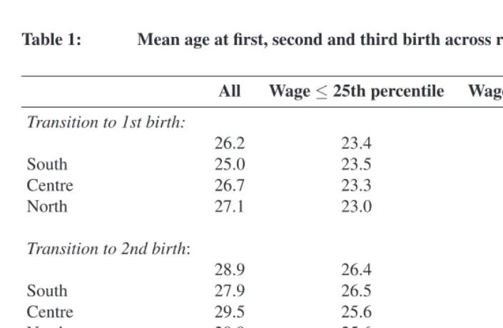
The details of estimation of wage equations is given in the appendix. The discussion of the relevant ISTAT-LFS descriptive statistics, using wages predicted from the BOI-SHIW, is reported in Table 1. We are assuming that a woman who is relatively poor in her 20s need not to be so in her 40s.
background, the regions are stratified into North, Centre and South. While poor women in the North (where poor means an hourly wage lower than the 25th percentile of the wage distribution for the whole country) start to have children early, women in the South tend to delay motherhood until they are 23.5. Transition to second (and respectively third) birth takes place on average two years after the first (second) child is born. Low (high) wage mothers living in the North tend to concentrate their fertility history in a shorter (longer) time span: they start at 23.0 (31.2) and end it after 4 (2) years, conditional on reaching the threshold of the 3rd birth.
Table 1: Mean age at first, second and third birth across regions and wage
All Wage≤25th percentile Wage≥75th percentile Transition to 1st birth:
26.2 23.4 31.3
South 25.0 23.5 31.5
Centre 26.7 23.3 31.9
North 27.1 23.0 31.2
Transition to 2nd birth:
28.9 26.4 31.7
South 27.9 26.5 31.5
Centre 29.5 25.6 32.7
North 29.9 25.6 31.5
Transition to 3rd birth:
30.8 29.1 32.9
South 30.4 29.2 33.6
Centre 31.3 27.8 33.4
North 31.4 26.7 32.7
Notes: The percentiles refer to the distribution of predicted hourly wage from the estimated wage equation as reported in the appendix. The means are for closed birth interval only (computed only for women experiencing a birth); women are classified according to the wage rate they had at birth. The 20 Italian regions are classified according to the following: Piemonte, Valle d’Aosta, Lombardia, Liguria, Trentino, Veneto, Friuli Venezia Giulia, Emilia Romagna belong to the North. Toscana, Umbria, Marche, Lazio are considered Central Regions. Abruzzi, Molise, Campania, Puglia, Basilicata, Calabria, Sicilia, Sardegna belong to the South.
The estimation of the impact of predicted and time-varying wage ωitˆ on fertility is implemented through a set of discrete time event models. Consider a series ofP predic-torsX1ij, X2ij, ..., XP ij and letxpij denote individuali’s values for thep-th predictor in timej. The hazard function is defined as:
h(tij) =P r[Ti=j|Ti≥jandX1ij =x1ij, X2ij =x2ij, ..., XP ij =xP ij] (1)
that is, the population value of discrete-time hazard for personiin time periodj is the probability that he/she will experience the target event in that time period,conditionalon no prior event occurrenceandhis or her particular values for thePpredictors in that time period (Jenkins 1995).
We estimate a variety of single spell discrete time duration models (Singer and Willett 2003) where the baseline hazard for the transition to first birth is a function of the age of the woman while the one for the transition to second (third) birth is a function of the spell, duration since first (second) birth. In order to asses the impact of predicted wage on fertility, different specifications of the model are offered: we start from a simple one controlling for wage and its square and extend it to allow for some interaction between covariates, capturing both duration and cultural/institutional effects.
The omission of relevant information for the husband could cause a serious bias in our model, as fertility decisions are expected to depend on the income level of the household. It has been proved that the omission of unobserved heterogeneity in single spell discrete time duration models causes a rescaling of all coefficients (Nicoletti and Rondinelli 2010). It has also been shown that the rescaling factor is close to one when using time varying coefficients. Given that wage is a time varying regressor the omission of the unobserved heterogeneity do not cause any relevant bias in the estimated parameter.
In all our discrete time duration models (estimated from ISTAT-LFS), wages are pre-dicted from BOI-SHIW. The standard errors are consequently corrected for the fact that we use generated regressors in the fertility equation (see Pagan (1984); Arellano and Meghir (1992)). To do so we use the bootstrap method with 300 replications and ob-servations clustered at the woman level. Any further increase in replications does not significantly affect the estimated standard errors.
4. Empirical results
4.1 First birth
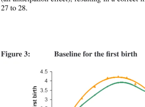
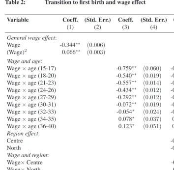
As expected, the baseline hazard for first births depicts an inverse U-shape. The effect of wages is approximated by a second order polynomial, which simply means that we include wages and its squared term in the regression. Column (1) of Table 2 shows that the general effect of women’s wage is negative: the higher the wage, the lower is the risk of entering motherhood (-0.344). The effect of wage is, however, nonlinear which is confirmed by the positive coefficient associated with the square term. Controlling for wage and its squared term only, the maximum of the parabola ranges between 30 and 31 as depicted in Figure 3, meaning that the mean age at first birth is between 30 and 31 years of age. This effect is, however, overestimated. In 1997, for example, the average age at first birth was 28.7 (see Council of Europe (2001)). As shown in Figure 3, once we control for interactions between age and wage, the baseline hazard is shifted to the left (an anticipation effect), resulting in a correct mean age for the first birth being between 27 to 28.
Figure 3: Baseline for the first birth
Table 2: Transition to first birth and wage effect
Variable Coeff. (Std. Err.) Coeff. (Std. Err.) Coeff. (Std. Err.)
(1) (2) (3) (4) (5) (6)
General wage effect:
Wage -0.344∗∗ (0.006)
(Wage)2 0.066∗∗ (0.003)
Wage and age:
Wage×age (15-17) -0.759∗∗ (0.060) -0.688∗∗ (0.062)
Wage×age (18-20) -0.540∗∗ (0.019) -0.475∗∗ (0.019)
Wage×age (21-23) -0.557∗∗ (0.014) -0.492∗∗ (0.015)
Wage×age (24-26) -0.434∗∗ (0.012) -0.371∗∗ (0.015)
Wage×age (27-29) -0.292∗∗ (0.012) -0.236∗∗ (0.016)
Wage×age (30-31) -0.072∗∗ (0.019) -0.023 (0.021)
Wage×age (32-33) -0.054∗ (0.024) -0.004 (0.027)
Wage×age (34-35) 0.078∗ (0.037) 0.125∗∗ (0.040)
Wage×age (36-40) 0.123∗ (0.051) 0.172∗∗ (0.052)
Region effect:
Centre -0.206∗∗ (0.023)
North -0.242∗∗ (0.020)
Wage and region:
Wage×Centre -0.040∗ (0.019)
Wage×North 0.008 (0.016)
Constant -5.735∗∗ (0.052) -6.132∗∗ (0.108) -5.935∗∗ (0.112)
No. of observations 425,014 425,014 425,014
No. of women 34,129 34,129 34,129
No. of spells 25,233 25,233 25,233
PseudoR2 0.086 0.090 0.091
Log-L -87524.64 -87159.352 -87064.898
Notes: Discrete-time logit hazard regressions. Baseline (i.e. age coefficient) not reported. Reference category for region is South. Bootstrapped standard errors in parentheses. Standard errors are computed using 300 bootstrap samples.
In columns (3) and (5) of Table 2, we report the estimated coefficients for women being at risk of the first birth where wage has been stratified by age and interacted with region. This allows us to understand how wage impacts on first birth after controlling for age and cultural or institutional effects. Column (3) of Table 2 shows that wage has a strong negative effect on the risk of the first birth for young women, the effect becoming closer to zero at the age of 34-35. Women with high wages have a higher likelihood of postponing motherhood which is confirmed by the importance of wages in driving the onset of motherhood. When controlling for regions (column (5) of Table 2), we mostly find the same negative pattern for younger women but the turning point is now between 32-33 years. After 34 years, increasing wage by one unit increases the likelihood to experience motherhood. Women in Central and Northern Italy are less at risk of first birth when compared with women in the South. However, when controlling for cultural and institutional effects (Wage and region effect of Table 2), high wage Central women are less likely to become mothers for the first time compared to the Southern one.
In order to better understand how different wage levels affect the timing of first birth, we simulate the hazard paths for a low and high wage woman. We choose two extreme situations. A low (high) wage woman is assigned a wage set equal to the 10th (90th) percentile of the hourly wage distribution. Both paths are plotted together with the hazard of the median wage woman in Figure 4. The Figure shows a non proportional hazard: low wage women are at a higher risk of experiencing the first birth when they are very young, reaching the maximum level when they are aged between 25 and 30 years of age. High wage women tend to delay, maximizing the likelihood for the first birth when they are 30 or older. The median wage woman has, not unexpectedly, an intermediate position. When the three paths cross (at age 32) low, median and high wage women experience similar risks though with the difference that a low wage woman has already reached her maximum, a median woman is at the maximum risk level and the high wage woman is yet to reach it.
the 75th percentile. The same is true if low wage women are defined according to the 10th percentile. We find that higher wages have their primary effect on postponement of first birth so that when wages are higher, pregnancy tends to be concentrated in a shorter span of the life cycle. This is in line with the opportunity cost theory (see Heckman and Walker (1990a)): few employed mothers would quit their job to have children if an exit from the labour market could seriously damage their future labour market prospects (Boix 1997). This effect would be more important the greater the uncertainty in the labour market or the higher the unemployment rate. This is one of the reasons why Central and Northern regions exhibit negative estimated coefficients for the risk of the first birth when compared to the South, where there is higher labour market uncertainty. In the Italian setting, characterized by an imperfect labour market (protecting those who are in, penalizing those who are out), starting late or discouraging a career can be very costly in terms of earnings so that it makes a lot of difference whether the woman is or is not employed, or a least has, or has never, been employed.
Figure 4: Timing of first birth for a low and high wage woman
Figure 5: Predicted survival curves. Postponement and recuperation effect
Notes: Median predicted survival per ages across wages (25th, 75th, 90th percentile). The proportion of women childless is estimated from Table 2, column (3). Recuperation effect is the vertical distance between the pre-dicted survival curves.
Another argument which is consistent with the negative interaction between wage and region is that, presumably, mothers with higher career prospects decide to postpone ma-ternity until they obtain a more stable labour market situation (e.g. getting a permanent contract, see De La Rica and Iza (2005) for an explanation for the Spanish case). Unfor-tunately, our data reconstruction of women’s job history makes it difficult to verify this hypothesis. However, it seems there is no institutional or cultural effect driving the first birth decision. If this was the case, we should have found a positive coefficient for the interaction of wage with North where a more efficient child care system is set up in order to help working mothers to reconcile job and family decisions.
4.2 Second and third birth
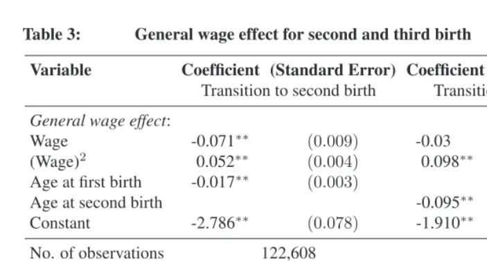
The fertility hazard is modeled in such a way that a woman becomes at risk of a second birth once she experienced the first; similarly, she becomes at risk of the third once she has experienced the second. A trivial consequence of this obvious fact (yet important for completed fertility) is that the age at first birth determines the age of becoming at risk of a second birth. However a delay in the first birth does not necessarily imply lower completed fertility as a woman may have an incentive to accelerate the second and third birth to achieve her desired fertility level. Our estimates in Table 3 prove that the higher the age of first birth, the less is the risk of second birth (-0.017).
Table 3: General wage effect for second and third birth
Variable Coefficient (Standard Error) Coefficient (Standard Error)
Transition to second birth Transition to third birth
General wage effect:
Wage -0.071∗∗ (0.009) -0.03 (0.018)
(Wage)2 0.052∗∗ (0.004) 0.098∗∗ (0.011)
Age at first birth -0.017∗∗ (0.003)
Age at second birth -0.095∗∗ (0.006)
Constant -2.786∗∗ (0.078) -1.910∗∗ (1.900)
No. of observations 122,608 83,949
No. of women 25,227 14,483
No. of spells 14,309 2,503
PseudoR2 0.440 0.024
Log-L -42221.856 -10989.240
Notes: Discrete-time logit hazard regressions for second and third birth. Baseline not reported. The number of women at risk of a second birth differs from the number of spells reported in Table 2 because women having twins as first births are not in the risk set of second birth as they are at risk of a third birth. Bootstrapped standard errors in parentheses. Standard errors are computed using 300 bootstrap samples.
†p <0.1;∗p <0.05;∗∗p <0.01.
Table 4: Wage and region effect for the transition to second and third birth
Variable Coefficient (Standard Error) Coefficient (Standard Error)
(1) (2) (3) (4)
Transition to second birth Transition to third birth
Age at first birth -0.026∗∗ (0.003)
Age at second birth -0.101∗∗ (0.006)
Wage and duration:
Wage×dur (1/2) -0.050† (0.029) -0.399 (5.588)
Wage×dur (3/4) 0.088∗∗ (0.016) -0.090 (0.073)
Wage×dur (5/6) -0.049∗∗ (0.018) 0.058 (0.048)
Wage×dur (7/9) -0.135∗∗ (0.024) -0.069† (0.042)
Wage×dur (10/13) -0.124∗∗ (0.041)
Wage×dur (10/14) -0.166∗∗ (0.045)
Wage×dur (14/25) 0.103 (0.079)
Wage×dur (15/24) -0.360∗∗ (0.085)
Region effects:
Centre -0.455∗∗ (0.030) -0.270∗∗ (0.084)
North -0.444∗∗ (0.025) -0.119† (0.066)
Wage and region:
Wage×Centre 0.003 (0.030) 0.166∗ (0.080)
Wage×North 0.116∗∗ (0.021) 0.181∗∗ (0.054)
Constant -2.258∗∗ (0.080) -1.679∗∗ (13.730)
No. of observations 122,608 83,949
No. of women 25,227 14,483
No. of spells 14,309 2,503
PseudoR2 0.050 0.024
Log-L -41986.374 -10987.727
Notes: Discrete-time logit hazard regressions for the transition to second and third birth. Baseline not reported. Reference category for Region is South. The number of women at risk of third birth differs from the number of spells reported for the transition to second birth because women having twins as second births are not in the risk set of third birth. Bootstrapped standard errors in parentheses. Standard errors are computed using 300 bootstrap samples.
Table 4 shows that women living in the Centre and North are less likely to experience a second or third birth compared to the South. But Table 4 also reveals a clear institutional or cultural effect underlined by the interaction of wage and region. An additional unit of wage for Northern women increases her risk to have a second or third birth. One might argue that this reflects confidence in the child-care system among working mothers living in the North and Centre (see Del Boca, Locatelli, and Vuri (2005) for a complete explanation). In Southern Italy, crêches are not widespread and working mothers tend to prefer informal child care, i.e. baby-sitters and grandmothers living nearby. When any of these two conditions is not satisfied, having another child means additional costs in terms of searching for childminders. The decision to have a second or third birth, even if in presence of higher wage, is therefore not straightforward (see also Diprete et al. (2003)). The situation is different in the North, where the large presence of public and private services offers a more reliable child-care system that also facilitates child-care even when children are very young (Del Boca, Locatelli, and Vuri 2005). We could also think there might be a selection effect at work. Only a few high wage women in the North have two children: if they are selected to for high fertility preferences, they tend to have a third child (see Kravdal (2001) for a different setting).
5. Summary and concluding remarks
The aim of this paper is to find an empirical connection between women’s potential wages and both the delay in motherhood and the transition to second and third birth in Italy.
Using two different data sets, we estimate the effect of predicted wages on the post-ponement of motherhood. First, a wage equation including detailed controls for women’s educational attainment is estimated using a Tobit model. Second, we use the predicted wage as a regressor in discrete time hazard models for the transition to first, second and third births. We find that the wage effect is negatively correlated with having children. The magnitude, however, varies according to the birth order. Wage has a strong negative effect in the timing of first birth. Consistent with opportunity cost theories, women with higher wage tend to delay motherhood. Our estimates suggest a non-proportional hazard and a strong, though incomplete, recuperation effect. Women with higher wages start hav-ing children later, but recuperate after some time, while poor women have children earlier. Furthermore, there is no evidence that institutional or cultural effects are responsible for the postponement of maternity.
that this reflects the availability of a good childcare system among Northern and Central working mothers, as described in the empirical analysis of Del Boca, Locatelli, and Vuri (2005) for the Italian setting. As a possible explanation, an additional unit of wage for a Northern woman could increase the risk of experiencing a second and third birth because of the childcare provision.
Our results provide interesting evidence of the key role that women’s wages play in fertility decisions.
6. Acknowledgements
References
Aassve, A., Billari, F.C., Mazzucco, S., and Ongaro, F. (2002). Leaving home: A com-parative analysis of ECHP data.Journal of European Social Policy12(4): 259–275. Amuedo-Dorantes, C. and Kimmel, J. (2005). The motherhood wage gap for women in
the United States: The importance of college and fertility delay.Review of Economics of the Household3(1): 17–48.doi:10.1007/s11150-004-0978-9.
Arellano, M. and Meghir, C. (1992). Female labour supply and on-the-job search: An empirical model estimated using complementary data sets.Review of Economic Studies
59(3): 537–559.doi:10.2307/2297863.
Becker, G.S. (1960). An economic analysis of fertility. In:Demographic and Economic Change in Developed Countries. Princeton, NJ: Princeton University Press: 209–231. Becker, G.S. (1965). A theory of the allocation of time. Economic Journal 75(299):
493–517.doi:10.2307/2228949.
Becker, G.S. (1981). A Treatise on the Family. Cambridge, MA: Harvard University Press.
Becker, G.S. and Lewis, H.G. (1973). On the interaction between the quantity and quality of children. The Journal of Political Economy 81(S2): S279–S288.
doi:10.1086/260166.
Bernardi, L. (2003). Channels of social influence on reproduction. Population Research and Policy Review22(5-6): 427–555.doi:10.1023/B:POPU.0000020892.15221.44. Billari, F.C. and Kohler, H.-P. (2004). Patterns of low and lowest low fertility in Europe.
Population Studies58(2): 161–176. doi:10.1080/0032472042000213695. Boix, C. (1997). Mercado de trabajo y declive demográphico.El PaisJuly 3.
Butz, W. and Ward, M. (1979). The emergence of countercyclical U.S. fertility.American Economic Review69(3): 318–328.
Cigno, A. (1991).Economics of the Family. Oxford: Clarendon Press.
Cigno, A. and Ermisch, J. (1989). A microeconomic analysis of the timing of births.
European Economic Review33(4): 737–760. doi:10.1016/0014-2921(89)90023-8. Council of Europe (2010). Recent demographic developments in Europe. Strasbourg:
Council of Europe Publishing.
Dalla Zuanna, G. (2004). Few children in strong families. Values and low fertility in Italy.
De La Rica, S. and Iza, A. (2005). Career planning in Spain: Do fixed-term contracts delay marriage and parenthood? Review of Economics of the Household3(1): 49–73.
doi:10.1007/s11150-004-0979-8.
De Santis, G. and Breschi, M. (2003). Fecondità, costrizioni economiche e interventi politici. In: Breschi, M. and Livi Bacci, M. (eds.) La bassa fecondità italiana tra costrizioni economiche e cambio di valori. Presentazione delle indagini e risultati. Udine: Forum: 189–210.
Del Boca, D., Locatelli, M., and Vuri, D. (2005). Child-Chare choices by working mothers: The case of Italy. Review of Economics of the Household 3(4): 453–477.
doi:10.1007/s11150-005-4944-y.
Diprete, T.A., Morgan, S.P., Engelhardt, H., and Pacalova, H. (2003). Do cross-national differences in the costs of children generate cross-cross-national differences in fertility rates? Population Research and Policy Review 22(5-6): 439–477.
doi:10.1023/B:POPU.0000020961.89068.91.
Ermisch, J.F. (1989). Purchased child care, optimal family size and mother’s employment: Theory and econometric analysis. Journal of Population Economics2(2): 79–102.
doi:10.1007/BF00522403.
Goldstein, J., Lutz, W., and Testa, M.R. (2003). The emergence of sub-replacement family size ideals in Europe. Population Research and Policy Review22(5-6): 479– 496. doi:10.1023/B:POPU.0000020962.80895.4a.
Gourieroux, C. (2000). Econometrics of Qualitative Dependent Variables. Cambridge: Cambridge University Press.
Gustafsson, S. (2001). Optimal age at motherhoord. Theoretical and empirical consider-ations on the postponement of maternity in Europe. Journal of Population Economics
14(2): 225–247. doi:10.1007/s001480000051.
Gustafsson, S. (2005). Having kids later. Economic analyses for Industrialized Countries.
Review of Economics of the Household3(1): 5–16. doi:10.1007/s11150-004-0977-x. Gustafsson, S. and Wetzels, C. (2000). Optimal age at giving birth: Germany, Great
Britain, the Netherlands and Sweden. In: Gustafsson, S. and Daniele, M. (eds.) Gen-der and the Labour Market, Econometric Evidence of Obstacles to Achieving GenGen-der Equality. London: MacMillan Press Ltd.
Heckman, J.J. and Macurdy, T.E. (1980). A dynamic model of female labor supply.
Review of Economic Studies47(1): 47–74. doi:10.2307/2297103.
the timing and spacing of births: Evidence from Swedish longitudinal data. Economet-rica58(6): 1411–1441. doi:10.2307/2938322.
Heckman, J.J. and Walker, J.R. (1990b). The third birth in Sweden.Journal of Population Economics3(4): 235–275.doi:10.1007/BF00179336.
Hotz, V.J., Klerman, J.A., and Willis, R.J. (1997). The economics of fertility in developed countries. In: Rosenzweig, M.R. and Stark, O. (eds.)Handbook of Population and Family Economics. Elsevier: 275–347.
Jenkins, S. (1995). Easy estimation methods for discrete-time duration models. Oxford Bulletin of Economics and Statistics57(1): 129–138.
Joshi, H. (1990). The cash opportunity cost of childbearing: An ap-proach to estimation using British data. Population Studies 44(1): 41–60.
doi:10.1080/0032472031000144376.
Kneale, D. and Joshi, H. (2008). Postponement and childlessness - Evi-dence from two British cohorts. Demographic Research 19(58): 1935–1968.
doi:10.4054/DemRes.2008.19.58.
Kohler, H.-P., Billari, F.C., and Ortega, J.A. (2002). The emergence of Lowest-Low fertility in Europe during the 1990s. Population and Development Review28(4): 641– 680.doi:10.1111/j.1728-4457.2002.00641.x.
Kravdal, Ø. (2001). The high fertility of college educated women in Norway: An artefact of the separate modelling of each parity transition. Demographic Research5(6): 187– 216.doi:10.4054/DemRes.2001.5.6.
Miller, A.R. (2010). The effects of motherhood timing on career path. Journal of Popu-lation Economics(forthcoming).doi:10.1007/s00148-009-0296-x.
Mincer, J. (1963). Opportunity costs and income effects. In: Christ, C. (ed.)Measurement in Economics. Stanford, CA: Stanford University Press.
Mincer, J. (1974).Schooling, Experience and Earnings. New York: Columbia University Press for the National Bureau of Economic Research.
Mroz, T.A. (1987). The sensitivity of an empirical model of married women’s hours of work to economic and statistical assumption. Econometrica 55(4): 765–799.
doi:10.2307/1911029.
Nicoletti, C. and Rondinelli, C. (2010). The (mis)specification of discrete duration mod-els with unobserved heterogeneity: A Monte Carlo study. Journal of Econometrics
Pagan, A. (1984). Econometric issues in the analysis of regressions with generated re-gressors.International Economic Review25(1): 221–247.doi:10.2307/2648877. Pronzato, D. (2009). Return to work after childbirth: Does parental leave matter in
Eu-rope? Review of Economics of the Household 7(4): 341–360. doi:10.1007/s11150-009-9059-4.
Rindfuss, R.R., Guzzo, K.B., and Morgan, S.P. (2003). The changing institutional context of low fertility. Population Research and Policy Review22(5-6): 411–438.
doi:10.1023/B:POPU.0000020877.96401.b3.
Schultz, T.P. (1985). Changing world prices, women’s wages, and the fertility tran-sition: Sweden, 1860-1910. The Journal of Political Economy93(6): 1126–1154.
doi:10.1086/261353.
Singer, J.D. and Willett, J.B. (2003). Applied longitudinal data analysis: Modeling change and event occurrence. Oxford: Oxford University Press.
Tobin, J. (1958). Estimation of relationship for limited dependent variables.Econometrica
26(1): 24–36. doi:10.2307/1907382.
Waldfogel, J. (1998). Understanding the ‘family gap’ in pay for women with children.
Journal of Economic Perspectives12(1): 137–156.
Appendix
Wage equations are commonly estimated (see for instance Mincer (1974)) by linear re-gressions where the dependent variable is the natural log of the reported wage. Typical variables to be included are age and age squared, education (either in term of years of ed-ucation or as a dummy variable reflecting the eded-ucational level), type of eded-ucation, work experience, number of children, age of the children, ethnicity, region, and profession. In theory, we can estimate separate wage equations for men and women within the status of working persons and pensioners. We do exclude pensioners: women of pensionable age are excluded as we limited our analysis to those who are 40 or less. Male are not considered because of the established unit of analysis. Husbands’ wage is ignored since we only know the marital status in 2003 and information about the wedding date is not provided in the data. However, there will be women who are recorded with zero wage simply because they do not work. The problem is that they might have chosen not to work because they would receive relatively low wage. In terms of the economic theory, they do not work because their offered wage is lower than their reservation wage (i.e. the lowest wage for which they would chose to work). If we choose those who work in our wage equation only, we do get a selection bias. One standard solution for this problem is to estimate a participation equation using a probit model (the so-called generalized Tobit or Tobit of second type, see Gourieroux 2000).
Consider the market wage (Ymi) and the reservation wage (Yri) of personispecified as following:
Ymi=xi0β+²i (2)
and
Yri=zi0γ+νi. (3)
For the market wage equation (2),xi0indicates the set of covariates,βthe corresponding parameters, and²ithe error terms. For the reservation wage equation (3),zi0is the set of covariates,γthe corresponding parameters, andνithe error terms.
The observed wage is given by:
Yi=
½
Ymi ifYmi≥Yri
0 Otherwise with:
Yi=
½
xi0β+²i if²i−νi≥zi0γ−xi0β
0 Otherwise. (4)
the regression model with an additional variable (the inverse Mill’s ratio) using the sub-sample of individual withdi = 1, where:
di= ½
1 ifYmi≥Yri, i.e. a woman works
0 ifYmi< Yri, i.e. a woman does not work
In our case, we are prevented from using this standard solution because of the combi-nation of two different and independent data sets. Mapping the predicted BOI-SHIW wage into the ISTAT-LFS data set requires having exactly the same variables in both data sets. Including information about the husbands as regressors (i.e.zi0) in the participation equation attenuate the bias of the coefficients, but we impute, to the ISTAT-LFS women, a predicted wage which captures, year by year, the presence of an additional wage. As we only know the marital status of the woman at the time of the interview, the husband’s wage (i.e., an additional wage) is ignored.
Given this setting, the lack of data available and the data mapping, we estimate a Tobit model (a Tobit model of the first type or Tobit with deterministic censure, see Tobin (1958)) which censors the wage distribution at a selected (upper or lower) point. The woman wage equation is left censored at zero.
Define:
Y : Hourly Observed Wage⇒min (Y)=0;
a: Positive Constant;
W =Y +a: a−augmented Hourly Wage⇒min (W)=a;
w= lgW : ⇒min (w)= lga. Given this definition,
Yi=
½
Ymi ifYmi≥0
0 ifYmi<0. (5)
we are interested in takinglg of (5). Taking a positive constant a and assuming that
Wi=Yi+a, we get:
Wi=
½
a+xi0β+²i ifxi0β≥ −²i
a Otherwise
withmin(Wi) =aand:
wi= lg(Wi) = ½
lg(a+xi0β+²i) ifxi0β ≥ −²i
lga is the lower bound for the log hourly wage distribution and it is the point of censure of the Tobit model. All the observations with augmented log hourly wage less thanlgaare censored. If we apply to this model a standard OLS, the estimates are biased and inconsistent (Tobin 1958).
Table 5 presents the estimated coefficients from an hourly wage equation for women in a Tobit model using the BOI-SHIW data set in 2002.4 The selected sample in Table
5 contains 4,749 women in the condition of being mothers, 2,639 of these women are censored because they exhibit a zero wage.
As we expected, the coefficient for age is positive and for age squared is negative: this is in line with the economic and econometric literature that wage increase with age but at decreasing rate (Mincer 1974). Our results confirms the classical way to take education as a proxy of wage (Schultz 1985). Moving from lower levels of education to higher ones induces a gain in terms of hourly wage rates. We do not include the position and the activity status of a woman in the because it is not provided in the ISTAT-LFS. To be more precise, the ISTAT-LFS asks women position only at the time of the interview and we are no able to reconstruct it back in 1983. The hourly wage does not exhibit very large variability across different region of Italy, even if there is a clear tendency of lower hourly wage in the South (linked both with the presence of public job and the percentage of women not working) when compared to wages in the North.
Table 5: Estimated hourly woman wage equation (Tobit model)
Variable Coefficient (Standard Error)
Age:
Age 0.308∗∗ (0.022)
(Age)2 -0.004∗∗ (0.000)
Education:
Middle School 0.459∗∗ (0.096)
High School 1.421∗∗ (0.096)
Bachelor’s Degree 2.264∗∗ (0.120)
Post-Graduate Qualification 3.916∗∗ (0.749)
Regions:
Piemonte 1.377∗∗ (0.160)
Valle d’Aosta 1.144 (0.712)
Lombardia 1.248∗∗ (0.141)
Trentino 1.764∗∗ (0.236)
Veneto 1.133∗∗ (0.157)
Friuli 1.254∗∗ (0.233)
Liguria 1.342∗∗ (0.188)
Emilia Romagna 1.603∗∗ (0.158)
Toscana 1.107∗∗ (0.166)
Umbria 1.276∗∗ (0.246)
Marche 1.211∗∗ (0.222)
Lazio 1.011∗∗ (0.153)
Abruzzi 0.551∗ (0.250)
Molise 0.525 (0.344)
Campania -0.475∗∗ (0.175)
Basilicata 1.264∗∗ (0.248)
Calabria 0.635∗∗ (0.219)
Sicilia 0.016 (0.168)
Sardegna 0.543∗ (0.224)
Constant -7.322∗∗ (0.517)
No. of women 4,749
No. of censored women 2,639
PseudoR2 0.14
Log-L -5929.3336