in the population sciences published by the Max Planck Institute for Demographic Research Konrad-Zuse Str. 1, D-18057 Rostock·GERMANY www.demographic-research.org
DEMOGRAPHIC RESEARCH
VOLUME 15, ARTICLE 14, PAGES 413-434
PUBLISHED 17 NOVEMBER 2006
http://www.demographic-research.org/Volumes/Vol15/14/ DOI: 10.4054/DemRes.2006.15.14
Research Article
Comparative mortality levels among
selected species of captive animals
Iliana V. Kohler
Samuel H. Preston
Laurie Bingaman Lackey
c
°2006 Kohler et al.
This open-access work is published under the terms of the Creative Commons Attribution NonCommercial License 2.0 Germany, which permits use, reproduction & distribution in any medium for non-commercial purposes, provided the original author(s) and source are given credit.
1 Introduction 414
2 Description of data and analytic scheme 414
3 Results 419
3.1 Life tables for groups of species 419
3.2 Mortality variation by species, sex, and birth type 421
3.3 Life table parameters for individual species 426
Comparative mortality levels among selected
species of captive animals
Iliana V. Kohler1
Samuel H. Preston2
Laurie Bingaman Lackey3
Abstract
We present life tables by single year of age and sex for groups of animals and for 42 individual mostly mammalian species. Data are derived from the International Species Information System. The survivorship of most of these species has never been mapped systematically. We demonstrate that, in most of the groups, female survivorship signifi-cantly exceeds that of males above age five. Wild-born animals do not have mortality that differs significantly from captive-born animals. While most species have mortality that rises with age above the juvenile stage, there are several groups for which the age pattern of mortality is nearly level.
1Corresponding author; Postdoctoral Fellow and Research Associate, Population Studies Center, University
of Pennsylvania, 3718 Locust Walk, Philadelphia, PA 19104-6299, USA;Tel.: +1-(215)-898-7990;Fax: +1-(215)-898-2124;Email:[email protected].
2Fredrick J. Warren Professor of Demography, 3718 Locust Walk, University of Pennsylvania, Philadelphia,
PA 19104-6299, USA;Email:[email protected].
3International Species Information System - ISIS, 2600 Eagan Woods Dr. Suite 50, MN 55121-1170, USA;
1.
Introduction
Authoritative accounts of survivorship and length of life exist for very few species. In the wild, uncertainty about the survival status of animals lost to follow up and imprecision of age assignment are important hurdles to the accurate mapping of survival. Both in the wild and in captivity, the small number of animals typically under observation entails substantial variability in estimates. Because so few data exist for any single species, comparisons of mortality across species are virtually non-existent.
The present study is an effort to begin addressing the deficiency of systematic data on species survival. This collection of life tables can also enrich data sets aimed at compiling life history characteristics for various species (e.g. Ernest, 2003). The study utilizes a large international data set, the International Species Information System (ISIS). ISIS was founded in 1973 as a network of approximately 50 North American and European zoos. The ISIS data base currently contains reports from approximately 650 zoos and aquaria from over 70 countries on six continents. The database contains records of over 2 million individual zoo specimens. The selection of species for the present investigation was based upon the specimens collection in the Smithsonian’s National Zoo in Washington D.C., whose comparative mortality levels for recent years were examined in an unpublished analysis.
A species’ mortality profile in captivity can be expected to differ systematically from that in the wild. Courteney and Santow (1989) note that animals in captivity have the benefits of veterinary care, a lack of predators, and a regular supply of food. On the other hand, captive animals may suffer from higher levels of obesity (Taylor and Poole, 1998; Ward et al., 2003), injuries from exhibits (Leong et al., 2004), poor adaptation to captivity or to a zoo’s climate (Karstad and Sileo, 1971; Gozalo and Montoya, 1991) and from inbreeding that results in higher perinatal mortality (Wielebnowski, 1996). In addition, close quarters may facilitate the spread of infections, including those derived from other species (Ward et al., 2003; de Wit, 1995). These relative risks will vary from species to species and from age to age, although the process of senescence may be similar in wild and captive populations of the same species (Hill et al., 2001).
2.
Description of data and analytic scheme
of departure from the zoo. It also includes information about sex, whether the animal was born in the wild or in captivity, and an assessment of the quality of information about birth date.
The life tables that will be constructed are ‘period’ tables based upon age-specific mortality rates observed during the period from January 1, 1998 to December 31, 2003. Rather than following an actual cohort of births throughout life, a period life table follows a synthetic cohort of births and assumes that they are subject at each age to the age-specific death rates observed during a particular period (Preston et al., 2001).
Although the number of observations available on each species is larger than in nearly all other studies, it is small enough that the estimation of age-specific death rates is subject to substantial random error. Accordingly, we begin by creating large groups of species based on order. We then examine how the mortality of each species relates to the aver-age mortality of the group. In our analyses, we treat species as independent statistical units. Species, however, are part of hierarchically structured phylogeny, and thus cannot be regarded for statistical purposes as if drawn independently from the same distribu-tion (Felsenstein, 1985). Some methods have been proposed to circumvent this problem if adequate information on the phylogeny is available (Felsenstein, 1985). These analy-ses, however, are beyond the scope of the present paper. Any potential nonindependence resulting from species sharing the same phylogeny in our analyses results in an under-estimation of the standard errors, and an overunder-estimation of the statistical significance of differences between species. The key findings of this paper that pertain to the general mortality patterns of species, however, are unlikely to be affected by this nonindepen-dence.
Table 1 identifies the species under study, the number of individual animals contribut-ing observations to the analysis of survivorship, and the groupcontribut-ings that we have con-structed.
There are three types of entrance to the observational frame: birth in a reporting zoo during the period January 1, 1998—December 31, 2003; migration into a reporting zoo during this period; and survival in a reporting zoo past the beginning of the observational period. Likewise, there are three sources of exit from the observational frame: death during the period; out-migration during the period; and survival past the terminal date of the observational period (censoring). The events are reported according to the day, month, and year that they occurred, so that the exact number of animal-years contributed by each individual animal can be calculated. Age-specific death rates are constructed in a conventional fashion by counting the number of deaths in a particular age-time bloc and dividing that number by the exact number of animal-years lived in that age-time bloc.
Table 1: Species and groups of species investigated.
Number of
Group name Species included animals
Apes Gorilla (Gorilla gorilla) 868
Orangutan (Pongo pygmaeus) 675
Siamang (Hylobates syndactylus) 357
White-cheeked gibbon (Hylobates leucogenys) 169
Total 2,069
Small primates Ring-tailed lemur (Lemur catta) 2,545
Ruffed lemur (Varecia variegata) 1,873
Pygmy marmoset (Callithrix pygmaea) 1,310
Colobus monkey (Colobus guereza) 960
Geoffroy’s marmoset (Callithrix geoffroyi) 840 Golden lion tamarin (Leontopithecus rosalia) 774
Goeldi’s monkey (Callimico goeldi) 638
Brown lemur (Eulemur fulvus) 576
Golden-headed lion tamarin (Leontopithecus chrysomelas) 533
Lion-tailed macaque (Macaca silenus) 507
Sulawesi crested macaque (Macaca nigra) 348
Howler monkey (Alouatta caraya) 269
Dusky titi monkey (Callicebus moloch) 10
Total 11,183
Carnivores Lion (Panthera leo) 1,939
Tiger (Panthera tigris) 1,626
Cheetah (Acinonyx jubatus) 1,065
Fennec fox (Vulpes zerda) 430
Serval (Leptailurus serval) 422
Bobcat (Lynx rufus) 406
Fishing cat (Prionailurus viverrinus) 283
Leopard cat (Prionailurus bengalensis) 257
Caracal (Caracal caracal) 230
Mexican grey wolf (Canis lupus baileyi) 227
Spectacled bear (Tremarctos ornatus) 176
Sloth bear (Melursus ursinus) 105
New Guinea singing dog (Canis lupus hallstromi) 70
Giant panda (Ailuropoda melanoleuca) 16
Total 7,252
Table 1 (Continued): Species and groups of species investigated.
Number of
Group name Species included animals
Hoofstock North American bison (Bison bison) 1,810
Arabian oryx (Oryx leucoryx) 1,079
Reeves’s muntjac (Muntiacus reevesi) 954
Przewalski’s wild horse (Equus caballus przewalskii) 666
Grevy’s zebra (Equus grevyi) 552
Dorcas gazelle (Gazella dorcas) 491
Eld’s deer (Cervus eldi) 445
Speke’s gazelle (Gazella spekei) 140
Total 6,137
Kangaroos Red kangaroo (Macropus rufus) 1,988 Western grey kangaroo (Macropus fuliginosus) 581
Total 2,569
Crocodilians American alligator (Alligator mississippiensis) 1,914 Johnston’s crocodile (Crocodylus johnstoni) 188 Cuban crocodile (Crocodylus rhombifer) 67
Indian gavial (Gavialis gangeticus) 33
Total 2,202
Ratites Greater rhea (Rhea americana) 1,383 Common emu (Dromaius novaehollandiae) 1,207
Cassowary (Casuarius casuarius) 213
Darwin’s rhea (Pterocnemia pennata) 150
Total 2,953
Raptors Bald eagle (Haliaeetus leucocephalus) 649
King vulture (Sarcorhamphus papa) 215
Total 864
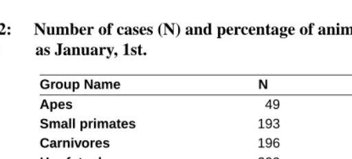
animals based upon age-characteristic behavior and morphology. When an animal with an uncertain birthdate enters a zoo, its birthdate will often be recorded as January 1. Table 2 shows the proportion of animals in each group with a stated birthdate of January 1. Overall, about one in every 24 animals is credited with a January 1 birth date. Clearly, the dating is least precise for crocodilians, where one in five is assigned a January 1 birth date. Apes and small primates have the lowest percentage in this category, suggesting that age assignment is unusually precise for them.
Table 2: Number of cases (N) and percentage of animals with birthdays reported as January, 1st.
Group Name N Percentage
Apes 49 2.37
Small primates 193 1.73
Carnivores 196 2.70
Hoofstock 200 3.26
Kangaroos 114 4.44
Crocodilians 412 18.71
Ratites 208 7.04
Raptors 75 8.68
Total 1,447 4.11
3.
Results
3.1 Life tables for groups of species
To draw a preliminary picture of the characteristic mortality profiles of various large groups of animals, we combine species in the fashion shown in Table 1. The calcula-tion of life tables for these groups is technically straightforward once a decision is made about how to ‘complete’ the life table by adopting an estimate of life expectancy at the oldest ages. A standard procedure is to invoke a relation characteristic of a stationary pop-ulation according to which life expectancy at the beginning of the open-ended age interval is the reciprocal of the death rate above that age (Preston et al., 2001). One problem with this approach in the present circumstance is that relatively few animals contribute obser-vations at very high ages and as result, the estimate of life expectancy at the oldest ages is subject to considerable sampling variability. In addition, the mortality rates at the oldest ages may be biased by measurement problems such as age misreporting or the improper presence in the data set of animals whose death at an earlier age was not registered.
An alternative approach to estimating mortality in the highest age interval is to fit a statistical model to data at younger ages and extrapolate the value of that function into the oldest age interval. The most common statistical function used for this purpose is the Gompertz curve (µ(x) =aebx), which specifies an exponential increase in the mortality hazard with age. In our case the data are too sparse to allow us to distinguish confidently among various competing mortality models. The Gompertz model is chosen because of its simplicity (having only a level and a slope parameter), its familiarity, and the fact that it does a good job of representing adult mortality levels in a wide variety of species (Carnes et al., 1996).
We have applied both approaches to estimate life expectancy at the age that begins the open-ended interval. We select that age to be the lowest integer age above which fewer than 2% of recorded deaths occur. The Gompertz function was fit to the individual-level animal data by using a standard maximum likelihood estimation procedure in STATA. The coefficient of correlation between the two series (N=7) is .89. This value is reassuringly high in view of the fact that the methods of calculation are entirely independent of one another. Except for raptors, for whom the Gompertz model estimates a negative slope of the age-specific death rates, we use the Gompertz values hereafter because the model is parsimonious and provides accurate fit to the data.
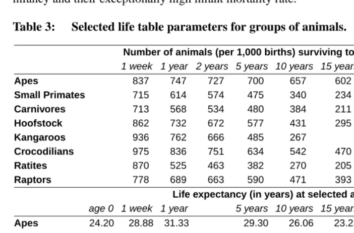
mor-tality among the groups are probably attributable to different ways of recording stillbirths. Nevertheless, the effect of variation in mortality during the first week of life on the rank ordering of life expectancy is small. The ranking of groups from highest to lowest life expectancy at one week of age is nearly the same as the ranking at age zero. By age one, however, ratites have vaulted upwards in the life expectancy rankings as they escape infancy and their exceptionally high infant mortality rate.
Table 3: Selected life table parameters for groups of animals.
Number of animals (per 1,000 births) surviving to different ages
1 week 1 year 2 years 5 years 10 years 15 years 20 years 25 years
Apes 837 747 727 700 657 602 552 473
Small Primates 715 614 574 475 340 234 152
Carnivores 713 568 534 480 384 211 64
Hoofstock 862 732 672 577 431 295 180
Kangaroos 936 762 666 485 267
Crocodilians 975 836 751 634 542 470 399 314
Ratites 870 525 463 382 270 205 144 94
Raptors 778 689 663 590 471 393 353 315
Life expectancy (in years) at selected ages
age 0 1 week 1 year 5 years 10 years 15 years
Apes 24.20 28.88 31.33 29.30 26.06 23.23
Small Primates 8.45 11.80 12.70 11.84 10.58 9.29
Carnivores 7.39 10.34 11.87 9.72 6.50 4.73
Hoofstock 10.05 11.63 12.63 11.59 9.68 7.92
Kangaroos 6.23 6.64 7.06 6.09 4.07 3.08
Crocodilians 19.00 19.47 21.63 24.09 22.77 20.91
Ratites 7.76 8.90 13.45 13.88 12.21 11.59
Raptors 16.57 21.27 22.97 22.77 22.64 21.76
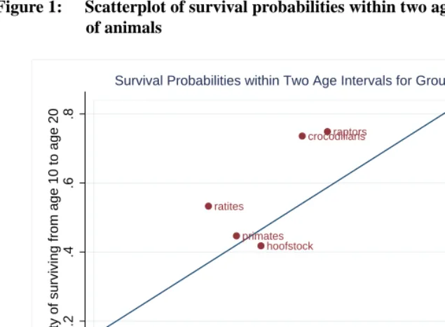
The age-pattern of mortality clearly differs among the groups. Beyond age 5, raptors show little sign of an increase in mortality. Life expectancy at 15 years is nearly the same for them as it is at ages 1, 5, or 10. Crocodilians also show a slow diminution of life expectancy with age. Other groups show a more conventional fall-off in life expectancy as age advances.
Other groups generally fall in an orderly intermediate position with the exception of car-nivores, who have moderate mortality between ages one and ten and quite high mortality between ages 10 and 20.
Figure 1: Scatterplot of survival probabilities within two age intervals for groups of animals
primates
apes
carnivores hoofstock
crocodilians
ratites
raptors
kangaroos
0
.2
.4
.6
.8
Probability of surviving from age 10 to age 20
.4 .6 .8 1
Probability of surviving from age 1 to age 10
Survival Probabilities within Two Age Intervals for Groups of Animals
As theory predicts and as will be demonstrated below, mortality in these heteroge-neous groups rises less rapidly with age than it typically does in the individual species that make up the groups. The most longevous species become relatively more prevalent with age, imparting a downward bias to the age-slope of mortality for the group as a whole (Vaupel and Yashin, 1985).
3.2 Mortality variation by species, sex, and birth type
agexspecified as
µ(x) =h0(x) exp(βzi), (1)
whereh0(x)is the piecewise-constant specification of the baseline hazard with constant mortality risks within one year age intervals, andziare binary variables for sex, birth type or taxonomy of the animal.
The proportional hazard approach enables us to identify how the mortality of each species relates to that of all other species within the group. Other covariates available in the data set that can also be examined are sex and animal’s place of birth (i.e., wild, captivity or unknown place of birth). We estimate the hazard models from age 5 because the proportionality assumption seems less likely to hold across younger ages.
The reference categories that we choose for this analysis (the categories to which all other categories will be compared) are males, animals born in captivity, and the species that contributes the largest number of observations within a group. Animals of unknown sex are excluded from the analysis by sex, but included in other model specifications.
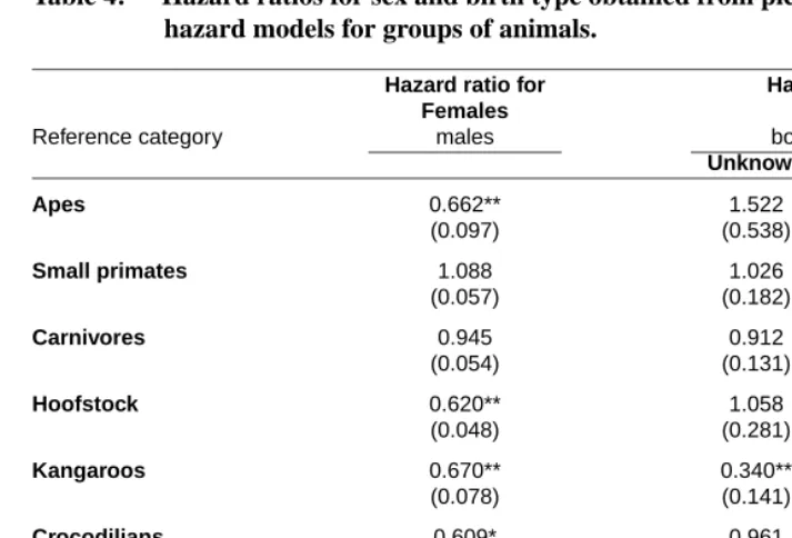
Table 4 shows the coefficients pertaining to sex. Four of the eight groups—apes, hoof-stock, crocodilians, and kangaroos—demonstrate significant sex differences in mortality beyond age five. In each of these cases, females have mortality that is lower than that of males by 33-40%. Sex differences are smaller and insignificant in the remaining groups. Previous studies of sex differences in mortality have typically been based upon fewer ob-servations and indirect indicators, such as the sex ratio of the living population (Taylor and Poole, 1998; Hill et al., 2001; Promislow, 1992). Our results offer partial support to a generalization that has emerged from this literature that males typically have higher mortality among mammals (Promislow, 1992).
There are several reports in the literature of animals who suffer excess mortality when brought into a zoo, relative to animals born and reared in the zoo (Wallace et al., 1987; Tocidlowski et al., 1997; Gozalo and Montoya, 1991). Emotional trauma and exposure to new diets and disease environments are among the causes cited. Table 4 also presents the mortality levels of wild-born animals relative to those of captive-born animals. In none of the groups is the effect of being wild-born statistically significant, and in four of the eight groups the mortality of wild-born animals is lower than that of zoo-born animals. Excess mortality of wild-born animals brought to zoos does not appear to be a general phenomenon. Nevertheless, it should be noted that many of the wild-born animals were brought to a zoo well before the period of observation began. For these animals, any immediate momentary trauma associated with the move would not be reflected in the results.
Table 4: Hazard ratios for sex and birth type obtained from piecewise-constant hazard models for groups of animals.
Hazard ratio for Hazard ratio for
Females Birth Type
Reference category males born in captivity
Unknown Wild born
Apes 0.662** 1.522 1.469
(0.097) (0.538) (0.350)
Small primates 1.088 1.026 1.110
(0.057) (0.182) (0.170)
Carnivores 0.945 0.912 0.887
(0.054) (0.131) (0.096)
Hoofstock 0.620** 1.058 1.294
(0.048) (0.281) (0.418)
Kangaroos 0.670** 0.340** 0.948
(0.078) (0.141) (0.219)
Crocodilians 0.609* 0.961 1.035
(0.142) (0.276) (0.318)
Ratites 1.255+ 1.186 0.811
(0.154) (0.218) (0.328)
Raptors 0.953 0.768 0.638
(0.233) (0.360) (0.222)
Notes: Standard errors in parentheses. p-values:+p <0.05; *p <0.01; **p <0.001.
size of bars corresponding to coefficients larger and smaller than 1. Figure 2 shows that mortality variation is enormous within the group of smaller primates. Mortality rates vary by a factor of nearly eight between brown lemurs at the low extreme and pygmy marmosets at the high. Tamarins are intermediate between the lemurs and the marmosets. In contrast, apes show relatively little differentiation in their post-5 mortality levels, although siamangs have significantly higher mortality than gorillas. Orangutans have mortality that exceeds that of gorillas by 30% but the difference is not statistically sig-nificant. The range of variation is also small among hoofstock. North American bisons, the reference category, have the lowest mortality and gazelles the highest. The group of carnivores shown in Figure 3 also presents a highly varied picture, with bears having very low mortality and cheetahs very high compared to the reference category tigers. Lions and tigers are virtually identical to one another in their post-5 mortality levels.
Differ-Figure 2: Hazard ratios obtained from piecewise-constant model for primates, apes and hoofstock.
hazard ratio 0.52** 0.58** 0.81* 0.85 Ref 1.21+ 1.68** 1.8** 2.31** 2.74** 3.25* 3.97** 4.45** Lion−tailed macaque
Brown lemur Ruffed lemur
Howler monkey
Ring−tailed lemur Colobus monkey
Golden lion tamarin
Sulawesi cr. macaque
G.−headed tamarin
Goeldi’s monkey Dusky titi monkey
Geoffroy’s marmoset Pygmy marmoset 0.5 0.67 1 1.5 2 3 4 5 (a) Primates hazard ratio Ref 1.15 1.3 1.67* Gorilla White−ch. gibbon Orangutan Siamang 1 1.5 (b) Apes hazard ratio Ref 1.25+1.31+ 1.96** 2.81**2.96** 3.48** 6.93**
North Am. bison
Przewalski’s horse
Grevy’s zebra Arabian oryx
Reeves’s muntjac
Eld’s deer
Dorcas gazelle Speke’s gazelle
Figure 3: Hazard ratios obtained from piecewise-constant model for carnivores, crocodilians and ratites.
hazard ratio 0.18** 0.26** 0.34 0.5** 0.62** 0.97 Ref 1.05 1.42+ 1.66* 1.73** 3.1** 3.39** 3.64**
Spectacled bear New Guinea dog
Giant panda Sloth bear
Bobcat
Lion Tiger
Serval
Mexican wolf Leopard cat
Caracal Cheetah
Fishing cat Fennec fox
0.14 0.25 0.5 1 1.5 2 3
4 (d) Carnivores
hazard ratio 0.88 0.89 Ref 1.5 Cuban crocodile Indian gavial American alligator Johnston ’s crocodile 1
1.5 (e) Crocodilians
hazard ratio Ref 1.13 1.9** 4.79** Common emu Cassowary
Greater rhea Darwin
ences in mortality persist also by species among ratites and raptors. Among the non-flying birds (ratites), rheas have the highest mortality levels, and among raptors (not shown here) king vultures have much lower mortality than bald eagles. In summary, significant differ-ences in mortality persist between species within nearly all groups except crocodilians.
3.3 Life table parameters for individual species
In this section we present life table functions for 42 species. This number is lower than the number of species considered in previous sections for the following reasons: a) Crocodil-ians do not show significant inter-species mortality variation, so the four species have been combined into one life table; b), there were too few observations among pandas, New Guinea singing dogs, and dusky titi monkeys (N below 75 in each case) to permit reliable tables to be constructed; c), 98% of the specimens of Darwin’s rhea died before reaching age one, and d), king vultures and howler monkeys had too few observations at older ages to allow life tables to be properly terminated.
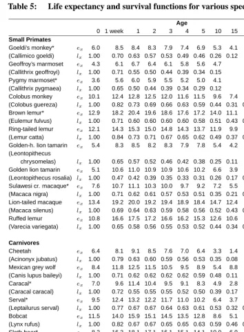
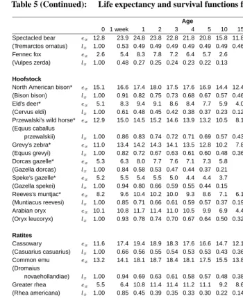
Below age five, the life tables that we construct are based upon directly observed death rates for a species in single years of age (with the first week of life distinguished in infancy). Beyond age five, we used one of two strategies for constructing a life table: con-ventional application of directly observed death rates in single years of age for the species (i.e., the same approach used below age five); or use of the hazard model results for the species. The hazard model approach was employed for the 15 species identified in Table 5 for which the direct use of death rates produced erratic age-patterns of mortality. When di-rect data were used, life tables were terminated in the conventional fashion by estimating life expectancy as the reciprocal of the age-specific death rate in the open-ended interval (Preston et al., 2001). When the hazard model was used, a species’ estimated hazard was assumed to apply in the open-ended interval as well as in all other ages beyond five. In this case, the shape of the hazard was estimated for the group of which the species was a member, and the level of the hazard for the species in question was estimated through the hazard model approach described above. Although results beyond age five are shown in five-year intervals, all calculations are performed in single-year age intervals.
Table 5: Life expectancy and survival functions for various species.
Age
0 1 week 1 2 3 4 5 10 15 20 25 30 35
Small Primates
Goeldi’s monkey* ex 6.0 8.5 8.4 8.3 7.9 7.4 6.9 5.3 4.1 (Callimico goeldi) lx 1.00 0.70 0.63 0.57 0.53 0.49 0.46 0.26 0.12 Geoffroy’s marmoset ex 4.3 6.1 6.7 6.4 6.1 5.8 5.6 4.7 (Callithrix geoffroyi) lx 1.00 0.71 0.55 0.50 0.44 0.39 0.34 0.15 Pygmy marmoset* ex 3.6 5.6 6.0 5.9 5.5 5.2 5.0 4.1 (Callithrix pygmaea) lx 1.00 0.65 0.50 0.44 0.39 0.34 0.29 0.12
Colobus monkey ex 10.1 12.4 12.8 12.5 12.0 11.6 11.5 9.6 7.4 5.0 2.5 (Colobus guereza) lx 1.00 0.82 0.73 0.69 0.66 0.63 0.59 0.44 0.31 0.20 0.09 Brown lemur* ex 12.9 18.2 20.4 19.6 18.6 17.6 17.2 14.0 11.1 8.5 5.9 (Eulemur fulvus) lx 1.00 0.71 0.60 0.60 0.60 0.60 0.58 0.51 0.43 0.34 0.24 Ring-tailed lemur ex 12.1 14.3 15.3 15.0 14.8 14.3 13.7 11.9 9.9 8.6 (Lemur catta) lx 1.00 0.84 0.73 0.71 0.67 0.65 0.62 0.49 0.37 0.25 Golden-h. lion tamarin ex 5.4 8.3 8.5 8.2 8.3 7.9 7.8 5.4 4.2 (Leontopithecus
chrysomelas) lx 1.00 0.65 0.57 0.52 0.46 0.42 0.38 0.25 0.11 Golden lion tamarin ex 5.1 10.6 11.0 10.9 10.9 10.6 10.2 6.6 3.9 2.1 (Leontopithecus rosalia) lx 1.00 0.47 0.42 0.39 0.35 0.33 0.31 0.26 0.17 0.06 Sulawesi cr. macaque* ex 7.6 10.7 11.1 10.3 10.0 9.7 9.2 7.2 5.5 4.0 2.6 (Macaca nigra) lx 1.00 0.71 0.62 0.61 0.57 0.53 0.51 0.35 0.21 0.10 0.03
Lion-tailed macaque ex 13.4 19.2 20.0 19.2 19.4 18.9 18.4 14.7 12.4 9.3 5.1 6.7 4.7 (Macaca silenus) lx 1.00 0.69 0.64 0.63 0.59 0.58 0.56 0.52 0.43 0.36 0.33 0.09 0.04 Ruffed lemur ex 10.8 16.6 17.5 17.2 16.6 16.2 15.3 12.6 10.6 8.8
(Varecia variegata) lx 1.00 0.65 0.58 0.56 0.55 0.53 0.52 0.44 0.34 0.25
Carnivores
Cheetah ex 6.4 8.1 9.1 8.5 7.6 7.0 6.4 3.3 1.4 (Acinonyx jubatus) lx 1.00 0.79 0.63 0.60 0.59 0.56 0.53 0.35 0.08 Mexican grey wolf ex 8.4 11.8 12.5 11.5 10.5 9.5 8.9 5.4 8.8 (Canis lupus baileyi) lx 1.00 0.71 0.62 0.62 0.62 0.62 0.59 0.48 0.11 Caracal* ex 7.0 9.6 11.4 10.4 9.5 9.1 8.3 4.9 2.8 (Caracal caracal) lx 1.00 0.72 0.55 0.55 0.55 0.52 0.50 0.39 0.17 Serval* ex 9.5 12.4 13.2 12.2 11.7 11.0 10.2 6.4 3.7 2.4 (Leptailurus serval) lx 1.00 0.77 0.67 0.67 0.64 0.63 0.61 0.53 0.32 0.09 Bobcat ex 11.5 14.0 15.9 15.1 14.5 13.5 12.8 8.6 5.1 2.9 (Lynx rufus) lx 1.00 0.82 0.67 0.67 0.65 0.65 0.63 0.59 0.46 0.20
Sloth bear* ex 8.2 16.3 18.1 17.1 16.1 15.1 14.1 10.0 6.9 5.6 4.7 3.8 0.8 (Melursus ursinus) lx 1.00 0.50 0.43 0.43 0.43 0.43 0.43 0.40 0.31 0.17 0.08 0.04 0.02 Lion ex 6.4 9.0 11.2 11.9 11.9 11.0 10.5 6.9 3.9 1.7
(Panthera leo) lx 1.00 0.71 0.52 0.45 0.41 0.41 0.39 0.33 0.22 0.07 Tiger ex 9.6 13.3 13.4 12.8 12.0 11.4 10.6 6.5 3.6 2.7 (Panthera tigris) lx 1.00 0.72 0.66 0.64 0.63 0.61 0.60 0.54 0.35 0.08 Leopard cat ex 5.3 7.0 9.4 9.3 8.7 8.7 8.7 5.5 3.5 (Prionailurus
Table 5 (Continued): Life expectancy and survival functions for various species.
Age
0 1 week 1 2 3 4 5 10 15 20 25 30 35
Spectacled bear ex 12.8 23.9 24.8 23.8 22.8 21.8 20.8 15.8 11.8 7.2 3.5 4.1 (Tremarctos ornatus) lx 1.00 0.53 0.49 0.49 0.49 0.49 0.49 0.49 0.46 0.44 0.34 0.06 Fennec fox ex 2.6 5.4 8.3 7.8 7.2 6.4 5.7 2.6
(Vulpes zerda) lx 1.00 0.48 0.27 0.25 0.24 0.23 0.22 0.13
Hoofstock
North American bison* ex 15.1 16.6 17.4 18.0 17.5 17.6 16.9 14.4 12.4 11.7 (Bison bison) lx 1.00 0.91 0.82 0.75 0.73 0.68 0.67 0.57 0.46 0.32 Eld’s deer* ex 5.1 8.3 9.4 9.1 8.6 8.4 7.7 5.9 4.0 (Cervus eldi) lx 1.00 0.61 0.48 0.45 0.42 0.38 0.37 0.23 0.12
Przewalski’s wild horse* ex 12.9 15.0 14.5 15.2 14.6 13.9 13.2 10.5 8.1 6.3 4.3 3.2 (Equus caballus
przewalskii) lx 1.00 0.86 0.83 0.74 0.72 0.71 0.69 0.57 0.43 0.27 0.16 0.05 Grevy’s zebra* ex 11.0 13.4 14.2 14.3 14.1 13.5 12.8 10.2 7.8 6.1 4.2 3.1 (Equus grevyi) lx 1.00 0.82 0.72 0.67 0.63 0.61 0.60 0.48 0.36 0.22 0.13 0.04 Dorcas gazelle* ex 5.3 6.3 8.0 7.7 7.6 7.1 7.3 5.8
(Gazella dorcas) lx 1.00 0.84 0.58 0.53 0.47 0.44 0.37 0.21 Speke’s gazelle* ex 5.2 5.5 5.4 5.5 5.0 4.4 4.4 3.7 (Gazella spekei) lx 1.00 0.94 0.80 0.66 0.59 0.55 0.44 0.15 Reeves’s muntjac* ex 8.2 9.6 10.4 10.2 10.0 9.3 8.6 7.1 6.1 (Muntiacus reevesi) lx 1.00 0.85 0.71 0.66 0.61 0.59 0.57 0.37 0.19 Arabian oryx ex 10.1 10.8 11.7 11.4 11.0 10.5 9.9 6.9 4.4 (Oryx leucoryx) lx 1.00 0.93 0.78 0.74 0.70 0.67 0.64 0.50 0.32
Ratites
Cassowary ex 11.6 17.4 19.4 18.9 18.3 17.6 16.6 14.7 12.1 10.1 6.8 3.5 (Casuarius casuarius) lx 1.00 0.66 0.56 0.55 0.54 0.53 0.53 0.43 0.36 0.28 0.23 0.16 Common emu ex 13.2 14.1 18.1 18.7 18.4 18.1 17.5 15.5 13.8 11.3 11.0 9.1 (Dromaius
novaehollandiae) lx 1.00 0.94 0.69 0.63 0.61 0.58 0.57 0.48 0.38 0.31 0.21 0.15 Greater rhea ex 5.5 6.4 10.8 11.4 11.4 11.2 11.1 9.2 8.6
(Rhea americana) lx 1.00 0.85 0.45 0.39 0.35 0.33 0.30 0.22 0.14
Raptors
Bald eagle ex 13.2 17.3 19.0 18.9 19.0 19.0 18.8 18.8 17.3 14.2 10.8 8.7 7.6 (Haliaeetus
leucocephalus) lx 1.00 0.76 0.66 0.63 0.59 0.56 0.54 0.41 0.34 0.31 0.27 0.20 0.12
Kangaroos
Western grey kangaroo* ex 7.3 7.8 8.5 8.7 8.2 7.9 7.7 5.5 4.8 (Macropus fuliginosus) lx 1.00 0.93 0.76 0.66 0.62 0.57 0.52 0.33 0.15 Red kangaroo ex 6.0 6.4 6.8 6.7 6.5 6.2 5.9 4.0 (Macropus rufus) lx 1.00 0.94 0.76 0.67 0.59 0.53 0.47 0.25
high mortality at or shortly after birth and only 53% of the animals survive to one week of age. A similar pattern is observed for the sloth bear and the fennec fox among whom only half of the born cubs survive the first week of their life. Among small primates, the golden-lion tamarin is characterized by the highest mortality between birth and one week of age. Lions and tigers have very similar mortality beyond age three although lions have higher death rates below that age.
Not all remaining species are shown in Table 5 because several important species do not exhibit enough deaths at older ages during the period under study to enable the life table to be properly completed. This pattern is observed among crocodilians and apes. In these species, the recorded death rates during the 1998-2003 period imply that large numbers would survive to older ages. However, in the zoo collections during the period under investigation, there are too few deaths at those older ages to allow the life table to be confidently closed out. For example, the life table for gorillas indicates that 31% will survive to age 40, but in the populations and period under study there were only 146 years of exposure and 9 deaths recorded above age 40.
There are several possible explanations of this anomaly: a) Death rates for a species were unusually low during the period 1998-2003; the shortage of very old specimens during this period is a result of higher death rates during earlier periods. b) Deaths are underrecorded; c) The number of specimens is overestimated. This latter problem would be particularly serious if specimens who had died or out-migrated were erroneously main-tained on a zoo’s books. In this case, the fraction of estimated years at risk that consisted of absent animals would grow as age advances, and death rates at older ages would be progressively biased downwards.
We consider it unlikely that deaths in these species were underrecorded because four of the five species affected by the problem are apes who are often among the most visible and important species in a collection. In the case of gorillas, it seems more likely that the ISIS data base includes inaccurate records of survivors. Gorillas are assigned multiple studbook numbers in various regions around the world, which is a source of confusion in the record system (Flesness et al., 1995). One analysis argues that "...the mish mosh of studbook IDs that presently permeates the ISIS database for gorillas does not permit either genetic or demographic analyses for one of the highest profile and most charismatic megavertabrates in captivity." (Earnhardt et al., 1995).
the recorded survival for these species and the number of older specimens in collections means that the results, shown in Table 6, are less reliable than for other species presented.
Table 6: Partial life expectancy and survival functions for Apes and Crocodilians.
Age
0 1 week 1 2 3 4 5 10 15 20 25 30 35 40
Apes
Gorilla ex23.3 27.2 29.1 28.7 28.1 27.1 26.4 22.7 19.1 15.3 12.1 8.3 4.4 0* (Gorilla gorilla) lx 1.00 0.86 0.77 0.76 0.75 0.75 0.74 0.70 0.65 0.61 0.54 0.48 0.40 0.31* White-ch. gibbon ex15.3 20.4 21.9 22.8 21.8 20.8 20.5 16.6 12.8 8.7 4.7 0*
(Hylobates
leucogenys) lx 1.00 0.75 0.67 0.61 0.61 0.61 0.59 0.56 0.51 0.47 0.41 0.36 Siamang ex19.5 22.2 23.7 23.0 22.3 21.3 21.0 17.7 14.6 11.1 8.2 4.4 0* (Hylobates
syndactylus) lx 1.00 0.88 0.79 0.78 0.77 0.77 0.74 0.68 0.60 0.54 0.43 0.36 0.26* Orangutan ex19.0 23.6 26.3 26.0 25.3 25.5 24.5 21.0 17.8 14.3 11.4 7.9 4.3 0* (Pongo pygmaeus)lx 1.00 0.80 0.69 0.67 0.67 0.64 0.64 0.59 0.54 0.50 0.42 0.36 0.28 0.20*
Crocodilians ex14.6 14.9 16.4 17.2 17.9 17.7 17.1 14.6 11.5 8.1 4.5 0*
lx 1.00 0.97 0.84 0.75 0.68 0.65 0.63 0.54 0.47 0.40 0.31 0.25*
Notes: * By assumption; The group of crocodilians includes American alligator, Johnston’s crocodile, Cuban crocodile and Indian gavial.
Despite the assumption that no years would be lived beyond age 40 by a cohort of newborn gorillas, the gorilla life expectancy at birth, 23.3 years, is the highest of any species considered. Likewise, orangutans, gibbons, and siamangs achieve a higher life expectancy at birth than any other species under review despite having their survivorship artificially truncated. These species of apes also provide four out of the five highest life expectancies at one week of age (with spectacled bears). Clearly, apes appear to live longer in captivity than the other species that we have reviewed, but data inconsistencies add uncertainty to this conclusion.
4.
Discussion
Figure 4 compares our estimates of life expectancy at age one week for mammalian species to estimates of the highest age attained by that species (N=37). Life expectancy at age one week is used rather than at age zero in order to minimize the influence of fetal mortality. The relationship is tight, with a coefficient of correlation between the two series of .87. The line fitted on the graph indicates that the average length of life of a species is approximately equal to half of the highest age attained by that species. For the many mammalian species not included in this analysis and for whom no reliable life table has been constructed but for whom a maximum attained age has been estimated, this rule of thumb may prove useful.
Figure 4: Relationship between life expectancy and highest age ever attained by mammalian species.
However, non-mammalian species show a much poorer fit between these two vari-ables, with a correlation of only .55 (N=5). It is possible that the fit is poorer because Carey and Judge were unable to observe as many members of these species as of mam-mals, adding greater variability to their estimates. For mammals and non-mammals com-bined, the correlation coefficient is .77.
References
Carey J R, Judge D S. 2000. Longevity Records: Life Spans of Mammals, Birds, Am-phibians, Reptiles, and Fish. Odense: Monographs on Population Aging 8, Odense University Press.
Carnes B A, Olshansky S J, Grahn D. 1996. Continuing the search for a law of mortality. Population and Development Review 22:231–264.
Courteney J, Santow G. 1989. Mortality of wild and captive chimpanzees. Folia Prima-tologica 52:167–177.
de Wit J J. 1995. Mortality of rheas caused by a synchamus trachea infection. Veterinary Quarterly 17:39–40.
Earnhardt J M, Thompson S D, Willis K. 1995. Reply to Flessness et al. Zoo Biology 14:519–522.
Ernest, S K. Morgan 2003. Life History Characteristics of Placental Nonvolant Mammals. Ecology 84:3402.
Flesness N R, Lukens D R, Porter S B, Wilson C R, Grahn L V. 1995. ISIS and stud-books, very high census correlation for the north american zoo population: a reply to Earnhardt, Thompson, and Willis. Zoo Biology 14:509–517.
Felsenstein, J. 1985. Phylogenies and the Comparative Method. The American Naturalist 125:1-15.
Gozalo A, Montoya E. 1991. Mortality causes of the moustached tamarin (Saguinus mystax) in captivity. Journal of Medical Primatology 21:35–38.
Hill K, Boesch C, Goodall J A, Pusey A, Williams J, Wrangham R. 2001. Mortality rates among wild chimpanzees. Journal of Human Evolution 40(5): 437–450.
Karstad L, Sileo L. 1971. Causes of death in captive wild waterfowl in the Kortright Waterfowl Park, 1967-1970. Journal of Wildlife Diseases 7:236–241.
Leong K M, Terrell S P, Savage A. 2004. Causes of mortality in captive cotton-top tamarins (Saguinus oedipus). Zoo Biology 23:127–137.
Preston S H, Heuveline P., Guillot M. 2001. Demography: Measuring and Modeling Population Processes. Oxford: Blackwell Publishers.
Taylor V J, Poole T B. 1998. Captive breeding and infant mortality in Asian elephants; A comparison between twenty Western zoos and three Eastern elephant centers. Zoo Biology 17:311–332.
Tocidlowski M E, Cornish T E, Loomis M R, Stoskopf M K. 1997. Mortality in cap-tive wild-caught horned puffin chicks (Fratercula Corniculata). Journal of Zoo and Wildlife Medicine 28:298–306.
Vaupel J W, Yashin A I. 1985. Heterogeneity’s ruses: Some surprising effects of selection on population dynamics. American Statistician 39:176–185.
Wallace R S, Bush M, Montali R J. 1987. Deaths from exertional myopathy at the National Zoological Park from 1975 to 1985. Journal of Wildlife Diseases 23:454–462.
Ward M P, Ramer J C, Proudfoot J, Garner M M, Juan-Sallès C, Wu C C. 2003. Outbreak of salmonellosis in a zoologic collection of Lorikeets and Lories (Trichoglossus, Lorius, and Eos spp.). Avian Diseases 47:493–498.
[WHO] World Health Organization. 1977. Manual of Mortality Analysis. Geneva: Divi-sion of Health Statistics, World Health Organization.