Volume 29 - Article 30 | Pages 817–836

(1)

DEMOGRAPHIC RESEARCH

VOLUME 29, ARTICLE 30, PAGES 817-836

PUBLISHED 15 OCTOBER 2013

http://www.demographic-research.org/Volumes/Vol29/30/ DOI: 10.4054/DemRes.2013.29.30

Research Article

All tied up: Tied staying and tied migration

within the United States, 1997 to 2007

Thomas J. Cooke

This open-access work is published under the terms of the Creative Commons Attribution NonCommercial License 2.0 Germany, which permits use, reproduction & distribution in any medium for non-commercial purposes, provided the original author(s) and source are given credit.

(2)

1 Introduction 818

2 Background 819

3 Research strategy 821

4 Data and methods 823

5 Results 826

6 Conclusion 831

(3)

All tied up:

Tied staying and tied migration within the United States,

1997 to 2007

Thomas J. Cooke1

Abstract

BACKGROUND

The family migration literature presumes that women are cast into the role of the tied migrant. However, clearly identifying tied migrants is a difficult empirical task, since it requires the identification of a counterfactual: who moved but did not want to?

OBJECTIVES

This research develops a unique methodology to directly identify both tied migrants and tied stayers in order to investigate their frequency and determinants.

METHODS

Using data from the 1997 through 2009 U.S. Panel Study of Income Dynamics (PSID), propensity score matching is used to match married individuals with comparable single individuals to create counterfactual migration behaviors: who moved but would not have moved had they been single (tied migrants) and who did not move but would have moved had they been single (tied stayers).

RESULTS

Tied migration is relatively rare and not limited just to women: rates of tied migration are similar for men and women. However, tied staying is both more common than tied migration and equally experienced by men and women. Consistent with the body of empirical evidence, an analysis of the determinants of tied migration and tied staying demonstrates that family migration decisions are imbued with gender.

CONCLUSIONS

Additional research is warranted to validate the unique methodology developed in this paper and to confirm its results. One line of future research should be to examine the effects of tied staying, along with tied migration, on well-being, union stability, employment, and earnings.

(4)

1. Introduction

Migration is rarely an individual event. Decisions to move, and their consequences, are usually embedded within the context of the family. According to the 2012 U.S. Current Population Survey at least 94% of all inter-county migration events in the United States occur among individuals who are either members of a family or non-family members who moved for ―family reasons‖2. The family dimension of migration is important to recognize as it contains both social and economic dimensions that are frequently ignored in internal migration research. One important aspect of family migration decisions and their consequences is that they are conditioned on the employment and earnings capacity of spouses relative to their gender ideologies (Bielby and Bielby 1992; Bird and Bird 1985; Bonney and Love 1991; Cooke 2008a; Jurges 2006; Wallston, Foster, and Berger 1978). Thus, the family migration literature has traditionally presumed that migrant wives are disproportionately cast into the role of the tied migrant (Cooke 2008b), which in turn contributes to the gender gap in earnings (Cooke et al. 2009).

However, gender role attitudes are slowly becoming more egalitarian (Cotter, Hermsen, and Vanneman 2011), dual-earner families are becoming the norm (U.S. Bureau of Labor Statistics 2011), and the number of families in which the wife is the primary earner is increasing (U.S. Bureau of Labor Statistics 2011). These trends have several consequences. They imply that married women should be less often cast into the role of the trailing wife and this might have a positive impact on the gender gap in earnings. As well, they suggest an increase in the number of tied stayers (spouses who desire to move but cannot because other family members do not want to move), which may be a contributing factor in the long-term decline in U.S. internal migration rates (Cooke forthcoming-a). In turn, the decline in internal migration rates due to the growing immobility of dual-earner couples may result in the inefficient allocation of labor across regional labor markets, which may then contribute to an increase in regional labor market inequality (Cherry and Tsournos 2001; Cooke forthcoming-b). Thus, far from being an esoteric subfield of migration studies, the changing social and economic context within which family migration decisions are made has wide-ranging impacts.

This research focuses on an important and vexing problem within the family migration literature: identifying tied migrants and tied stayers. A tied migrant is usually defined as an individual whose family migrated but who would not have chosen to move if single, and a tied stayer is an individual whose family did not migrate but who

(5)

would have migrated if single. Identifying either is a daunting empirical task because this requires the identification of a difficult to observe counterfactual: what would be the migration behavior of a married person had they not been married? This research uses methods from the propensity score matching literature to match married individuals with comparable single individuals to create those counterfactuals. These counterfactual data are then used to examine the frequency of tied migration and tied staying and to examine their causes.

This research makes four important contributions to both the family migration literature and migration research in general. First, despite the family migration literature’s focus on the trailing wife, this is the first study to provide a method for identifying tied migrants and for directly measuring the causes of tied migration. Second, the family migration literature has tended to focus on women as tied migrants. This empirical analysis allows for the increasing likelihood that men are tied migrants. As such, it brings men more clearly into discussions of the causes of tied migration, allowing for a more nuanced consideration of the role of gender in shaping family migration behavior. Third, the family migration literature focuses exclusively on tied migration at the expense of tied staying, perhaps because tied staying is so much more difficult to conceptualize than tied moving. However, theoretically the effects of tied staying are no less significant than the effects of tied staying. This analysis provides a clear method to identify tied staying and to assess its frequency. Finally, migration research in general treats migration as having binary properties. Migration and migrants are treated as having qualities that are absent from staying and stayers. By identifying tied stayers this research points toward an expanded discussion away from the effects of moving and toward the effects of staying.

2. Background

(6)

effect of the husband’s and wife’s characteristics on the decision to move should be symmetrical. That is, for example, the effect of the wife’s education on migration should be the same as the husband’s.

However, the earliest empirical research found that families were largely unresponsive to measures of the wife’s human capital when making migration decisions and that migration decisions were largely a function of the husband’s human capital (Duncan and Perrucci 1976; Lichter 1980; Lichter 1982; Long 1974; Spitze 1984). This implied that family migration was tilted in favor of the husband’s employment and earnings, a hypothesis that has been supported by a large body of research on the effects of family migration on the wife’s earnings and employment (see Cooke (2008b) for a review of the literature and Taylor (2007), McKinnish (2008), Blackburn (2009), Blackburn (2010), Boyle, Feng, and Gayle (2009), Cooke et al. (2009), Rabe (2011), and Eliasson et al. (forthcoming) for more recent studies). These findings have led to the development of a gendered model of family migration, which is supported by several studies that find a strong effect of gender role beliefs in mediating the effects of the husband’s and wife’s human capital in shaping the migration decision (Bielby and Bielby 1992; Bird and Bird 1985; Bonney and Love 1991; Cooke 2008a; Jurges 2006; Wallston, Foster, and Berger 1978). However, gender role attitudes have slowly become more egalitarian (Cotter, Hermsen, and Vanneman 2011). The implication is that family migration decisions should have become more consistent with the human capital model over time. And, indeed, more recent studies, with a few important exceptions (Compton and Pollak 2007; Nivalainen 2004; Shauman 2010), have found that the relative effect of the husband’s and wife’s human capital characteristics in shaping the migration decision has become more symmetrical (Brandén 2013; Eliasson et al. forthcoming; Rabe 2011; Smits, Mulder, and Hooimeijer 2003; Smits, Mulder, and Hooimeijer 2004; Swain and Garasky 2007).

(7)

through the application of propensity score matching to provide the counterfactual migration behavior for married men and women. This approach is used to examine the frequency of tied migration and tied staying by gender and to explore the causes of tied migration and tied staying. Of particular interest is to evaluate the gender distribution in rates of tied migration and tied staying and to examine how status as a tied migrant or as a tied stayer is linked to human capital characteristics apart, or together, with gender.

3. Research strategy

Propensity score matching attempts to create matched control-treatment pairs from secondary data sources, and then to treat them statistically as if they were produced from a controlled experimental study in order to observe the effect of receiving the treatment relative to not receiving the treatment (Rosenbaum and Rubin 1983; Rosenbaum and Rubin 1985). Propensity score matching starts by estimating a model of being in a treatment group relative to being in a control group as a function of observed variables that affect both the probability of being in the treatment group and the outcome (Heinrich, Maffioli, and Vazquez 2010). The resulting predicted probability of inclusion in the treatment group (the propensity score) is then used to match individuals in the treatment group to individuals in the control group. Using the example at hand, the idea is that if a person who is actually married has a predicted probability of being married of only 30% and is matched to a single individual who also has a predicted probability of being married of only 30%, then differences in the outcome (migration) are not due to observable differences between the unmarried and married individuals but only due to whether the individual is actually married or not. Statistically, the veracity of this argument hinges on the degree to which the model of being in the treatment group includes the appropriate set of observable variables (Morgan and Winship 2007).

However, this research is not as interested in the differences in the outcomes between the treatment and control groups but in using the matched treatment-control data to identify tied migrants and tied stayers. In this context:

 Tied Stayers are married individuals who did not migrate but whose single match did migrate;

 Tied Migrants are married individuals who migrated but whose single match did not migrate;

(8)

 Migrants are married individuals who migrated and whose single match also migrated.

Thus, this procedure allows for the identification of the counterfactual that has to date eluded family migration research: who moved but would not have moved had they been single (tied movers) and who stayed but would have moved had they been single (tied stayers)?

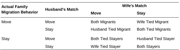
However, status across these four categories varies within each couple. Following Table 1, families are further classified as:

 Both Stayers: The family did not migrate and both the husband and wife are matched to non-migrants;

 Both Migrants: The family migrated and both the husband and wife are matched to migrants;

 Wife Tied Stayer: The family did not migrate, the husband is matched to a non-migrant, and the wife is matched to a migrant;

 Husband Tied Stayer: The family did not migrate, the husband is matched to a migrant, and the wife is matched to a non-migrant;

 Both Tied Stayers: The family did not migrate and both the husband and the wife are matched to migrants;

 Wife Tied Migrant: The family migrated, the husband is matched to a migrant, and the wife is matched to a non-migrant;

 Husband Tied Migrant: The family migrated, the husband is matched to a non-migrant, and the wife is matched to a migrant; and

 Both Tied Migrants: The family migrated and both the husband and wife are matched to migrants.

Table 1: Classification of family migration behavior

Actual Family

Migration Behavior Husband's Match

Wife's Match

Move Stay

Move Move Both Migrants Wife Tied Migrant

Stay Husband Tied Migrant Both Tied Migrants

Stay Move Both Tied Stayers Husband Tied Stayer

Stay Wife Tied Stayer Both Stayers

(9)

4. Data and methods

Data for the analysis are drawn from the U.S. Panel Study of Income Dynamics (PSID). The PSID is a national study of U.S. households. Beginning in 1968, around 18,000 individuals living in 5,000 households were sampled annually through 1997 and biannually since then. The sample includes the descendants of original sample members, and so the 2009 sample has grown to include more than 9,000 households and 24,000 individuals. With the addition of descendants of original sample members the sample is not representative of the U.S. population, requiring the use of either individual or family weights, when appropriate, to approximate the characteristics of the U.S. population. In order to define migration at a fine geographic scale – the county level in this case – the analysis relies upon a restricted use geocoded version of the PSID.3 Specifically, this analysis conducts the matching procedure on a pooled sample of the 1997 through 2009 PSID, defining migration as a prospective change in county of residence from one panel to the next. All variables are based upon the county of residence prior to observing any migration behavior. The sample is restricted to married and single individuals between 25 and 64, inclusive, whose marital status did not change from one panel to the next. Cohabiting couples are excluded. The sample is further limited to whites because the PSID inconsistently samples and identifies non-whites between 1997 and 2009.

Propensity score matching takes place in four iterative steps (Heinrich, Maffioli, and Vazquez 2010): 1) estimating a model of the probability of receiving the treatment versus not receiving the treatment, 2) using these probabilities to match individuals receiving the treatment to those not receiving the treatment, 3) evaluating the quality of these matches, and 4) if the quality of the matches is not adequate, identifying different model and matching specifications until the matches meet appropriate statistical criteria. Of central importance is the specification of the model of the probability of receiving the treatment (Morgan and Winship 2007). Strictly speaking, the model should include variables that 1) determine the outcome, 2) are either fixed or measured prior to the treatment, and 3) are not affected by either the treatment or the outcome (Brookhart et al. 2006). In the context of this analysis these are strict and would severely limit the ability to conduct the analysis (e.g., they would preclude the inclusion of parental status in the analysis). However, these restrictions are in place to ensure that the comparisons of the outcomes between the treated and control groups are unbiased. In this case, however, the focus is on identifying appropriate counterfactual matches

(10)

and these restrictions are relaxed to include variables that are not directly determined by the treatment or outcome in any particular year. For example, the model of the probability of receiving the treatment versus not receiving the treatment includes the ages of children – which can predate marriage and which are not solely determined by marital status – but excludes employment status, which is directly affected by marital status, especially for women.

Within this framework the independent variables determining the probability of migration are as follows: age (categorized into five-year increments), housing tenure (=1 if owner occupied), education (=1 if college graduate), gender (=1 if female), presence of a young child in the household (=1 if youngest child in the household is aged 1 through 5), presence of an older child in the household (=1 if youngest child in the household is aged 6 through 17), and a measure of previous migration history. Specifically, previous residential history is defined as whether the individual is living in the same state in which either parent grew up (=1 if yes). This is both a reflection of previous migration history and potential personal and family ties to the state.

This said, there are actually two ways to conduct the matching. One way is to include all relevant variables in the model of the probability of receiving the treatment and to match on that probability. However, in many cases it is necessary to stratify the matching by selected independent variables to prevent irrelevant matches or to improve matching outcomes. In the first case the analysis is stratified by year and gender to make sure that married individuals are matched to single individuals who share a common year and gender. In the second case the analysis is further stratified by age and educational status to improve the matching outcomes. Thus, within each of the strata defined by age, gender, year, and education, a logit model of the probability of receiving the treatment as a function of housing tenure and age of youngest child is estimated.4 Finally, using the PSMATCH2 Stata module (Leuven and Sianesi 2003; StataCorp 2011) a nearest neighbor algorithm matches single individuals to married individuals within each strata based upon the predicted odds of being married. In cases where there is more than one potential single match to a married individual, one of these single matches is randomly selected to serve as the match.

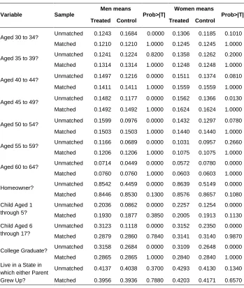
Table 2 reports on the quality of the matching procedure by comparing the means of the explanatory variables between the treated and control groups by gender. The logic behind propensity score matching is clearly demonstrated at this point. The unmatched samples show large differences in the characteristics of the married and unmarried samples, many of which are statistically significant. Comparing any outcome across these two groups would be statistically unwise. However, after matching these two samples are nearly identical in every observable way, except for the fact that one

(11)

group is married and the other is not. Indeed, none of these differences are statistically significant.

Table 2: Evaluation of matching criteria

Variable Sample

Men means

Prob>|T|

Women means

Prob>|T|

Treated Control Treated Control

Aged 30 to 34? Unmatched 0.1243 0.1684 0.0000 0.1306 0.1185 0.1010

Matched 0.1210 0.1210 1.0000 0.1245 0.1245 1.0000

Matched 0.1314 0.1314 1.0000 0.1248 0.1248 1.0000

Matched 0.1411 0.1411 1.0000 0.1559 0.1559 1.0000

Matched 0.1492 0.1492 1.0000 0.1624 0.1624 1.0000

Matched 0.1503 0.1503 1.0000 0.1440 0.1440 1.0000

Matched 0.1206 0.1206 1.0000 0.1075 0.1075 1.0000

Matched 0.0760 0.0760 1.0000 0.0603 0.0603 1.0000

Homeowner? Unmatched 0.8542 0.4459 0.0000 0.8639 0.5149 0.0000

Matched 0.8446 0.8530 0.1300 0.8576 0.8657 0.1080

Child Aged 1 through 5?

Unmatched 0.2036 0.0862 0.0000 0.2257 0.1254 0.0000

Matched 0.1930 0.1877 0.3850 0.2005 0.1913 0.1130

Unmatched 0.3123 0.1118 0.0000 0.3152 0.2350 0.0000

Matched 0.2879 0.2860 0.7840 0.3141 0.3140 0.9870

College Graduate? Unmatched 0.3158 0.2684 0.0000 0.3109 0.2648 0.0000

Matched 0.2865 0.2865 1.0000 0.2840 0.2840 1.0000

Live in a State in which either Parent Grew Up?

Unmatched 0.4137 0.4038 0.3700 0.4293 0.4130 0.1340

(12)

5. Results

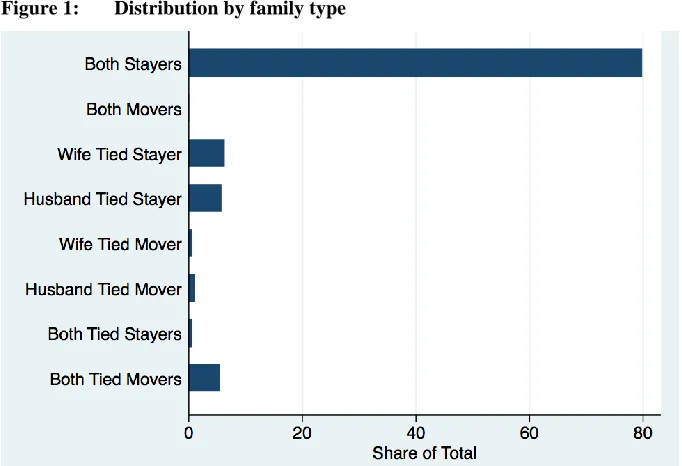
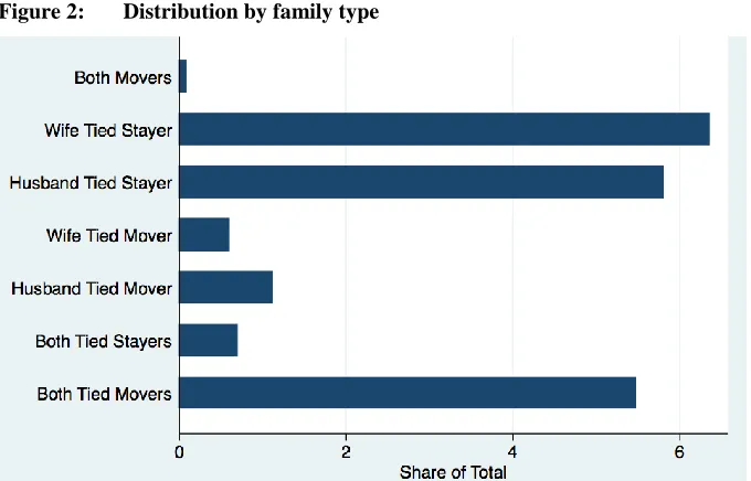
Figure 1 shows the distribution of married couples across the eight classifications presented in Table 1. Both Stayers dominate the distribution, as most married couples consist of individuals who did not move and who were matched to single individuals who also did not move. Figure 2 highlights the balance of family types by excluding the category of Both Stayers. Several important trends are displayed in the results. Despite the family migration literature’s focus on female tied migrants, this is a relatively rare event. Rather, most women are tied movers in combination with their husbands also being tied movers (i.e., they are Both Tied Migrants). Indeed, men are just as likely to be tied movers as are women. Furthermore, rates of tied staying are much higher than rates of tied moving – for both men and women.

(13)

Figure 2: Distribution by family type

(14)

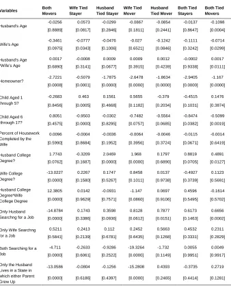
Table 3: Multinomial logit models of family type

Parameter Estimates - Relative to Both Stayers [p-value*]

Variables Both Movers Wife Tied Stayer Husband Tied Stayer Wife Tied Mover Husband Tied Mover Both Tied Stayers Both Tied Movers Husband's Age

-0.0256 0.0573 -0.0299 -0.0867 -0.0854 -0.0137 -0.1098 [0.8889] [0.0817] [0.2846] [0.1811] [0.2441] [0.8647] [0.0004]

Wife's Age -0.3461 -0.0777 -0.0476 -0.027 -0.1242 -0.1111 -0.0714 [0.0975] [0.0343] [0.1006] [0.6521] [0.0846] [0.3242] [0.0299] Husband's Age

*Wife's Age

0.0017 -0.0008 0.0009 0.0009 0.0012 -0.0002 0.0017 [0.6890] [0.3141] [0.0677] [0.3915] [0.4239] [0.9338] [0.0111]

Homeowner?

-2.7221 -0.5079 -1.7875 -2.6478 -1.8634 -2.9405 -1.167 [0.0008] [0.0001] [0.0000] [0.0000] [0.0000] [0.0000] [0.0000]

-0.2683 0.463 0.1561 0.5655 -0.379 -0.4515 0.1476 [0.8456] [0.0005] [0.4668] [0.1182] [0.2034] [0.1031] [0.3874] Child Aged 6

through 17?

0.8051 -0.9503 -0.0302 -0.7482 -0.5564 -0.8474 -0.5099 [0.4575] [0.0000] [0.8295] [0.0757] [0.0685] [0.0382] [0.0019] Percent of Housework

Completed by the Wife

0.0096 -0.0004 -0.0036 -0.0064 -0.0046 -0.0115 -0.0014 [0.5990] [0.8684] [0.1952] [0.3956] [0.3724] [0.0671] [0.6419] Husband College

Degree?

1.7743 -0.3209 2.0469 1.968 0.1797 0.8819 0.4891 [0.0762] [0.1687] [0.0000] [0.0000] [0.6890] [0.0705] [0.0127] Wife College

Degree?

-13.0227 0.2267 0.1747 0.8458 0.0137 -0.4927 0.1123 [0.0000] [0.1580] [0.5267] [0.1011] [0.9738] [0.3739] [0.5691] Husband College

Degree*Wife College Degree

12.3805 0.0142 -0.0931 -1.147 0.0697 0.4596 -0.1614 [0.0000] [0.9629] [0.7571] [0.0860] [0.9106] [0.5495] [0.5702] Only Husband

Searchng for a Job

-14.8784 0.1743 0.3598 0.8128 0.7877 0.6173 0.6656 [0.0000] [0.3386] [0.0936] [0.0612] [0.0151] [0.1463] [0.0002] Only Wife Searchng

for a Job

0.5211 0.2413 0.112 0.2452 0.5663 0.4532 0.2311 [0.5841] [0.2139] [0.6781] [0.6435] [0.1268] [0.3331] [0.2829] Both Searching for a

Job

-4.711 -0.2633 -0.9286 -19.3264 -1.732 0.0055 0.0049 [0.0000] [0.6061] [0.2522] [0.0000] [0.1149] [0.9951] [0.9917] Only the Husband

Lives in a State in which either Parent Grew Up

(15)

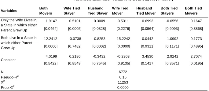
Table 3: Continued

Parameter Estimates - Relative to Both Stayers [p-value*]

Variables Both Movers Wife Tied Stayer Husband Tied Stayer Wife Tied Mover Husband Tied Mover Both Tied Stayers Both Tied Movers

Only the Wife Lives in a State in which either Parent Grew Up

1.9147 0.5101 0.3009 0.5311 0.6993 -0.0556 0.1647 [0.0464] [0.0005] [0.0328] [0.2276] [0.0564] [0.9093] [0.3868] Both Live in a State in

which either Parent Grew Up

12.2412 -0.0738 -0.8253 15.2242 0.0442 1.0992 0.1773 [0.0000] [0.7482] [0.0002] [0.0000] [0.9311] [0.1171] [0.4895]

Constant

4.0199 0.2180 -0.3432 -0.2303 3.4530 2.9242 2.7074 [0.5422] [0.8549] [0.7545] [0.9135] [0.1417] [0.3571] [0.0195]

N 6772

Pseudo-R2 0.15 X2 11253 Prob>X2 0.0000

Notes: * Standard errors are adjusted for the clustering of observations across panels by household.

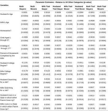
Interpreting multinomial logit models is complex because the results are presented either in log-odds or odds ratios and the parameters are relative to the base category (i.e., Both Stayers). Therefore, the results are recalculated as average marginal effects in Table 4. Average marginal effects are calculated for each focal variable by estimating the probability of being in a particular family type under two scenarios: holding the focal variable at a value of zero and then again at a value of one while allowing all other values to remain as observed. For each observation the difference in the predicted probability of being in a particular family type under each scenario is calculated. These differences are then averaged across the sample using PSID household weights. The advantage of using average marginal effects in this case is that they incorporate the interaction variables, they are in terms of probabilities, and are relative to all other family types rather than the base category.

(16)

This suggests that families are ignoring this characteristic of the wife when making the decision to stay.

Table 4: Marginal effects of logit models of family type

Variables

Parameter Estimates - Relative to All Other Categories [p-value]

Both Stayers Both Movers Wife Tied Stayer Husband Tied Stayer Wife Tied Mover Husband Tied Mover Both Tied Stayers Both Tied Movers Husband's Age

0.0001 0.0000 0.0018 0.0009 -0.0003 -0.0004 -0.0001 -0.0020 [0.9394] [0.6825] [0.0090] [0.2530] [0.2519] [0.3404] [0.7248] [0.0085]

Wife's Age 0.0057 -0.0002 -0.0057 0.0004 0.0002 -0.0006 -0.0006 0.0009 [0.0000] [0.0994] [0.0000] [0.6356] [0.4109] [0.1696] [0.0456] [0.2655]

Homeowner? 0.2432 -0.0022 -0.0045 -0.1199 -0.0246 -0.0202 -0.0210 -0.0508 [0.0000] [0.1020] [0.5476] [0.0000] [0.0000] [0.0000] [0.0000] [0.0000] Child Aged 1

through 5?

-0.0389 -0.0002 0.0329 0.0057 0.0042 -0.0052 -0.0039 0.0053 [0.0284] [0.7961] [0.0009] [0.6128] [0.2136] [0.0876] [0.0472] [0.5800] ChildAge 6

through 17?

0.0633 0.0015 -0.0385 0.0037 -0.0029 -0.0041 -0.0042 -0.0188 [0.0000] [0.3478] [0.0000] [0.6083] [0.1103] [0.2246] [0.1091] [0.0078] Percent of Housework

Completed by the Wife

0.0003 0.0000 0.0000 -0.0002 0.0000 0.0000 -0.0001 0.0000 [0.1663] [0.5390] [0.9045] [0.2535] [0.4855] [0.4861] [0.0961] [0.8107] Husband College

Degree?

-0.1191 0.0019 -0.0283 0.1181 0.0111 -0.0011 0.0044 0.0130 [0.0000] [0.3182] [0.0002] [0.0000] [0.0043] [0.7397] [0.1481] [0.1305] Wife College

Degree?

-0.0178 -0.0009 0.0123 0.0053 0.0018 -0.0001 -0.0021 0.0013 [0.1436] [0.2045] [0.1412] [0.4424] [0.5378] [0.9775] [0.2855] [0.8633] Husband Searching

for a Job?

-0.0633 -0.0011 0.0016 0.0119 0.0040 0.0065 0.0030 0.0373 [0.0007] [0.0045] [0.8680] [0.3323] [0.3203] [0.1716] [0.3409] [0.0031] Wife Searching

for a Job?

-0.0281 0.0004 0.0102 0.0007 -0.0002 0.0038 0.0027 0.0106 [0.1560] [0.7338] [0.3559] [0.9609] [0.9473] [0.4264] [0.4069] [0.3399] Husband Lives in a

State in which either Parent Grew Up?

0.0123 -0.0009 -0.0068 -0.0281 -0.0031 0.0052 0.0013 0.0201 [0.2228] [0.2583] [0.2836] [0.0000] [0.1167] [0.0514] [0.4711] [0.0017] Wife Lives in a State

in which either Parent Grew Up?

(17)

Indeed, an examination of the effect of the wife’s characteristics on family type indicates strong gender effects. In particular, none of the variables associated with the wife’s human capital or job search behavior are statistically significant. However, women’s family roles do appear to contribute to rootedness. When a family has young children and the wife has ties to a state they are most likely to be classified as Wife Tied Stayer families. The role of gender is exemplified by the results for Both Tied Movers. Theoretically, Both Tied Movers should occur when neither spouse wants to move but they are impelled to move by some external process. Despite the fact that the husband may have roots in the current state of residence – as reflected in the positive relationship between whether the family lives in a state in which either of his parents grew up – the family migrates in large part in response to the husband’s job search: families are more likely to be Both Tied Movers if the husband is searching for a job. Note that within this category both spouses are tied movers.

To summarize, most families are extremely rooted with no apparent interest in moving. Among the remaining population the trailing wife is a relatively rare event. Trailing wives appear to be embedded within a broader category in which the family is apparently impelled to migrate when neither spouse is actually explicitly interested in migration (i.e., Both Tied Migrants). In this case the decision to move is motivated by the husband’s job search. This last situation highlights the fact that the wife’s characteristics have little observed effect on migration decisions. Rather, even in the case where women may desire to move but cannot (Wife Tied Stayers), they are apparently rooted by gendered family responsibilities despite not being tied to the current state of residence. To the degree that family migration decisions ignore the wife’s human capital or search for employment, these results are consistent with the received body of knowledge regarding family migration.

6. Conclusion

(18)

(19)

References

Bielby, W.T. and Bielby, D. (1992). I will follow him: Family ties, gender-role beliefs, and reluctance to relocate for a better job. American Journal of Sociology 97(5):

1241-1267. doi:10.1086/229901.

Bird, G.A. and Bird, G.W. (1985). Determinants of mobility in two earner families: Does the wife's income count? Journal of Marriage and the Family 47(2): 753-758. doi:10.2307/352279.

Blackburn, M.L. (2009). Internal migration and the earnings of married couples in the United States. Journal of Economic Geography 10(1): 87-111. doi:10.1093/ jeg/lbp020.

Blackburn, M.L. (2010). The impact of internal migration on married couples' earnings in Britain. Economica 77(307): 584-603.doi:10.1111/j.1468-0335.2008.00772.x.

Bonney, N. and Love, J. (1991). Gender and migration: Geographical mobility and the wife's sacrifice. The Sociological Review 39(2): 335-348.

Boyle, P.J., Feng, Z., and Gayle, V. (2009). A new look at family migration and women's employment status. Journal of Marriage and Family 71(2): 417-431.

doi:10.1111/j.1741-3737.2009.00608.x.

Brandén, M. (2013). Couples' education and regional mobility – the importance of occupation, income and gender. Population, Space and Place 19(5): 522-536.

doi:10.1002/psp.1730.

Brookhart, M.A., Schneeweiss, S., Rothman, K.J., Glynn, R.J., Avorn, J., and Stürmer, T. (2006). Variable selection for propensity score models. American Journal of Epidemiology 163(12): 1149-1156. doi:10.1093/aje/kwj149.

Cherry, T.L. and Tsournos, P.T. (2001). Family ties, labor mobility and interregional wage differentials. The Journal of Regional Analysis & Policy 31(1): 23-33. Compton, J. and Pollak, R.A. (2007). Why are power couples increasingly concentrated

in large metropolitan areas? Journal of Labor Economics 25(3): 475-512.

doi:10.1086/512706.

Cooke, T.J. (forthcoming-a). Internal migration in decline. The Professional Geographer. doi:10.1080/00330124.2012.724343.

(20)

Cooke, T.J. (2008b). Migration in a family way. Population, Space and Place 14(4):

255-265. doi:10.1002/psp.500.

Cooke, T.J. (forthcoming-b). Metropolitan growth and the mobility and immobility of the skilled and creative across the life course. Urban Geography.

Cooke, T.J., Boyle, P.J., Couch, K., and Feijten, P. (2009). A longitudinal analysis of family migration and the gender gap in earnings in the United States and great Britain. Demography 46(1): 147-167. doi:10.1353/dem.0.0036.

Cotter, D., Hermsen, J.M., and Vanneman, R. (2011). The end of the gender revolution? Gender role attitudes from 1977 to 2008. American Journal of Sociology 117(1):

259-289. doi:10.1086/658853.

Coulter, R., van Ham, M., and Feijten, P. (2012). Partner (dis)agreement on moving desires and the subsequent moving behaviour of couples. Population, Space and Place 18(1): 16-30. doi:10.1002/psp.700.

Davanzo, J. (1976). Why families move: A model of the geographic mobility of married couples. Santa Monica, CA: Rand.

Duncan, R.P. and Perrucci, C.C. (1976). Dual occupation families and migration. American Sociological Review 41(2): 252-261. doi:10.2307/2094472.

Eliasson, K., Nakosteen, R., Westerlund, O., and Zimmer, M. (forthcoming). All in the family: Self-selection and migration by couples. Papers in Regional Science.

doi:10.1111/j.1435-5957.2012.00473.x.

Geist, C. and Mcmanus, P. (2012). Different reasons, different results: Implications of migration by gender and family status. Demography 49(1): 197-217.

doi:10.1007/s13524-011-0074-8.

Heinrich, C., Maffioli, A., and Vazquez, G. (2010). A primer for applying propensity-score matching. Washington, DC: Inter-American Development Bank.

Jurges, H. (2006). Gender ideology, division of housework, and the geographic mobility of families. Review of Economics of the Household 4(4): 299-323.

doi:10.1007/s11150-006-0015-2.

(21)

Leuven, E. and Sianesi, B. (2003). PSMATCH2: Stata module to perform full Mahalanobis and propensity score matching, common support graphing, and covariate imbalance testing. [electronic resource]. Boston College Department of Economics.

Lichter, D.T. (1980). Household migration and the labor market position of married women. Social Science Research 9(March): 83-97. doi:10.1016/0049-089X(80)90010-1.

Lichter, D.T. (1982). The migration of dual-worker families: Does the wife's job matter? Social Science Quarterly 63(1): 48-57.

Long, L.H. (1974). Women's labor force participation and the residential mobility of families. Social Forces 52(3): 342-348.

Mckinnish, T. (2008). Spousal mobility and earnings. Demography 45(4): 829-849.

doi:10.1353/dem.0.0028.

Mincer, J. (1978). Family migration decisions. The Journal of Political Economy 86(5):

749-773. doi:10.1086/260710.

Morgan, S.L. and Winship, C. (2007). Counterfactuals and causal inference: Methods and principles for social research. Cambridge: Cambridge University Press.

doi:10.1017/CBO9780511804564.

Nivalainen, S. (2004). Determinants of family migration: Short moves vs. Long moves. Journal of Population Economics 17(1): 157-175. doi:10.1007/s00148-003-0131-8.

Rabe, B. (2011). Dual-earner migration. Earnings gains, employment and self-selection. Journal of Population Economics 24(2): 477-497. doi:10.1007/s00148-009-0292-1.

Rosenbaum, P.R. and Rubin, D.B. (1983). The central role of the propensity score in observational studies for causal effects. Biometrika 70(1): 41-55. doi:10.1093/ biomet/70.1.41.

Rosenbaum, P.R. and Rubin, D.B. (1985). Constructing a control group using multivariate matched sampling methods that incorporate the propensity score. The American Statistician 39(1): 33-38. doi:10.1080/00031305.1985.10479383.

(22)

Shauman, K.A. (2010). Gender asymmetry in family migration: Occupational inequality or interspousal comparative advantage? Journal of Marriage and Family 72(2): 375-392. doi:10.1111/j.1741-3737.2010.00706.x.

Smits, J., Mulder, C.H., and Hooimeijer, P. (2003). Changing gender roles, shifting power balance and long-distance migration of couples. Urban Studies 40(3):

603-613. doi:10.1080/0042098032000053941.

Smits, J., Mulder, C.H., and Hooimeijer, P. (2004). Migration of couples with non-employed and non-employed wives in the Netherlands: The changing effects of the partners' characteristics. Journal of Ethnic and Migration Studies 30(2): 283-301. doi:10.1080/1369183042000200704.

Spitze, G. (1984). The effects of family migration on wives' employment: How long does it last? Social Science Quarterly 65(1): 21-36.

StataCorp Lp (2011). Stata user's guide. Release 12. College Station, TX: Stata Corporation.

Swain, L.L. and Garasky, S. (2007). Migration decisions of dual-earner families: An application of multilevel modeling. Journal of Family and Economic Issues 28(1): 151-170. doi:10.1007/s10834-006-9046-3.

Taylor, M.P. (2007). Tied migration and subsequent employment: Evidence from couples in Britain. Oxford Bulletin of Economics and Statistics 69(6): 795-818.

doi:10.1111/j.1468-0084.2007.00482.x.

U.S. Bureau of Labor Statistics (2011). Women in the Labor Force: A Databook (2011 Edition). Washington, DC: U.S. Department of Labor.