A new iteration method for solving a class of Hammerstein type
integral equations system
Saeed Karimi∗
Department of Mathematics, Persian Gulf University, Bushehr 75169, Iran.
Tel:00987714541494 Fax:00987714541494.
E-mail: [email protected]
Maryam Dehghan
Department of Mathematics, Persian Gulf University, Bushehr 75169, Iran.
E-mail: [email protected]
Fariba Takhtabnoos
Department of Mathematics, Persian Gulf University, Bushehr 75169, Iran.
E-mail: [email protected]
Abstract In this work, a new iterative method is proposed for obtaining the approximate solu-tion of a class of Hammerstein type Integral Equasolu-tions System. The main structure of this method is based on the Richardson iterative method for solving an algebraic linear system of equations. Some conditions for existence and unique solution of this type equations are imposed. Convergence analysis and error bound estimation of the new iterative method are also discussed. Finally, some numerical examples are given to compare the performance of the proposed method with the existing methods.
Keywords. Iterative method, Nonlinear integral equations system, Hammerstein integral equation, Fixed point iteration, Contraction operator.
2010 Mathematics Subject Classification. 65G15, 65F10.
1. Introduction
Throughout this paper, we use the following notations. We use capital and low-ercase letters to denote a vector and scalar functions, respectively. We consider the Banach space X =C(Ω) and denote its associated norm by ||.||∞. Also we denote Xm = X × X ×. . .× X
| {z }
m−time
. For a vector Φ = [φ1, φ2, ..., φm]T ∈ Xm, we define the
following norm,
||Φ||∞= max
i xsup∈Ω|φi(x)|= maxi ||φi||∞.
Received: 10 June 2016 ; Accepted: 9 August 2016. ∗Corresponding author.
Systems of integral equations appear in a wide variety of physical applications. They are encountered in various fields of science and numerous applications such as elasticity, plasticity, game theory, control, queuing theory, electrical engineering, os-cillation theory and fluid dynamics. The problem of finding numerical solution for the integral equations is one of the oldest problems in the applied mathematics liter-ature and many computational methods are introduced in this field. Many researches are performed on the solution of linear integral equations system, while finding an approximate solution for the nonlinear kind is mostly difficult. Many scientific real world problems can be modeled by nonlinear differential and integral equations. In particular, the integral equations arise in fluid mechanics, biological models, solid state physics, kinetics in chemistry etc.
The aim of this work is to present a numerical method for approximating the solution of the following system of nonlinear integral equations
φi(x) =fi(x) +λ m X
j=1 Z
Ω
kij(x, y)gij(φj(y))dy, i= 1, . . . , m; Ω = [0,1], (1.1)
where fi and kij, i, j = 1,2, ..., m are known continuous functions. Also gij, i, j = 1,2, ..., mare in general known nonlinear continuous functions and φi, i= 1,2, ..., m are unknown functions to be determined. In equation (1.1),λis a constant parameter. Note that the system of nonlinear integral equations (1.1) reduces to the linear ones, whengij(x), i, j= 1,2, ..., mare the linear functions.
By setting
F(x) = [f1(x), ..., fm(x)]T, K(x, y) = [kij(x, y)]ij, i, j= 1,2, ..., m,
Φ(x) = [φ1(x), φ2(x), ..., φm(x)]T,
and
G(Φ(x)) = [gij(φj(x))]ij, i, j= 1,2, ..., m, the system of nonlinear integral equations (1.1), can be rewritten as
Φ(x) =F(x) +λ Z
Ω
[K(x, y)◦G(Φ(y))]1dy, (1.2)
where◦denotes the Hadamard product of two matricesA, B ∈Rm×m, i.e.,A◦B=
(aijbij)mm, i, j= 1, ..., m,and1= [1,1, ...,1]T ∈
Rm. Equation (1.2) in the operator
form is as follows Φ = ˜T(Φ), ˜
T(Φ) =F+λKG(Φ), (1.3)
whereKG(Φ)(x) =RΩ[K(x, y)◦G(Φ(y))]1dy.
equations. Golbabai and Keramati presented a simple method to approximate the solution of system of linear integral equations of the second kind based on Adomian’s decomposition method [9]. Convergence analysis of Sinc-collocation method for ap-proximating the solution of the integral equations system was proposed by Rashidinia and Zarebnia [15]. Triangular functions method for the solution of Fredholm integral equations system has been proposed by Almasieh and Roodaki in [1]. Moreover, Ja-farian and Measoomynia used Feed-back neurol networks(NNs) approach for finding the approximate solution of system of linear integral equations [11]. They substituted theNth truncation of the Taylor expansion for unknown function in the origin sys-tem. As we know, a standard method can be improved to solve a system of integral equations. Recently, Karimi and Jozi proposed an iterative method for solving linear Fredholm integral equation [12] which can be improved easily to solve system of linear Fredholm integral equations.
Also there are many studies which focus on the solution of nonlinear integral equa-tions system. These system of equaequa-tions can be handled by some distinct methods such as, direct computation method, the modified Adomian method, the successive approximations method, and the series solution method, see Waswas [17]. Golbabai et al. [10] applied RBF network for solving nonlinear system equations (1.1). Moret et al. [14], applied an iterative quasi-Newton method for solving the vector and multidi-mensional integral equations of Urison type. Biazar and et al. [6], applied homotopy perturbation method (HPM) to solve the nonlinear integral equation of Fredholm type.
As we know, the nonlinear system (1.1) can be reduced to a system of nonlinear algebraic equations by using Nystr¨om method which have solutions that are near to that of the continuous problem. There are many iterative methods to solve the reduced nonlinear system of equations, such as Newton method. Although Newton method is a good method for solving nonlinear equations, but it has some disadvan-tages from the point of view of practical calculation. The first of these is the difficulty of computing the Jacobian matrix and second is the conditions for convergence that depend on the initial estimate of the solution being sufficiently good, a requirement that is often impossible to realize in practice.
These disadvantages motivated us to present a new approach, namely Rich-type method, for obtaining the approximate solution of the system of nonlinear integral equations (1.1). The structure of this method is derived from Richardson iteration method for solving an algebraic linear system of equationsAx=b [16]. We impose some conditions for existence and uniqueness of solution of equation (1.1) and we also discuss about the convergence analysis and error bound estimation of the new method. In implementation of the new method for solving system (1.1), at each it-eration, some definite integrals involve which can be carried out by an appropriate quadrature rule.
existing methods and illustrate the efficiency of the new method. Finally, we make some concluding remarks in Section 5.
2. Preliminaries
We review some necessary principles and definitions which are utilized throughout this paper.
Definition 2.1. T : X → X is said to be a contraction operator if there exists a constantη∈[0,1) such that
||T(φ)−T(ψ)||∞≤η||φ−ϕ||∞ f or all φ, ϕ inX.
The following theorem is known as Banach fixed point theorem and plays an im-portant role in guaranteeing the existence and uniqueness of the solution of nonlinear equations.
Theorem 2.2. [1] LetT be a contraction operator on X. Then equation
T(φ) =φ,
has a unique solutionφin X. Such a solution is said to be a fixed point of T.
Definition 2.3. Letaij∈C(Ω×Ω),A= [aij(x, y)]i,j i, j= 1,2, ..., m. Then
||A||∞= max
i (x,ysup)∈Ω×Ω m X
j=1
|aij(x, y)|.
Definition 2.4. LetK:Xm→ Xm be a bounded operator. Then
||K||= sup
Φ6=0
||KΦ||∞ ||Φ||∞ .
Theorem 2.5. Let kij∈C(Ω×Ω), i, j= 1,2, ...mand gij ∈C1(Ω),i, j= 1,2, ...m. Then equation(1.3)has a unique solution inXmfor allF and sufficiently small|λ|,
providedKG is a bounded operator.
Proof: We assert that ˜T is a contraction operator. Let Φ = [φ1, . . . , φm]T,Ψ = [ψ1, . . . , ψm]T ∈ Xm.We have
||T˜(Φ)−T˜(Ψ)||∞ = |λ|||KG(Φ)− KG(Ψ)||∞
= |λ|max i ||KG
(i)(Φ)− KG(i)(Ψ)|| ∞,
whereKG(s)(Φ(x)) = Pm j=1 R
Ωksj(x, y)gsj(φj(y))dy.Suppose that
max i ||KG
(i)(Φ)− KG(i)(Ψ)||
∞=||KG(l)(Φ)− KG(l)(Ψ)||∞
= max x∈Ω|
m P
j=1 R
By applying the Role theorem, we have
||KG(l)(Φ)− KG(l)(Ψ)||∞
= max x∈Ω|
m P
j=1 R
Ωklj(x, y)g
0
lj(ξj(y))(φj(y)−ψj(y))dy|,
for someξj(y) betweenφj(y) andψj(y) and whereg0lj denotes the derivative ofglj.
We assume thatMk= max
j ||klj||∞ andMg= maxj ||g
0
lj||∞.Therefore,
||KG(l)(Φ)− KG(l)(Ψ)||
∞≤MkMg||Φ−Ψ||∞. (2.1)
From (2.1) and (2.1), we have
||T˜(Φ)−T˜(Ψ)||∞≤ |λ|MkMg||Φ−Ψ||∞.
It follows that for some small|λ|, ˜T is a contraction operator. The contractility of ˜T
and Theorem 2.2 complete the proof.
3. Iterative method
In this section, we present an iterative method, namely Rich-type method, for solving equation (1.1). For this purpose, first we present an iterative method to solve nonlinear Fredholm Hammerestein integral equation of second kind and then we generalize it for solving nonlinear integral equations system (1.1).
3.1. Rich-type method. Consider the following nonlinear Fredholm Hammerestein integral equation
φ(x) =f(x) +λ Z
Ω
k(x, y)g(φ(y))dy, (3.1)
which is a special case of (1.1). The operator form of (3.1) is as
φ=f +λKg(φ), (3.2)
whereKg(φ(x)) =R
Ωk(x, y)g(φ(y))dy.
Since equation (3.1) is a special case of nonlinear integral equations system (1.1), we have the following remark.
Remark 3.1. Equation (3.2) has a unique solution for allf and sufficiently smallλ, provided|λ|||k||∞||g0||∞<1.
The wellknown Richardson iteration method is an iterative method for solving algebraic linear equation systemAx=bwith imposing some condition on the coeffi-cient matrixA(for more elaborate details see [16]). Analogous Richardson iteration method, we present the following Rich-type method for solving (3.1).
Algorithm 3.2. Rich-type algorithm
(1) Chooseφ0∈ X.
(2) Computeφn+1= ˇT φn until convergent, where ˇ
The following proposition shows that the sequence generated by Rich-type method converges to the solution of (3.1).
Proposition 3.3. Let k ∈ C(Ω×Ω), g ∈ C1(Ω) and suppose that assumption of Remark 3.1 is satisfied . Then the sequence {φn} generated by Rich-type method converges to the unique fixed point of the operatorTˇ, when
0< α < 2
1 +|λ|||k||∞||g0||∞
.
Proof: We shall first show that under this assumption ˇT will be a contraction operator and then by Theorem2.2it has unique solution.
Note that
||Tˇ(φ)−Tˇ(ψ)||∞ = ||(1−α)(φ−ψ) +αλ(Kg(φ)−Kg(ψ))||∞ ≤ |1−α|||φ−ψ||∞+|αλ|||Kg(φ)−Kg(ψ)||∞
= |1−α|||φ−ψ||∞
+ |αλ|||R
Ωk(x, y)(g(φ(y))−g(ψ(y)))dy||∞.
(3.3)
By applying the Role theorem, we have
||Tˇ(φ)−Tˇ(ψ)||∞=|1−α|||φ−ψ||∞+|αλ|||
R
Ωk(x, y)g
0(ζ(y))(φ(y)−ψ(y))dy|| ∞,for
someζ(y) betweenφ(y) andψ(y) and whereg0 is the derivative ofg. So
||Tˇ(φ)−Tˇ(ψ)||∞ ≤ |1−α|||φ−ψ||∞+|αλ|
Z
Ω
||k||∞||g0||∞||φ−ψ||∞dy
= (|1−α|+|αλ|||k||∞||g0||∞)||φ−ψ||∞. (3.4)
A sufficient condition for the contractility of operator ˇT is that
|1−α|+|αλ|||k||∞||g0||∞<1. (3.5)
So we have the following cases.
• Case 1. Ifα≤0 orα≥ 2
1+|λ|||k||∞||g0||∞ then (3.5) is not satisfied. • Case 2. If 0< α≤1,forasmuch as |λ|||k||∞||g0||∞<1,we have
α|λ|||k||∞||g0||∞< α⇒1−α+α|λ|||k||∞||g0||∞<1,
which holds inequality (3.5).
• Case 3. If 1< α < 1+|λ|||k||2
∞||g0||∞, then inequality (3.5) is easily satisfied.
Therefore, if 0< α < 2
1+|λ|||k||∞||g0||∞ and the nonlinear equation (3.1) be uniquely
solvable, then the iteration operator {φn} converges to the solution of equation
(3.1).
3.2. Implementation of Rich-type method to equation (1.3). Consider the nonlinear operator equation (1.3). Rich-type method can be easily applied to solve (1.3). For this purpose, by choosing the initial guess Φ0∈ Xmwe have
whereαis a constant parameter which should be chosen such that the sequence{Φn}
converges.
According to Theorem2.5and similar to Proposition3.3, the following proposition is easily to prove.
Proposition 3.4. Under the assumptions of Theorem2.5, the sequence{Φn}
gener-ated by(3.6)converges to the solution of nonlinear system(1.3), when
0< α < 2
1 +|λ|MgMk, (3.7)
whereMk andMg are those of in the proof of Theorem2.5.
3.3. Error bound estimation. As previously mentioned, some definite integrals have to be computed at each step of Rich-type algorithm. For computing these integrals, one can apply a proper quadrature rule. To this end, suppose thatKGN be approximate operator ofKGobtained from an appropriate quadrature rule. Therefore for initial guess ˜Φ0∈ Xm the recursive relation (3.6) reduces as follows
˜
Φn+1=αF+ (1−α) ˜Φn+αλKGN( ˜Φn). (3.8)
In the following theorem an upper bound for the error of exact solution with respect to the approximate operatorKGN is established.
Theorem 3.5. Let{Φn˜ }be the sequence generated by the recursive relation(3.8)and the inequality (3.7)satisfies. Also suppose that Φ∗ is the exact solution of nonlinear equation(1.3). Then for some largen
||E˜n||∞≤ β 1−θ,
where
θ=|1−α|+|αλ|MkMg, β=|αλ|||KGN(Φ∗)− KG(Φ∗)||∞,
and
˜
En = ˜Φn−Φ∗.
Proof: Since Φ∗is the exact solution of (1.3), hence we have
Φ∗=αF + (1−α)Φ∗+αλKG(Φ∗). (3.9)
By subtracting equation (3.9) from equation (3.8), we obtain
||E˜n||∞ ≤ |1−α|||E˜n−1||∞+|αλ|||KGN( ˜Φn−1)− KG(Φ∗)||∞ ≤ |1−α|||E˜n−1||∞+|αλ|||KGN( ˜Φn−1)− KGN(Φ∗)||∞ + |αλ|||KGN(Φ∗)− KG(Φ∗)||∞.
(3.10)
Similar to equations (2.1) and (2.1) of Theorem2.5, we obtain
||E˜n||∞ ≤ (|1−α|+|αλ|MkMg)||E˜n−1||∞+β
= θ||E˜n−1||∞+β
≤ θn||E˜0||
∞+ ∞
P
j=0
θjβ.
For as much asθ <1, the following relation can be concluded
||E˜n||∞ ≤ θn||E˜0||∞+1−βθ. (3.12)
So
lim n→∞||
˜
En||∞≤ β 1−θ,
which completes the proof of theorem.
Note that the value ofβdepends on approximationKGN ofKG.The more accurate approximation is the beta is closer to zero.
4. Numerical experiments
In this section, some numerical examples are presented to illustrate the effectiveness of the new method. All examples presented in this section were computed in double precision with a MATLAB code. As previously mentioned, in implementation of Rich-type method to solve (1.1), some definite integrals are involved. For computing these integrals numerically, we have used the 8-point Gauss-Legendre quadrature. Let Φn = [φ1,n, . . . , φm,n]T be the sequence generated by (3.6), then we denote ei,n(x)
the absolute solution error ofith component atnth iteration of Φn(x), as follows
ei,n(x) =|φ∗i(x)−φi,n(x)|,
whereφ∗i(x) isith component of the exact solution of system (1.1).
For the tests reported in this section we adopt the experimentally optimal param-eter α (denoted by αeopt) for Rich-type method which yields the least number of iterations.
The experimental optimal values ofα for the examples 4.1, 4.2, 4.3 and 4.4 are de-picted in Figure1.
Figure 1. Pictures of iterations versusαfor Examples 4.1,4.2,4.3
Example 4.1[10] Consider the system of nonlinear Fredholm equations
φ1(x)−λ R1
0 φ1(y)dy−λ R1
0 φ2(y)dy = x−5/18,
φ2(x)−λ R1
0 φ 2
1(y)dy−λ R1
0 φ2(y)dy = x
2−2/9,
whereλ= 1
3 and the exact solution is (φ ∗
1(x), φ∗2(x)) = (x, x2). We applied Rich-type
method for solving this example withαeopt= 1.6.The numerical results are shown in Table1. From the results presented in this table, we observe the good performance of Rich-type method.
Table 1. Numerical results of Rich-type method for Example 4.1.
x e1,21(x) e2,21(x)
0.0 1.33e−10 1.95e−08 0.1 1.33e−10 1.95e−08 0.2 1.33e−10 1.95e−08 0.3 1.33e−10 1.95e−08 0.4 1.33e−10 1.95e−08 0.5 1.33e−10 1.95e−08 0.6 1.33e−10 1.95e−08 0.7 1.33e−10 1.95e−08 0.8 1.33e−10 1.95e−08 0.9 1.33e−10 1.95e−08 1.0 1.33e−10 1.95e−08
Example 4.2Consider the nonlinear Fredholm integral equation
φ(x)−1
2 Z 1
0
xyφ2(y)dy=7x
8 , (4.1)
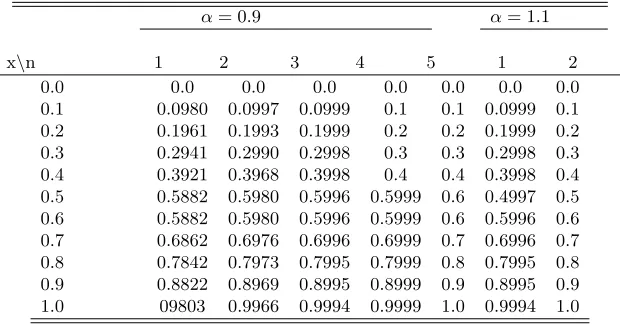
with the exact solutions φ∗(x) =x,7x. We applied Rich-type method to solve this example withα= 0.9, 1.1.The numerical results are shown in Table2. From Figure
Table 2. The values ofφn(x) in different points with different values of αfor Example 4.2
α= 0.9 α= 1.1
x\n 1 2 3 4 5 1 2
0.0 0.0 0.0 0.0 0.0 0.0 0.0 0.0 0.1 0.0980 0.0997 0.0999 0.1 0.1 0.0999 0.1 0.2 0.1961 0.1993 0.1999 0.2 0.2 0.1999 0.2 0.3 0.2941 0.2990 0.2998 0.3 0.3 0.2998 0.3 0.4 0.3921 0.3968 0.3998 0.4 0.4 0.3998 0.4 0.5 0.5882 0.5980 0.5996 0.5999 0.6 0.4997 0.5 0.6 0.5882 0.5980 0.5996 0.5999 0.6 0.5996 0.6 0.7 0.6862 0.6976 0.6996 0.6999 0.7 0.6996 0.7 0.8 0.7842 0.7973 0.7995 0.7999 0.8 0.7995 0.8 0.9 0.8822 0.8969 0.8995 0.8999 0.9 0.8995 0.9 1.0 09803 0.9966 0.9994 0.9999 1.0 0.9994 1.0
We reduced equation of Example 4.2 to a system of nonlinear algebraic equations by using Nystr¨om method with 8-point Gauss-Legedre quadrature. Then we applied Rich-type and Newton methods to solve the corresponding nonlinear system. The numerical results are listed in Table3. The stopping criterion is considered as||r||2≤
10−5,where||r||2denotes the residual norm. In this table, the initial guess has chosen
zero or random vector for Newton method and right hand side for Rich-type method. From this table, Rich-type method is relatively better than Newton method in terms of CPU time. Of course, as mentioned, Newton method has own special difficulties.
Table 3. Numerical results for Example 4.2.
Method Iteration CPU time initial guess Richardson 3 2.1403 right hand side
Newton 3 4.2639 0 Newton 3 4.4795 random
Example 4.3Consider the following system of nonlinear Fredholm integral equations
φ1(x)−λ R1
0 e
xyφ
1(y)dy−λ R1
0(x−y)φ 2
2(y)dy = f1(x),
φ2(x)−λR 1 0 e
−xyφ
1(y)dy−λR 1 0 x
2yφ2
2(y)dy = f2(x),
whereλ= 0.1, the exact solution is (φ∗1(x), φ∗2(x)) = (ex2, x) and
f1=ex
2
−λe x
2(e−1)−λ x 3 +
λ 4,
f2=x−λ
e−x
2 (e−1)−λ x2
We applied Rich-type method for solving this example withαeopt= 1.1. The numer-ical results are shown in Table4. In this table ||ri,n||∞, i= 1,2, denote the residual norm ofith component atnth iteration. As is shown from this table the convergence of Rich-type method is very fast.
Table 4. Error and residual norms for Example 4.3.
n ||e1,n||∞ ||e2,n||∞ ||r1,n||∞ ||r2,n||∞ 1 3.10e−03 1.70e−03 5.60e−03 5.70e−03 3 7.68e−06 7.57e−06 7.57e−06 7.68e−03 5 4.57e−08 2.25e−08 4.89e−08 4.80e−08 7 4.52e−10 2.51e−10 4.49e−10 4.40e−10 9 4.76e−12 2.71e−12 4.65e−12 4.57e−12
Example 4.4Consider the following system of nonlinear Fredholm integral equations
φ1(x)−λR 1
0(x+y)φ 2
1(y)dy−λ R1
0 xye
−φ2(y)dy = f 1(x),
φ2(x)−λ R1
0 e
xsin(φ
1(y))dy−λ R1
0(x
2+y2) cos(φ2
2(y))dy = f2(x),
wheref1(x) =x−λ(x3+14)+λx(2e−1−1),f2(x) =−x+λex(cos(1)−1)−λ(sin(1)x2+
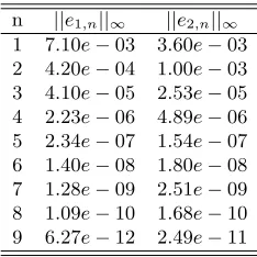
2 cos(1)−sin(1)) withλ= 0.1 and the exact solution is (φ∗1(x), φ∗2(x)) = (x,−x). We applied Rich-type method to solve this example withαeopt = 1.1 and the numerical results are given in Table5. From this table, the convergence of Rich-type method is quite impressive.
Table 5. Error norm for Example 4.4.
n ||e1,n||∞ ||e2,n||∞ 1 7.10e−03 3.60e−03 2 4.20e−04 1.00e−03 3 4.10e−05 2.53e−05 4 2.23e−06 4.89e−06 5 2.34e−07 1.54e−07 6 1.40e−08 1.80e−08 7 1.28e−09 2.51e−09 8 1.09e−10 1.68e−10 9 6.27e−12 2.49e−11
Example 4.5Consider Example 1 of [6] as follows
φ(x)−1
5 Z 1
0
cos(πx) sin(πy)φ3(y)dy= sin(πx).
The exact solution is φ∗(x) = sin(πx) + 20−
√ 391
3 cos(πx). We applied Rich-type
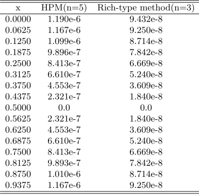
(homotopy perturbation method) of [6]. The numerical results are given in Table6for absolute solution errors in different points. From this table we see that our method converges faster than HPM.
Table 6. Numerical results for Example 4.5.
x HPM(n=5) Rich-type method(n=3) 0.0000 1.190e-6 9.432e-8 0.0625 1.167e-6 9.250e-8 0.1250 1.099e-6 8.714e-8 0.1875 9.896e-7 7.842e-8 0.2500 8.413e-7 6.669e-8 0.3125 6.610e-7 5.240e-8 0.3750 4.553e-7 3.609e-8 0.4375 2.321e-7 1.840e-8 0.5000 0.0 0.0 0.5625 2.321e-7 1.840e-8 0.6250 4.553e-7 3.609e-8 0.6875 6.610e-7 5.240e-8 0.7500 8.413e-7 6.669e-8 0.8125 9.893e-7 7.842e-8 0.8750 1.010e-6 8.714e-8 0.9375 1.167e-6 9.250e-8
Example 4.6Consider Example 1 of [4] as follows
φ(x) + Z 1
0
ex−2yφ3(y)dy=ex+1,
with the exact solutionφ∗(x) =ex. We applied Rich-type method for this example withαeopt= 0.1. The numerical results are given in Table7.
Table 7. Numerical results for Example 4.6.
x Exact solution Rich-type method(n=29) 0.1 1.105170918 1.105170918 0.2 1.221402757 1.221402758 0.3 1.349858806 1.349858807 0.4 1.491824696 1.491824697 0.5 1.648721268 1.648721270 0.6 1.822118797 1.822118800 0.7 2.013752703 2.013752707 0.8 2.225540923 2.225540928 0.9 2.459603104 2.459603111
differential equation
u00−λu0(x) +F(λ, µ, β, u(x)) = 0, x∈[0,1],
u0(0) =λu(0), u0(1) = 0,
whereF(λ, µ, β, u(x)) =λµ(β−u(x))eu(x).
The problem can be converted into a Hammerstein integral equation of the form
u(x) = Z 1
0
µk(x, t)(β−u(t))eu(t)dt, x∈[0,1],
where
k(x, t) =
1, t≤x, eλ(x−t), t > x.
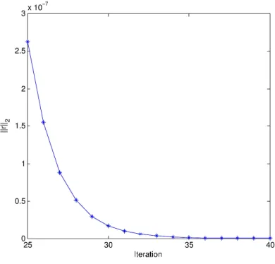
Similar to Example 4.2, we discretized equation of this example and obtained a system of nonlinear algebraic equations. Then we applied Rich-type method for the reduced algebraic system withαeopt = 1 and parameters λ= 10, µ= 0.02 and β = 3. The convergence history of this method is depicted in Figure2. The stopping criterion is considered as||r||2≤10−10,where ||r||2 denotes the residual norm of the reduced
algebraic system. This figure denotes the fast convergence of Rich-type method.
Figure 2. Convergence history of Rich-type method for Example 4.7.
Example 4.8[5] One of the great interest in hydrodynamics is the physical prob-lem
u00−eu(x)= 0, x∈[0,1],
This equation can be reformulated as the nonlinear Fredholm Hammerstein integral equation
u(x) = Z 1
0
k(x, t)eu(t)dt, x∈[0,1],
where
k(x, t) =
−t(1−x), t≤x,
−x(1−t), t > x.
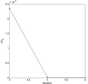
We reduced equation of this example to a system of nonlinear algebraic equations by using Nystr¨om method with 8-point Gauss-Legedre quadrature. Then we applied Rich-type method for the reduced algebraic system withαeopt= 1.5. The convergence history of this method is depicted in Figure3. For this example, the stopping criterion is considered as||r||2≤10−10,where ||r||2 denotes the residual norm of the reduced
algebraic system.
Figure 3. Convergence history of Rich-type method for Example 4.8.
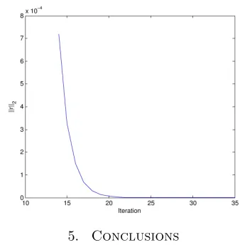
Example 4.9Consider the following nonlinear integral equation
u(x) =f(x) +λ Z 1
0
ex−tcos(u(t))dt, x∈[0,1],
whereλ= 100 and f(x) is selected so thatu(x) =x. We applied Rich-type method to solve the reduced algebraic system of this problem withαeopt= 0.1. The stopping criterion is considered as ||r||2 ≤ 10−10, where ||r||2 denotes the residual norm of
Figure 4. Convergent history of Rich-type method for Example 4.9.
5. Conclusions
In this paper, we considered a class of Hammerstein type integral equations system. We verified existence and uniqueness of solutions of these equations. We also proposed the Rich-type method to solve this type system. Convergence of the Rich-type method was analyzed and an upper bound for the error of exact solution with respect to the approximate operator was established. Some numerical experiments was presented to illustrate the efficiency of the new method.
Acknowledgment
The authors would like to thank the referees for their helpful suggestions and comments.
References
[1] H. Almasieh and M. roodaki,Triangular function method for the solution of Fredholm integral equations system,3(2012), 411-416.
[2] K.E. Atkinson,the numerical solution of integral equations of the second kind, Cambridge Univ. Press, Cambridge, 1997.
[3] E. Babolian, J. Biazar and A.R. Vahidi,The decomposition method applied to systems of Fred-holm integral equations of the second Kind, Appl. Math. Comput.,148(2004), 443-452. [4] E. Babolian and A. Shahsavaran,Numerical solution of nonlinear Fredholm integral equations
of the second kind using Haar wavelets, J. Comput. Appl. Math,225(2009), 87-95.
[5] S. Bazm,Bernoulli polynomials for the numerical solution of some classes of linear and non-linear integral equations, J. Comput. Appl. Math.,275(2015), 44-60.
[6] J. Biazar and H. Ghazvini,Numerical solution for special non-linear Fredholm integral equation by HPM, Appl. Math. Comput.,195(2008), 681-687.
[7] A. Golbabai and M. Javidi,A numerical solution for solving system of Fredholm integral equa-tions by using Homotopy Perturbation method, Appl. Math. Comput.189(2007), 1921-1928. [8] A. Golbabai and M. Javidi, Modified Homotopy Perturbation method for solving non-linear
Fredholm integral equations, Chaos. Solitons and Fractals,40(2009), 1408-1412.
[9] A. Golbabai and B. Keramati, Easy computational approach to solution of system of linear Fredholm integral equations, Chaos. Solitons and Fractals.,38(2008), 568-574.
[11] A. Jafarian and S. Measoomy Nia, Utilizing Feed-back Neural Network approach for solving linear Fredholm integral equations system, Appl. Math. Model.,37(2013), 5027-5038. [12] S. Karimi and M. Jozi,A new iterative method for solving linear Fredholm integral equations
using the least squares method, Appl. Math. and Comput.,250(2015), 744-758.
[13] K. Maleknejad, N. Aghazadeh and M. Rabbani,Numerical solution of second kind Fredholm integral equations system by using a Taylor-series expansion method, Appl. Math. comput.,175 (2006), 1229-1234.
[14] I. Moret and P. Omari,Iterative solution of integral equations by a quasi-Newton method, J. Comput. Appl. Math.,20(1987), 333-340.
[15] J. Rashidinia and M. Zarebnia,Convergence of approximate solution of system of Fredholm integral equations, J. Math. Anal. Appl.,333(2007), 1216-1227.