Please cite this article as: H. ZolfagharyAzizi, M. Naghashzadegan, V. Shokri, Comparison of the Hyperbolic Range of Two-fluid Models on Two-phase Gas-liquid Flows,International Journal of Engineering (IJE),IJE TRANSACTIONS A: Basics Vol. 31, No. 1, (January 2018) 144-156
International Journal of Engineering
J o u r n a l H o m e p a g e : w w w . i j e . i rComparison of the Hyperbolic Range of Two-fluid Models on Two-phase Gas-liquid
Flows
H. Zolfaghary Azizia, M. Naghashzadegana, V. Shokri*b
aDepartment of Mechanical Engineering, University of Guilan, Rasht, Iran
b Department of Mechanical Engineering, Sari Branch, Islamic Azad University, Sari, Iran
P A P E R I N F O
Paper history: Received 28August2017
Received in revised form 28September2017 Accepted 29October2017
Keywords: Two-Phase Flow Two-Fluid Model Numerical Simulation Hyperbolic Analysis
A B S T R A C T
In this paper, a numerical study is conducted in order to compare hyperbolic range of equations of isotherm two-fluid model governing on two-phase flow inside of pipe using conservative Shock capturing method. Differential equations of the two-fluid model are presented in two forms (i.e. form I and form II). In forms I and II, pressure correction terms are hydrodynamic and hydrostatic, respectively. In order to compare, the hyperbolic range of equations of two-fluid model is presented in two forms. One case (water Faucet Case) in the vertical configuration and two other cases (i.e. Large Relative Velocity Shock Tube Case and Toumi’s Shock Tube Case) in the horizontal configuration were used. The form I of two-fluid model had broader range of well-posing than form II of two-fluid model. The form I of two-fluid model has coefficient that proper selecting of this coefficient ensures hyperbolic roots of the characteristic equation, but in form II, roots of the characteristic equation did not have this capability.
doi: 10.5829/ije.2018.31.01a.20
1. INTRODUCTION1
In two-phase flow of gas-liquid, the gas and liquid phases are simultaneously passing through a pipeline. Due to extensive application of gas-liquid two-phase flow in various engineering problems and their more different and complex behavior than the single-phase flow; it is vital to study such flows. In addition, existence of these flows in nuclear technology and particularly in nuclear steam generators, boilers, condensers, cooling systems, as well as in gas and oil pipelines has increased the importance of studying on these two-phase flows. In two-phase flows systems, it is highly essential to exactly determine maximum range that system can work safely. In order to analyze directly two-phase flows, selecting three-dimensional Navier-Stokes equations as model has high computational cost [1]. Therefore, different models are presented in order to simplify these equations. Generally, there are three various mathematical models in order to simulate
*Corresponding Author’s Email:[email protected] (V. Shokri)
phase flow systems: Homogeneous Equilibrium Model [2], Drift Flux Model [3], and Two Fluid Model [3, 4].
in order to determine validity range of two-fluid the model. Complex roots of characteristic equation leads to an ill-posed initial value problem and failure to achieve converged and consistent results. Numerical approachs are divided into two categories in terms of pressure term: The first category of algorithms is based on pressure. Among them, Interphase Slip Algorithm [5] and Simple Algorithm can be referred [1, 6]. The second category of algorithms are algorithms based Riemann solver. Among these algorithms, Conservative Shock Capturing Method [7] and Flux Splitting Methods [8] can be referred. In this study, we focussed on this category. This category of approaches were developed form generalizing of solving methods of Shock flow to two-phase flow problems. Due to their capturing shock, these approaches are used in order to predict discontinuities in the interface of two phase flows. The second category of algorithms are considered as explicit numerical schemes. In order to calculate time step, they are dependent on maximum value of wave velocity. The maximum value of wave velocity for two-fluid model is equal to maximum value of the roots of the characteristic equation of governing equations in solution field. Derivative by varying the terms of the two-fluid model, which generally are related to assumptions of pressure and pressure correction terms, the two-fluid model requires to new hyperbolic analysis and determining real roots of the characteristic equation. In the two-fluid model, there is a difference between pressure of each phase and pressure of the same phase at the interface. The pressure difference between pressure of each phase and pressure of the same phase at the interface is called “term correction pressure”.
In order to determine the roots of the characteristic equation, they performed hyperbolic analysis of two-fluid model using density perturbation method and obtained the approximate values of the roots of the characteristic equation for the two-fluid model equations governing the solution field. After them, other researchers used these assumptions of pressure and the roots of the characteristic equation presented to numerically model of two-phase flows in various fields [9-11].
Issa and Kempf [1] used the two-fluid model in order to Simulation of slug flow in horizontal and nearly horizontal pipes with the two-fluid model.
In order to solve two-fluid equations governing on the solution field, Issa and Kempf [1] used a Staggered mesh using finite volume numerical method. Because of this numerical method is unconditional stable, there is no sensitivity to find the roots of the characteristic equation. Therefore, for calculating time step, they considered characteristic value as the maximum velocity of the gas (𝜆𝑛𝑚𝑎𝑥= 𝑢𝑔,𝑚𝑎𝑥𝑛 ). Also, they considered value of Courant Friedrichs Levy Number equal to 0.5. After them, other researchers used these assumptions of
pressure and the roots of the characteristic equation in order to numerical modeling of two-phase flows in various fields [6, 12-14]. Omgba-Essama [2], used fluid model in order to numerical modelling of two-phase flows. In this two-fluid model, assumptions of pressure and pressure correction term presented by Issa and Kempf [1] were used. In this study, numerical modelling was performed through Flux Splitting Methods that is based on Riemann solver. In this study, it was stated that obtaining the roots of the characteristic equation through accurate analytical method is very difficult. Therefore, four real characteristic values for the roots of the characteristic equation was presented using the perturbation method around a small parameter. It should be noted that eigenvalues obtained using approximate method are valid only for a small perturbations and it ensures governing hyperbolic two-fluid equations.
Hanyang and Liejin [15] used a transient two-fluid model in order to evaluate the interfacial instability and the initiation of slug regime in gas-liquid two-phase flows at the horizontal channel.
They used a staggered mesh based on the finite volume method in order to calculate pressure term. Also, they used maximum velocity of the gas phase in each time step and set Courant Friedrichs Levy Number equal to 0.5.
Figueiredo et al. [16] investigated accuracy of the Flux-Corrected Transport numerical method applied to transient two-phase flow simulations in gas pipelines. The governing equation presented are based on pressure assumptions presented by Issa and Kempf [1]. In
Numerical analysis, they used the maximum
characteristic value presented by Omgba-Essama [2]. Bueno et al. [17] perform numerical simulation of stratified Two-Phase Flow in a Nearly Horizontal Gas-Liquid Pipeline With a Leak. In their research, they used pressure assumptions presented by Issa and Kempf [1]. Also, they used the roots of characteristic equation presented by Omgba-Essama [2].
According to literature, it was found that two models (i.e. hydrostatic model and hydrodynamic model) were used to express pressure correction term for simulating gas-liquid two-phase flows using two-fluid model. The use of each of these models requires a unique hyperbolic analysis and determination of the roots of the characteristic equation for each of the models. The roots of the characteristic equation affect directly both on the nature of mathematical models and accuracy of numerical algorithms of the solution. The roots of the characteristic equation for hydrodynamic model are presented by Evje and Flåtten [8]. Furthermore, the roots of the characteristic equation for hydrostatic model are presented by Essama [2].
Therefore, in the present paper, effects of the roots of the characteristic equation on the hyperbolic range of the two-fluid model were investigated by choosing three valid cases of two-phase flow (i.e. water faucet case, large relative velocity shock tube case, and Toumi’s shock tube case) with different initial conditions for the variables of flow (i.e. velocity, volume fraction of phases, and pressure).
2. GOVERNING EQUATIONS
The spatial average form of two-fluid model is very practical for complex engineering applications. Averaged two-fluid model is obtained from integrating three-dimensional two-fluid model in terms of position on the cross-section and using suitable average values [3]. Momentum and energy transferred between each phase and the wall, as well as dynamic interaction between phases at the interface appear source terms and empirical relations are used to calculate them [4].
The average form of two-fluid model equations governing on the solution field is demonstrated as following [8]. In this study, the flow is considered as isotherm. Conservation of mass and momentum equations for gas and liquid phases are stated as follows:
Mass conservation equation for gas:
𝜕
𝜕𝑡(𝜌𝑔𝑅𝑔) + 𝜕
𝜕𝑥(𝜌𝑔𝑅𝑔𝑢𝑔) = 0 (1)
Mass conservation equation for liquid:
𝜕
𝜕𝑡(𝜌𝑙𝑅𝑙) + 𝜕
𝜕𝑥(𝜌𝑙𝑅𝑙𝑢𝑙) = 0 (2)
Momentum conservation equation for gas:
𝜕
𝜕𝑡(𝜌𝑔𝑅𝑔𝑢𝑔) + 𝜕
𝜕𝑥(𝜌𝑔𝑅𝑔𝑢𝑔
2) = −𝜕
𝜕𝑥
((𝑃𝑔− 𝑃𝑔𝑖)𝑅𝑔) − 𝑅𝑔
𝜕𝑃𝑔𝑖
𝜕𝑥 −𝜌𝑔𝑅𝑔𝐺𝑠𝑖𝑛𝛽 + 𝐹𝑔𝑤+ 𝐹𝐼
(3)
Momentum conservation equation for liquid:
𝜕
𝜕𝑡(𝜌𝑙𝑅𝑙𝑢𝑙) + 𝜕 𝜕𝑥(𝜌𝑙𝑅𝑙𝑢𝑙
2) = −𝜕
𝜕𝑥
((𝑃𝑙− 𝑃𝑙𝑖)𝑅𝑙) − 𝑅𝑙
𝜕𝑃𝑙𝑖
𝜕𝑥−𝜌𝑙𝑅𝑙𝐺𝑠𝑖𝑛𝛽 + 𝐹𝑙𝑤− 𝐹𝐼
(4)
where, for kth phase, (if 𝑘 = 𝑔, then the phase is gas and if 𝑘 = 𝑙, then the phase is liquid). Also,𝜌𝑘,𝑢𝑘,𝑃𝑘, and 𝑃𝑘𝑖 are density in kth phase, volume fraction in kth phase, velocity in kth phase, pressure in kth phase, and pressure at the interface in kth phase, respectively. (𝜌𝑘𝑅𝑘𝐺𝑠𝑖𝑛𝛽), 𝐹𝑘𝑤, and 𝐹𝐼 are gravitational force term, friction force of each phase with the walls, and friction force of phases at the interface, respectively. G is the acceleration of gravity.
In above momentum equations, the term 𝑃𝑔− 𝑃𝑔𝑖 is indicated as ∆𝑃𝑔𝑖 and called “pressure correction term
for the gas phase”. Also, the term 𝑃𝑙− 𝑃𝑙𝑖 is indicated as ∆𝑃𝑙𝑖 and called “pressure correction term for the liquid phase”. Pressure terms in above momentum equations can be expressed as two forms in terms of the extension of the derivative to variables.
− 𝜕
𝜕𝑥((𝑃𝑘− 𝑃𝑘𝑖)𝑅𝑘) − 𝑅𝑘
𝜕𝑃𝑘𝑖
𝜕𝑥 (5)
= −𝜕(𝑅𝑘𝑃𝑘)
𝜕𝑥 + 𝑃𝑘𝑖
𝜕𝑅𝑘
𝜕𝑥 (6)
= −𝑅𝑘𝜕𝑃𝜕𝑥𝑘− 𝛥𝑃𝑘𝑖𝜕𝑅𝜕𝑥𝑘 (7)
Now, different forms of two-fluid model are obtained by applying different assumptions for the pressure term. Evje and Flåtten [8], used Equation (5) for pressure terms and assumed that the pressure of gas phase is equal to the pressure of liquid phase (𝑃𝑔= 𝑃𝑙= 𝑃) as well as the pressure of phases at the interface (𝑃𝑔𝑖= 𝑃𝑙𝑖 = 𝑃𝑖), and in order to correct pressure, the following relation was used:
∆𝑃𝑘𝑖= 𝑃𝑘− 𝑃𝑘𝑖= 𝛿
𝑅𝑙𝑅𝑔𝜌𝑙𝜌𝑔
𝜌𝑔𝑅𝑙+𝜌𝑙𝑅𝑔(𝑢𝑔− 𝑢𝑙)
2
(8)
In this paper, the Equations (1) - (4) and (8) is called the equations form I. Issa and Kempf presented the following relations for the pressure term of two-fluid model by considering the Equation (6) and hydrostatic pressure assumption for liquid phase and calculating the average pressure of the liquid phase by integrating of the cross-section of the pipe [1]:
− 𝜕
𝜕𝑥((𝑃𝑔− 𝑃𝑔𝑖)𝑅𝑔) − 𝑅𝑔
𝜕𝑃𝑔𝑖
𝜕𝑥 = −𝑅𝑔
𝜕𝑃
𝜕𝑥 (9)
In their work, it was assumed that the gas phase pressure is equal to the gas phase pressure at the interface (i.e. (Pg= Pgi= P)).
−𝜕𝑥𝜕((𝑃𝑙− 𝑃𝑙𝑖)𝑅𝑙) − 𝑅𝑙𝜕𝑃𝜕𝑥𝑙𝑖= n − 𝑅𝑙𝜕𝑃𝜕𝑥−
𝜌𝑙𝑅𝑙𝐺 𝑐𝑜𝑠 𝛽
𝜕ℎ𝑙
𝜕𝑥
(10)
ℎ𝑙 is height of the liquid phase. Also, it was assumed that the liquid phase pressure at the interface is equal to the gas phase pressure at the interface (i.e. (𝑃𝑔𝑖= 𝑃𝑙𝑖= 𝑃)). In addition, the liquid phase pressure varies hydrostatically in direction of vertical axis. Also, in some references [2], Equation (7) was used for the term pressure of momentum equation. The following relation was presented the pressure correction term:
𝑃𝑐= ∆𝑃𝑘𝑖= 𝜌𝑙𝑅𝑙𝐺 𝑐𝑜𝑠 𝛽𝜕ℎ𝜕𝑅𝑙
𝑙 (11)
By replacing Equation (11) into Equation (7), we have:
−𝑅𝑘
𝜕𝑃𝑘
𝜕𝑥 − 𝜌𝑙𝑅𝑙𝐺 𝑐𝑜𝑠 𝛽
𝜕ℎ𝑙
𝜕𝑅𝑙
𝜕𝑅𝑙
𝜕𝑥= −𝑅𝑘
𝜕𝑃𝑘
𝜕𝑥 −
𝜌𝑙𝑅𝑙𝐺 𝑐𝑜𝑠 𝛽
𝜕ℎ𝑙
𝜕𝑥
where, the Equation (12) is the same Equation (10). Equations (1)-(4) and (10) is called the equations form II. For completing the system of equations, additional relations are required. These relations, a geometric constraint and the relationship between density and pressure of phases are included. A geometric constraint states that summation of volume fractions of the two phases [2]:
𝑅𝐿+ 𝑅𝐺= 1 (13)
The relationship between density and pressure of phases are presented stated as follows [8]:
𝜕𝑃𝑘
𝜕𝜌𝑘= 𝐶𝑘 2
(14)
where, Ck is the speed of sound in each phase.
Cg2= 105(m s⁄ )2 Cl2= 106(m s⁄ )2
3. HYPERBOLIC ANALYSIS EQUATIONS
3. 1. Hyperbolic Analysis of Form I The basic
governing equations are presented as quasi-linear. This form of a governing equation are required in order to express eigenvalues and hyperbolic analysis of the fluid model. In fact, the governing equations on two-fluid model must be written as below:
𝜕𝑄
𝜕𝑡+ 𝐴(𝑄)
𝜕𝑄
𝜕𝑥= 𝑆(𝑄) (15)
In above relation, 𝑄, 𝑆, and 𝐴(𝑄) are conservative variables vector, vector including source term, and system’s matrix, respectively. The vectors Q and S, and the matrix 𝐴 for two-fluid model are defined as following:
𝑄 = [𝑅𝑔𝜌𝑔𝑅𝑙𝜌𝑙𝑅𝑔𝜌𝑔𝑢𝑔𝑅𝑙𝜌𝑙𝑢𝑙]
𝑇
(16)
𝑆 = [ 0 𝑅𝑔𝜌𝑔𝐺 0 𝑅𝑙𝜌𝑙𝐺]
𝑇
(17)
𝐴 =
[
0 0 1
0 0 0
𝐴31 𝐴32 2𝑢𝑔
0 1 0
𝐴41 𝐴420 2𝑢𝑙]
(18)
𝐴31=
𝑅𝑔𝜌𝑙+∆𝑃𝑔𝑖𝑅𝑙𝐶𝑙2
𝑘 − 𝑢𝑔
2 (19-1)
𝐴32=
𝑅𝑔𝜌𝑔+∆𝑃𝑔𝑖𝑅𝑔𝐶𝑔2
𝑘
(19-2)
𝐴41=
𝑅𝑙𝜌𝑙+∆𝑃𝑙𝑖𝑅𝑙𝐶𝑙2
𝑘
(19-3)
𝐴42=
𝑅𝑙𝜌𝑔+∆𝑃𝑙𝑖𝑅𝑔 𝐶𝑔2
𝑘 − 𝑢𝑙
2 (19-4)
where, 𝑘 = 𝑅𝑙𝜌𝑔⁄𝐶𝑙2+ 𝑅𝑔𝜌𝑙⁄𝐶𝑔2. The range in which the two-fluid model equations remains as hyperbolic can be determined by calculating eigenvalues of the matrix I. Because of the complexity of the desired matrix characteristic equation, there is no exact analytical equation to calculate the eigenvalues of matrix. Using analysis of density perturbations of the equation (20) for the eigenvalues of the matrix I, Evje and Flatten[8] demonstrated that the Equations (21)-(24) are valid.
𝜆{1,2}= 𝑢𝑃± 𝐶𝑚 , 𝜆{3,4}= 𝑢𝑢± 𝑣 (20)
𝑢𝑃=
𝑅𝑔𝜌𝑙𝑢𝑔+𝑅𝑙𝜌𝑔𝑢𝑙
𝑅𝑔𝜌𝑙+𝑅𝑙𝜌𝑔 (21)
𝑢𝑢=
𝑅𝑔𝜌𝑙𝑢𝑙+𝑅𝑙𝜌𝑔𝑢𝑔
𝑅𝑔𝜌𝑙+𝑅𝑙𝜌𝑔 (22)
𝑣 = √𝛥𝑃𝑖(𝑅𝑔𝜌𝑙+𝑅𝑙𝜌𝑔)−𝑅𝑔𝑅𝑙𝜌𝑙𝜌𝑔(𝑢𝑔−𝑢𝑙)2
(𝑅𝑔𝜌𝑙+𝑅𝑙𝜌𝑔)2
(23)
𝐶𝑚= √
𝑅𝑔𝜌𝑙+𝑅𝑙𝜌𝑔
(𝜕𝜌𝑔𝜕𝑃)𝑅𝑔𝜌𝑙+(𝜕𝜌𝑙𝜕𝑃)𝑅𝑙𝜌𝑔
(24)
The Equation (23) shows that if 𝛥𝑃𝑖= 0, then eigenvalues are complex. Thus, In Equation (8), δ must be more than one.
with 𝛿 a positive constant. Taking 𝛿 ≥ 1makes the two-fluid model hyperbolic [8]. If the initial velocities of phases are equal, according to Equation (8), the pressure correction term is zero which means that 𝑃𝑘 is equal to 𝑃𝑘𝑖. In this case, the system of governing equations has complex eigenvalues, resulting an ill-posed initial value problem, where there is an unphysical and unbounded growth of small wavelength of disturbances [8].
3. 2. Hyperbolic Analysis of Form II In order to
determine the eigenvalues of the system, first, systems of a governing equation are written as the following compact form:
𝑀𝐴
𝜕𝜓
𝜕𝑡 + 𝑀𝐵
𝜕𝜓
𝜕𝑥= 𝑆 (25)
𝑑𝑒𝑡(𝑀𝐵− 𝜆𝑀𝐴) = 0 (26)
where, λ is a characteristic value. Equation of form II can be written as Equation (25) and using the
following matrix [2].
𝑀𝐴=
[
−𝜌𝑔 0 0
1 0 0
0 𝜌𝑔𝑅𝑔 0
𝑅𝑔
0 0
0 0𝜌𝑙𝑅𝑙 0 ]
(27)
𝑀𝐵=
[
−𝜌𝑔𝑢𝑔 𝜌𝑔𝑅𝑔 0
𝑢𝑙 0 𝑅𝑙
0 𝜌𝑔𝑅𝑔𝑢𝑔 0
𝑅𝑔𝑢𝑔
0
𝑅𝑔𝐶𝑔2
𝑃𝐶 0 𝜌𝑙𝑅𝑙𝑢𝑙 𝑅𝑙𝐶𝑔2]
(28)
where,Cg2= ∂P ∂ρ⁄ g is the square of the speed of sound of gas. By replacing matrices (27) and (28) in Equation (26), characteristic polynomial is obtained as below:
−𝜆̃4+ 𝜆̃2(1 + 𝜒 + 𝑃̂) − 𝑃̂ + 2𝜃𝜆̃(1 − 𝜆̃2) + 𝜃2(1 −
𝜆̃2) = 0 (29)
where,
𝜆̃ =𝜆−𝑢𝑔
𝐶𝑔 (30)
𝑃̂ = 𝑃𝐶
𝜌𝑙𝐶𝑔2=
𝐴𝑙𝐺 𝑐𝑜𝑠 𝛽
𝑑𝐴𝑙/𝑑ℎ𝑙𝐶𝑔2 (31)
𝜃 =𝑢𝑟
𝐶𝑔=
𝑢𝑔−𝑢𝑙
𝐶𝑔 (32)
Perturbation method about the small parameter θ = ur⁄Cg is used. For the majority of flows that exist in the pipeline, the relative velocity 𝑢𝑟 has order of several meters per second. Also, the speed of sound in the gas is order of 200 to 300 meters per second. Therefore, parameter θ is small and it seems that this parameter for perturbation analysis is suitable [2]. Using Goursat's lemma, we have: Where P(x, θ) is in terms of small parameter θ and the real coefficient x:
𝑃(𝑥, 𝜃) = 𝑃0(𝑥) + 𝜃𝑃1(𝑥) +
𝜃2
2𝑃2(𝑥) (33)
Where, 𝑃0(𝑥),𝑃1(𝑥), and 𝑃2(𝑥)are polynomial having three terms with real coefficients. The purpose is to find roots of the polynomial 𝑃(𝑥, 𝜃) having real coefficientsin neighboring of root of the polynomial 𝑃0(𝑥) (i.e.x0). There may be two cases. In the first case 𝑥0 is unit root of the polynomial 𝑃0(𝑥) and in the second case, P0(x) has two roots. In this paper, the first case occurs. If the 𝑥0 is unit root of the polynomial 𝑃0(𝑥), then there is a first order function𝑥(𝜃) that is differentiable in terms 𝜃 so that 𝑃(𝑥(𝜃), 𝜃) = 0 and we have:
𝑃0 ́ is first derivative of the polynomial 𝑃0(𝑥). by combining Equations (29) and (33), the following polynomials are obtained:
{
𝑃0(𝜆̃) = −𝜆̃4+ 𝜆̃2(1 + 𝜒 + 𝑃̂) − 𝑃̂
𝑃1(𝜆̃) = 2𝜆̃(1 − 𝜆̃2)
𝑃2(𝜆̃) = 2(1 − 𝜆̃2)
(34)
𝑥(𝜃) = 𝑥0+ 𝜃𝑧1+ 𝑂(𝜃) (35)
𝑧1= −
𝑃1(𝑥0)
𝑃0′(𝑥0) (36)
To obtain zeros of the polynomial P0(λ̃), it is sufficient to solve the following equation:
−𝜆̃4+ 𝜆̃2(1 + 𝜒 + 𝑃̂) − 𝑃̂ = 0𝜆̃→ 𝑦2=𝑦 2− 𝑦 (1 + 𝜒 +
𝑃̂) + 𝑃̂ = 0
(37)
To obtain the roots of the equation (37), we write:
𝛥𝑆= (𝜒 + (1 − √𝑃̂)2) . (𝜒 + (1 + √𝑃̂)2) (38)
We always have: ∆S≥ 0 → P̂ ≥ 0 ⟹ cos β ≥ 0 Two roots of the equation are:
{y
+=(1+χ+P̂)+√∆S 2
y−=(1+χ+P̂)−√∆S 2
(39)
The root of y+ is positive because of all of its terms are positive. Also, it can be proved through the limit of minimum that 𝑦− is positive.
𝑦−≥ 𝑦−
𝑚𝑖𝑛=
(1+𝜒+𝑃̂)−√𝛥𝑚𝑎𝑥𝑆
2
(40)
and
𝛥 = (1 + 𝜒 + 𝑃̂)2− 4𝑃̂ < (1 + 𝜒 + 𝑃̂)2= 𝛥𝑚𝑎𝑥𝑆 (41)
also
𝑦−≥ 𝑦−
𝑚𝑖𝑛= 0 ⟹ 𝑦−≥ 0 (42)
Therefore, both roots are positive. Characteristic values of Equation (37) are obtained, stated as follows:
{
𝜆̃1= −√𝑦+
𝜆̃2= −√𝑦−
𝜆̃3= √𝑦−
𝜆̃4= √𝑦+
(43)
Using Equations (35) and(36), we have:
{𝑧1,4=
1−𝑦+
2𝑦+−(1+𝜒+𝑃̂)
𝑧2,3= 1−𝑦
−
2𝑦−−(1+𝜒+𝑃̂)
(44)
{
𝜆1= 𝑢𝑔− 𝐶𝑔√𝑦++ 𝑢𝑟
1−𝑦+
2𝑦+−(1+𝜒+𝑃̂ )
𝜆2= 𝑢𝑔− 𝐶𝑔√𝑦−+ 𝑢𝑟 1−𝑦
−
2𝑦−−(1+𝜒+𝑃̂ )
𝜆3= 𝑢𝑔+ 𝐶𝑔√𝑦−+ 𝑢𝑟
1−𝑦−
2𝑦−−(1+𝜒+𝑃̂ )
𝜆4= 𝑢𝑔+ 𝐶𝑔√𝑦++ 𝑢𝑟
1−𝑦+
2𝑦+−(1+𝜒+𝑃̂ )
(45)
where,
𝜒 =𝜌𝑔𝑅𝑙
𝜌𝑙𝑅𝑔 (46)
𝑃̂ =𝐴𝑙𝐺 𝑐𝑜𝑠 𝛽
𝐴𝑙′ (47)
𝐴𝑙′=𝑑𝐴𝑙
𝑑ℎ𝑙 (48)
𝑢𝑟= 𝑢𝑔− 𝑢𝑙 (49)
𝑢𝑟 is the relative velocity of phases. Two-phase flow models are highly sensitive to being real or imagine of their roots of characteristic equation. If the roots of characteristic equation of differential equations governing on model are imagine, then an ill-posed initial value problem is formed, as result, unlimited instabilities are occurred and eventually the results cannot be convergent. But if the roots of characteristic equation are real, then well-posed initial value problem is formed unlimited instabilities are removed [18]. The limit of stability of two-fluid model by considering the hydrostatic pressure correction term is the Kelvin Helmholtz instability that is obtained expressed as follows [2].
(𝑢𝑔− 𝑢𝑙)
2
≤ √(𝑅𝑔𝜌𝑙+ 𝑅𝑙𝜌𝑔)
𝜌𝑙−𝜌𝑔
𝜌𝑙𝜌𝑔 𝑔 𝑐𝑜𝑠 𝛽
𝐴
𝜕𝐴𝑙 𝜕ℎ
(50)
It means that the limit of Kelvin Helmholtz instability is equal to limit of well-posing of a single-pressure two-fluid model by considering the hydrostatic pressure correction term. On the one hand it can be shown that if the velocity difference between the two phases is more than this value, then the interface between the two phases are physically unstable as well. It means that limit of physical instability at the interface is equal to well-posing of single-pressure two-fluid model by considering the hydrostatic pressure correction term . If the velocity difference between the two phases is more than this value, then the roots of characteristic equation is imagine and the model is ill-posed. This ill-posing causes that the results do not show realistic physics of two-fluid flow model.
4. NUMERICAL SOLUTION METHODS
Single-pressure two-fluid model equations can be written as non- conservative, as following [7]:
𝜕𝑄 𝜕𝑡+
𝜕𝐹
𝜕𝑥= 𝐻
𝜕𝑅𝑘
𝜕𝑥 + 𝑆 (51)
Q is conservative variables vector. F is conservative flux vector. Also, 𝑆 and 𝐻 𝜕𝑅𝑘⁄𝜕𝑥 are transfer vectors of the interface and are included all non-conservative terms. For non-conservative system Equation (51) form of the discretization equation is as following [7]:
𝑄𝑖𝑛+1= 𝑄𝑖𝑛+
∆𝑡 ∆𝑥(𝐹𝑖−1/2
𝑛 − 𝐹
𝑖+1/2𝑛 ) + ∆𝑡 (𝐻 𝜕𝑅𝑘
𝜕𝑥) +
∆𝑡𝑆𝑖
(52)
In Equation (52), n and 𝑛 + 1 denotes the old and new time steps respectively. Also 𝑖 represents the cell. To calculate the numerical flux term 𝐹𝑖+1/2𝑛 , lax-friedrichs method is used.
4. 1. Lax-Friedrichs Method In this method, flux
is calculated as following [7]:
𝐹𝑖+1 2𝑛𝐿𝐹⁄ = 1 2(𝐹𝑖+1
𝑛 + 𝐹
𝑖𝑛) −
∆𝑥 2∆𝑡(𝑄𝑖+1
𝑛 − 𝑄
𝑖𝑛) (53)
Numerical flux in the cell ith is defined as 𝐹𝑖𝑛= 𝐹(𝑄𝑖𝑛) that is obtained based on the physical flux term expressed by the model. Single- equations two-fluid model pressure have the non-conservative terms 𝐻 𝜕𝑅𝑘⁄𝜕𝑥 that must be separated properly. Otherwise, this term causes instability in the results [19].
In order to discrete the non-conservative term 𝐻 ∂Rk⁄∂x, the following equations are presented [19]:
𝐻𝜕𝑅𝜕𝑥𝑔= 𝐻𝑅𝑔𝑅𝑙𝜕𝐵𝐺𝜕𝑥 (54)
𝐻𝜕𝑅𝑙
𝜕𝑥= 𝐻𝑅𝑙𝑅𝑔 𝜕𝐵𝐿
𝜕𝑥 (55)
The derivative terms 𝜕𝐵𝐺 𝜕𝑥⁄ and 𝜕𝐵𝐿 𝜕𝑥⁄ are separated using the central scheme [19]:
𝐻𝑅𝑔𝑅𝑙
𝜕𝐵𝐺
𝜕𝑥 = 𝐻𝑅𝑔𝑅𝑙
𝐵𝐺𝑖+1−𝐵𝐺𝑖−1
2∆𝑥 (56)
𝐻𝑅𝑙𝑅𝑔𝜕𝐵𝐿𝜕𝑥 = 𝐻𝑅𝑔𝑅𝑙𝐵𝐿𝑖+12∆𝑥−𝐵𝐿𝑖−1 (57)
where [19]
𝐵𝐺 = 𝑙𝑜𝑔 (𝑅𝑔
𝑅𝑙) (58)
𝐵𝐿 = 𝑙𝑜𝑔 (𝑅𝑙
𝑅𝑔) (59)
4. 2. Calculation Time Step In order to calculate
time step, first, ∆𝑥 is considered as mesh size, then the time step ∆𝑡 is calculated using the following realation [2].
∆𝑡 = 𝐶𝐹𝐿 ∆𝑥
𝜆𝑚𝑎𝑥𝑛
(60)
𝜆𝑚𝑎𝑥𝑛 is the maximum value of the wave velocity on the solution field at the time of 𝑛. The maximum value of wave velocity for the single-pressure two-fluid model is equal to the maximum value of the characteristic equation a governing on the solution field. The characteristic value of the two-fluid model was presented by Omgba-Essama [2] by considering the term hydrostatic pressure the correction. Also, the characteristic value of the two-fluid model was presented by Evje and Flåtten [8] by considering the term hydrodynamic pressure the correction.
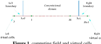
4. 3. Boundary Condition For a computing domain (0, L) discretized into M computing cells of length ∆𝑥, we require special conditions at the boundary positions x=0 and x=L as illustrated in Figure 1. These boundary conditions are expected to provide for test case the numerical fluxes 𝐹1/2𝑛𝐿𝐹and 𝐹𝑀+1/2𝑛𝐿𝐹 , which are required by finite difference discretisation such as Equation (53) in order to advance the extreme cells 1 and M to the next time level. For this, in the input and output, virtual grid will be considered and zeroth-order extrapolation for the virtual points are used for the flux in entry and outlet.
5. VALIDATION OF METHODS
In this section, in order to observe the effect the roots of the characteristic equation on the accuracy of the results, three case studies namely water faucet case, large relative velocity shock tube case, and Toumi’s shock tube case are analyzed using two-fluid model.
5. 1. Water Faucet Case This system is comprised
of a vertical pipe have a height of 12 meters and a diameter of 1 m. At the initial moment, velocity of water is 10 𝑚 𝑠⁄ and velocity of water is 0, and the volume fraction of water is assumed 0.8. The pressure in the channel is equal to 100000 Pa. Inlet conditions is equivalent to the initial conditions and for outlet of pipe, fully developed boundary condition are valid. Around the water, the air having density of 1.16 𝑘𝑔 𝑚⁄ 3 flows continuously, also the density of water is considered 1000 𝑘𝑔 𝑚⁄ 3[2]. Figure 2 shows schematic of water faucet case.
Figure 1. computing field and virtual cells
Figure 2. Schematic of water faucet case
In water faucet case, pressure inlet condition, velocity outlet, and fully developed are used for pressure boundary conditions in inlet, velocity term in outlet, and void fraction, respectively.
Analytic solution of water faucet case is presented in the reference [20]. Results of the reference were extracted from Evje and Flåtten [20].
First, independent results of computing mesh for volume fraction profile of the gas-phase of both forms presented were obtained for the roots of the characteristic equation. Figures 3 and 4 indicate dependency of results computational mesh for volume fraction profile of the gas-phase at the time 0.6s for 𝐶𝐹𝐿 = 0.5.
The independent result of the computational mesh for volume fraction profile of the gas-phase is shown in the above stated figures, respectively, using the root of the characteristic equation of form II and root of the characteristic equation of form I. It was found that in the computational mesh 6400, results are independent on the computational mesh.
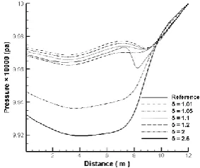
Figure 5 shows the effect of value of δ on calculating the roots of the characteristic equation of form I as well as direct effect of value of δ effect on accuracy of prediction of pressure changes profile. Figure 6 compares accuracy of the roots of the characteristic equation of form I and form II, in where 𝛿=1.2. The number of computational mesh is 6400. Also, calculations time and the Courante-Friedrichs-Levy number are equal to 0.6 and 0.5, respectively.
Figure 3. Water Faucet Case. volume fraction profile of the
Figure 4. Water Faucet Case. volume fraction profile of the gas-phase for the roots of the characteristic equation of form (I)
Figure 5. Water Faucet Case. Comparison of different values
of δ for root of the characteristic equation of form (I) for the pressure changes profile
Figure 6. Water Faucet Case. Comparison of root of the
characteristic equation forms (I) and (II) for the pressure changes profile
The results of pressure changes profile presented in the Figure 6 show that results obtained for the pressure changes profile using the roots of the characteristic equation of form I have better agreement with the analytical solution of the water faucet case . Hydrostatic pressure correction term for the water faucet case is equal to zero because channel is vertical and cos 𝛽 in Equation (10) is zero. As a result, the effect of hydrostatic pressure correction term in the two-fluid equations is removed. In fact, we assumed 𝑃𝑖𝑙 = 𝑃𝑖𝑔=
𝑃𝑙= 𝑃𝑔= 𝑃. This causes that the roots of characteristic equation, unconditionally to be complex. And in this case, use of form is no suggested. Therefore, there is the mismatch of results obtained while using the roots of the characteristic equation of form II to analytical solution of water faucet case.
In numerical modeling, we assumed that(𝑃𝑔= 𝑃𝑙). The gas phase pressure is calculated according to Equation (14). The pressure changes profile predicted by the roots of the characteristic equation of form II has a greater increase than pressure changes profile predicted by the roots of the characteristic equation of form I. According to Figure 9, the gas phase volume fraction profile predicted by the roots of the characteristic equation of form II has grown more than the proportions of the gas phase predicted by the roots of the characteristic equation of form I.Therefore, the further growth of the gas-phase volume fraction profile predicted by the roots of the characteristic equation of form II increases cross-section of the gas phase.
According to Bernoulli's equations, increases in cross-section of the gas phase leads to increase in pressure, increase in liquid phase velocity and in decrease in gas phase velocity. Results of pressure changes profile, gas phase velocity profile and liquid phase velocity are indicated in Figures 6, 7 and 8, respectively. Mathematically, the gas phase velocity profile, the liquid phase velocity profile and the volume fraction profile of the gas phase are investigated.
Velocity changes profile of the gas phase in Figure 7 shows that the roots of the characteristic equation of form I, by considering the most unfavorable value of δ, are presented more accurate results than the roots of the characteristic equation of form II.
Also, results of the gas-phase volume fraction profile and liquid phase velocity in Figures 9 and 8 show more consistent the results of roots of the characteristic equation of form II.
Figure 7.Water faucet case. Comparison of effect of the roots
Figure 8.Water faucet case. Comparison of effect of the roots of the characteristic equation of forms (I) and (II) for velocity profile of the liquid phase
Figure 9.Water faucet case. Comparison of effect of the roots
of the characteristic equation of forms (I) and (II) for volume fraction profile of the gas-phase
This contradiction is not caused by the impact of the roots of the characteristic equation, but it is caused by ill-posing of the two-fluid model having hydrostatic pressure correction term.
By considering hydrostatic pressure correction term, because of Kelvin Helmholtz instability is equal to the limit of well-posing of two-fluid model [2]. Therefore, due to being vertical of pipe, the cos 𝛽 in the Equation (10) is zero. As a result, the left side of Kelvin Helmholtz instability of the Equation (50) is zero and we have (𝑢𝑔− 𝑢𝑙)
2
≤ 0. But, according to the initial velocity of the two phases, this condition is not valid for the water faucet case. Therefore, the water faucet case is an ill-posed initial value problem that validation of results is possible by comparing the analytical solution of the problem.
5. 2. Large Relative Velocity Case This problem is a Riemann initial value problem that is included a channel with 100 m length that in position of 50 m are divided in two parts and both ends of the channel are closed. Characteristics of this problem and initial conditions on the left and right diaphragm are presented
in Table 1 [21]. Schematic of large relative velocity case is shown in Figure 10.
Figures 11 and 12, dependency on computational mesh solutions for the velocity profile of the gas phase at the time of 0.1 seconds for the CFL = 0.5 are shown. These figures indicate the results independent on the computational mesh for velocity profile of the gas phase using the roots of the characteristic equation of form I and the roots of the characteristic equation of form II, respectively. It was found that in the computational
mesh 1600, results are independent on the
computational mesh.
In this section, we compared the roots of the characteristic equation of form I and form II. The results presented for pressure changes profile, volume fraction profile of the liquid phase, velocity profile the of gas phase and velocity profile of the liquid phase in Figures 13-16, respectively are valid.
Results of pressure changes profile are shown in Figure 13. The most appropriate amount of δ for the roots of the characteristic equation of form I, that ensures being well-posed of the model and compliance with analytical solutions, is 1.2.
Figure 10. Schematic of large relative velocity case
TABLE 1. Initial conditions of the large relative velocity
shock tube case
Quantity Unit Left Right
Gas volume fraction - 0.29 0.3
Liquid velocity 𝑚 𝑠⁄ 1 1
Gas velocity 𝑚 𝑠⁄ 65 50
Pressure 𝐾𝑝𝑎 265 265
Gas density 𝑘𝑔 𝑚⁄ 3 2.65 2.65 liquid density 𝑘𝑔 𝑚⁄ 3 1000 1000
Figure 11. Large relative velocity shock tube case. velocity
Figure 12. Large relative velocity shock tube case. velocity profile of the gas phase of the roots of characteristic equation of form (I)
Figure 13. Large relative velocity case. Comparison of the
effects of the roots of the characteristic equation of forms (I) and (II) for pressure changes profile
Figure 14. Large relative velocity case. Comparison of the
effects of the roots of the characteristic equation of forms (I) and (II) for the volume fraction profile of the liquid phase.
The values of 2 and 2.5 for δ causes being ill-posed of the model and leads to incorrect prediction for solving wave motion, in fact, it shows misinformation from the actual physics of flow.
Results of pressure changes profile are shown in Figure 13, the roots of the characteristic equation of
Figure 15. Large relative velocity case. Comparison of the
effects of the roots of the characteristic equation of forms (I) and (II) for gas profile of the phase velocity
Figure 16. Large relative velocity case. Comparison of the
effects of the roots of the characteristic equation of forms (I) and (II) for velocity profile of the liquid phase.
form II has predicted discontinuities in the solution field with more accurate than the roots of the characteristic equation of form I. The results presented for pressure changes profile, volume fraction profile of liquid phase, velocity profile of gas phase and velocity profile of liquid phase in Figures 14, 15, and 16, respectively are valid.
5. 3. Toumi’s Shock Tube Case This system is
consisted of a pipe hiving length of 100m divided into two parts in 50m of its length and both ends of channel is closed. Specifications of this case and initial conditions is indicated in Table 2 [22].
Figures 17 and 18 show dependence of results on the computational mesh for the velocity profile of the gas phase at the time 0.08 s for𝐶𝐹𝐿 = 0.2.
The Figures 17 and 18 show the results independent on the computational mesh for velocity profile of gas phase using the roots of characteristic equation of form II and the roots of characteristic equation of form I, respectively. it was found that in the computational
mesh 1600, results are independent on the
In this section, we compare the roots of the characteristic equation of form I and form II. Results for pressure changes profile, volume fraction profile of the gas phase, velocity profile the of gas phase and velocity profile of the liquid phase presented in Figures 19, 20, 21, and 22, respectively.
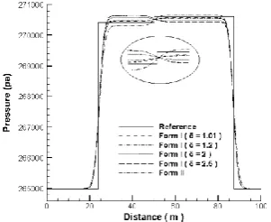
In order to predict pressure changes profile and more accurate matching of results by analytical solution Toumi’s shock tube case. The most appropriate amount of δ is 2; that ensures the roots of the characteristic equation are real, as a results, the model is well-posed. Data are presented in Figure 19.
TABLE 2. Initial conditions of Toumi’s shock tube case
Quantity Unit Left Right
Gas volume fraction - 0.25 0.1
Liquid velocity 𝑚 𝑠⁄ 0 0
Gas velocity 𝑚 𝑠⁄ 0 0
Pressure 𝑚𝑝𝑎 20 10
Gas density 𝑘𝑔 𝑚⁄ 3 200 100
liquid density 𝑘𝑔 𝑚⁄ 3 1000 1000
Figure 17.Toumi’s Case. velocity profile of the gas phase for
the roots of characteristic equation of form (II)
Figure 18.Toumi’s Case. velocity profile of the gas phase for
the roots of characteristic equation of form (I)
Figure 19. Toumi’s Case. Comparison of the roots of the
characteristic equation of forms (I) and (II) for the pressure change profile
Figure 20. Toumi’s Case. Comparison of the roots of the
characteristic equation of forms (I) and (II) for volume fraction profile of the gas-phase
Figure 21. Toumi’s Case. Comparison of the roots of the
characteristic equation of forms (I) and (II) for velocity profile of gas phase
Figure 22. Toumi’s Case. Comparison of the roots of the characteristic equation of forms (I) and (II) for velocity profile of liquid phase
This model does not predict the motion of wave and it presents non-physical results due to having ill-posed model.
The pressure changes due to height of the fluid is used for calculating the roots of the characteristic equation of form II. But because of at the initial moment, there is pressure gradient around both sides of the diaphragm Toumi’s shock tube case. As a result, the pressure changes due to height of the fluid is intangible and the balance between the mathematical nature of physics model is not formed and therefore, system is ill-posed.
Results for pressure changes profile, volume fraction profile of the liquid phase, velocity profile of gas phase and velocity profile of liquid phase presented in Figures 19, 20, 21and 22, respectively are valid.
6. CONCLUSION
Our investigations indicated that the roots of the characteristic equation of form I ensures the range of well-posing more than the roots of the characteristic equation of form II. Results of Toumi’s shock tube case showed that extreme velocity and pressure gradients effect directly on the roots of the characteristic equation of two-fluid model and leads to present non-physical results for the roots of the characteristic equation of form II. The two-fluid model I is included a coefficient that appropriate selection of its value ensures that the roots of the characteristic equation is hyperbolic, but the roots of the characteristic equation have not this property.
7. REFERENCES
1. Issa, R. and Kempf, M., "Simulation of slug flow in horizontal and nearly horizontal pipes with the two-fluid model",
International Journal of Multiphase Flow, Vol. 29, No. 1, (2003), 69-95.
2. Omgba-Essama, C., "Numerical modelling of transient gas-liquid flows (application to stratified & slug flow regimes)", (2004), Ph.D. Thesis, School of Engineering Applied Mathematics and Computing Group, Cranfield University, UK. 3. Ishii, M., "Thermo-fluid dynamic theory of two-phase flow,
eyrolles, Physics Bulletin, Paris, Vol. 26, No. 12, (1975)
Eyrolles.
4. Ishii, M. and Mishima, K., "Two-fluid model and hydrodynamic constitutive relations", Nuclear Engineering and Design, Vol. 82, No. 2, (1984), 107-126.
5. Spalding, D., "Numerical computation of multi-phase fluid flow and heat transfer", Recent Advances in Numerical Methods in Fluids, Vol. 1, (1980), 139-167.
6. Ansari, M. and Shokri, V., "New algorithm for the numerical simulation of two-phase stratified gas–liquid flow and its application for analyzing the kelvin–helmholtz instability criterion with respect to wavelength effect", Nuclear Engineering and Design, Vol. 237, No. 24, (2007), 2302-2310.
7. Toro, E.F., "Riemann solvers and numerical methods for fluid dynamics: A practical introduction, Springer Science & Business Media, (2013) 2nd Edition, Springer
8. Evje, S. and Flåtten, T., "Hybrid flux-splitting schemes for a common two-fluid model", Journal of Computational Physics, Vol. 192, No. 1, (2003), 175-210.
9. Munkejord, S.T., Evje, S. and FlÅtten, T., "A musta scheme for a nonconservative two-fluid model", SIAM Journal on Scientific Computing, Vol. 31, No. 4, (2009), 2587-2622. 10. Shekari, Y. and Hajidavalloo, E., "Application of osher and
price-c schemes to solve compressible isothermal two-fluid models of two-phase flow", Computers & Fluids, Vol. 86, (2013), 363-379.
11. Wang, Z., Gong, J. and Wu, C., "Numerical simulation of one-dimensional two-phase flow using a pressure-based algorithm",
Numerical Heat Transfer, Part A: Applications, Vol. 68, No. 4, (2015), 369-387.
12. Bonizzi, M. and Issa, R., "A model for simulating gas bubble entrainment in two-phase horizontal slug flow", International journal of multiphase flow, Vol. 29, No. 11, (2003), 1685-1717.
13. Bonizzi, M. and Issa, R., "On the simulation of three-phase slug flow in nearly horizontal pipes using the multi-fluid model",
International Journal of Multiphase Flow, Vol. 29, No. 11, (2003), 1719-1747.
14. Carneiro, J., Fonseca Jr, R., Ortega, A., Chucuya, R., Nieckele, A. and Azevedo, L., "Statistical characterization of two-phase slug flow in a horizontal pipe", Journal of the Brazilian Society of Mechanical Sciences and Engineering, Vol. 33, No. SPE1, (2011), 251-258.
15. Hanyang, G. and Liejin, G., "Stability of stratified flow and slugging in horizontal gas-liquid flow*", Progress in Natural Science, Vol. 15, No. 11, (2005), 1026-1034.
16. Figueiredo, A.B., Bueno, D.E., Baptista, R.M., Rachid, F.B. and Bodstein, G.C., "Accuracy study of the flux-corrected transport numerical method applied to transient two-phase flow simulations in gas pipelines", in 2012 9th International Pipeline Conference, American Society of Mechanical Engineers., (2012), 667-675.
18. Ransom, V.H. and Hicks, D.L., "Hyperbolic two-pressure models for two-phase flow", Journal of Computational Physics, Vol. 53, No. 1, (1984), 124-151.
19. Coquel, F., El Amine, K., Godlewski, E., Perthame, B. and Rascle, P., "A numerical method using upwind schemes for the resolution of two-phase flows", Journal of Computational Physics, Vol. 136, No. 2, (1997), 272-288.
20. Evje, S. and Flåtten, T., "Hybrid central-upwind schemes for numerical resolution of two-phase flows", ESAIM:
Mathematical Modelling and Numerical Analysis, Vol. 39, No. 2, (2005), 253-273.
21. Cortes, J., Debussche, A. and Toumi, I., "A density perturbation method to study the eigenstructure of two-phase flow equation systems", Journal of Computational Physics, Vol. 147, No. 2, (1998), 463-484.
22. Toumi, I., "An upwind numerical method for fluid two-phase flow models", Nuclear Science and Engineering, Vol. 123, No. 2, (1996), 147-168.
Comparison of the Hyperbolic Range of Two-fluid Models on Two-phase Gas-liquid
Flows
H. Zolfaghary Azizia, M. Naghashzadegana, V. Shokrib
aDepartment of Mechanical Engineering, University of Guilan, Rasht, Iran
b Department of Mechanical Engineering, Sari Branch, Islamic Azad University, Sari, Iran
P A P E R I N F O
Paper history: Received 28August 2017
Received in revised form 28September 2017 Accepted 29October 2017
Keywords: Two-Phase Flow Two-Fluid Model Numerical Simulation Hyperbolic Analysis
ديكچ ه
هسیاقم یارب یددع هعلاطم کی ،هلاقم نیا رد یاه نایرج رب مکاح تباث امد یلایس ود لدم تلاداعم یکیلوبرپیه هدودحم
.تسا هدش ماجنا هلول لخاد یزافود یددع یزاسلدم راتسیاپ کاش ریخست دتم زا هدافتسا اب
ماجنا .تسا هدش تلاداعم
سنارفید مرف رد .تسا هدش هئارا مرف ود رد راشف حیحصت مرت عون ساسا رب یلایس ود لدم لی
I
راشف حیحصت مرت زا
مرف رد و کیمانیدوردیه
II
.تسا هدش هدافتسا کیتاتساوردیه راشف حیحصت مرت زا هسیاقم یارب
یکیلوبرپیه هدودحم
هنومن هلئسم زا ،هدش هئارا مرف ود رد یلایس ود لدم تلاداعم تعرس کاش هلول هنومن هلئسمود و مئاق هسدنه رد بآ ریش
.تسا هدش هدافتسا یمات کاش هلول و گرزب یبسن مرف یلایسود لدم
I
هب تبسن یرت هدرتسگ یراتفر شوخ هدودحم یاراد
مرف یلایس ود لدم
II
.دشاب یم مرف یلایس ود لدم
I
بیرض نیا یارب بسانم ریداقم باختنا هک دشاب یم یبیرض یاراد
مرف هصخشم هلداعم یاه هشیر اما ،دشاب یم هصخشم هلداعم یاه هشیر ندوب کیلوبرپیه هدننک نیمضت
II
ار تیلباق نیا