Heuristic Process Model Simplification in Frequency Response Domain

HEURISTIC PROCESS MODEL SIMPLIFICATION IN

FREQUENCY RESPONSE DOMAIN

M. Shirvani

Department of Chemical Engineering, Iran University of Science and Technology Narmak, Tehran, Iran 16844, [email protected]

M. A. Doustary

Department of Electrical Engineering, Shahed University Taleghani St., Tehran, Iran 15986, [email protected]

M. Shahbaz

Cement Research Center, Iran University of Science and Technology Narmak, Tehran, Iran 16844, [email protected]

Z. Eksiri

Department of Chemical Engineering, Amirkabir University of Technology Hafez Avenue, Tehran, Iran, [email protected]

(Received: June 7, 2003 – Accepted in Revised Form: February 26,2004)

Abstract Frequency response diagrams of a system include detailed and recognizable information about the structural and parameter effects of the transfer function model of the system. The information are qualitatively and quantitatively obtainable from simultaneous consideration of amplitude ratio and phase information. In this paper, some rules and relationships are presented for making use of frequency response information in order to identify the structure of rational and irrational models in a heuristic manner. Estimation of the values of the parameters are also accomplished in a graphical trial and error procedure. As an example, the heuristic method was applied for identifying the simplified model of a rotary cement kiln from the frequency response information of the analytically derived model of the system. The analytical model of the kiln, used in this paper, was obtained elsewere in a detailed procedure with some assumptions and by using initial and boundary conditions. Results obtained from identification of the simplified model for rotary cement kiln not only reveal the application of the heuristic method for model identification, but also demonstrate the appearance of unstable poles and zeros in the model of the system.

Key Words Heuristic Identification, Model Structure, Irrational Transfer Function, Distributed Parameter, Rotary Cement Kiln, Limited-Delay-Resonance, Unlimited-Delay-Resonance

ﻩﺪﻴﻜﭼ

ﻩﺪﻴﻜﭼ

ﻩﺪﻴﻜﭼ

ﻩﺪﻴﻜﭼ

ﺕﺍﺮﺛﺍ ﻦﻴﻨﭽﻤﻫ ﻭ ﺭﺎﺘﺧﺎﺳ ﺯﺍ ﻲﺼﻴﺨﺸﺗ ﻞﺑﺎﻗ ﻭ ﻞﻣﺎﻛ ﺕﺎﻋﻼﻃﺍ ﻱﻭﺎﺣ ﺎﻬﻤﺘﺴﻴﺳ ﻲﺴﻧﺎﻛﺮﻓ ﺦﺳﺎﭘ

ﻲﻣ ﻢﺘﺴﻴﺳ ﻲﻠﻳﺪﺒﺗ ﻊﺑﺎﺗ ﻝﺪﻣ ﻱﺎﻫﺮﺘﻣﺍﺭﺎﭘ

ﺪﺷﺎﺑ

.

ﺩﻮﻤﻧ ﻱﻭﺭ ﺯﺍ ﺕﺎﻋﻼﻃﺍ ﻦﻳﺍ

ﻪﭼ ﺯﺎﻓ ﻭ ﺎﻫ ﻪﻨﻣﺍﺩ ﺖﺒﺴﻧ ﻱﺎﻫﺭﺍ

ﺖﺳﺍﺱﺮﺘﺳﺩﺭﺩﻲﻤﻛ ﺕﺭﻮﺼﺑﻪﭼ ﻭﻲﻔﻴﻛﺕﺭﻮﺼﺑ

. ﺕﺎﻋﻼﻃﺍﺯﺍﻩﺩﺎﻔﺘﺳﺍﻱﺍﺮﺑﻲﻄﺑﺍﻭﺭﻭﺪﻋﺍﻮﻗﻪﻟﺎﻘﻣﻦﻳﺍﺭﺩ

ﻲﻧﺩﺮﺑﻲﭘ ﺕﺭﻮﺼﺑ ﺎﻬﻧﺁ ﻲﻳﺎﺳﺎﻨﺷﻭﺎﻳﻮﮔ ﺮﻴﻏﻭ ﺎﻳﻮﮔﻱﺎﻫ ﻢﺘﺴﻴﺳ ﻝﺪﻣﺭﺎﺘﺧﺎﺳ ﺺﻴﺨﺸﺗ ﻱﺍﺮﺑﻲﺴﻧﺎﻛﺮﻓﺦﺳﺎﭘ

ﺖﺳﺍﻩﺪﺷﻪﺋﺍﺭﺍ

.

ﻧﻝﺪﻣﻱﺎﻫﺮﺘﻣﺍﺭﺎﭘﺮﻳﺩﺎﻘﻣﻦﻴﻤﺨﺗ

ﺖﺳﺍﻩﺪﺷﻡﺎﺠﻧﺍﻲﻜﻴﻓﺍﺮﮔﻱﺎﻄﺧﻭﺱﺪﺣﺕﺭﻮﺼﺑ ﺰﻴ

.

ﻥﺍﻮﻨﻌﺑ

ﻥﺎﻤﻴﺳﺭﺍﻭﺩ ﻩﺭﻮﻛﻚﻳﻲﺴﻧﺎﻛﺮﻓﺦﺳﺎﭘﺕﺎﻋﻼﻃﺍﺯﺍ،ﻪﻟﺎﻘﻣﺭﺩﻩﺪﺷ ﻪﺋﺍﺭﺍﻲﻧﺩﺮﺑ ﻲﭘﺵﻭﺭﻥﺩﺍﺩ ﻥﺎﺸﻧﻱﺍﺮﺑ ،ﻝﺎﺜﻣ

ﺖﺳﺍ ﻩﺪﺷﻩﺩﺎﻔﺘﺳﺍ،ﻢﺘﺴﻴﺳﻱﺍﺮﺑﻩﺪﻣﺁﺖﺳﺪﺑﻲﻠﻴﻠﺤﺗﻝﺪﻣﻪﺑ ﻁﻮﺑﺮﻣ

. ﻱﺎﺟﺭﺩﻪﻟﺎﻘﻣ ﺭﺩﻪﺘﻓﺭ ﺭﺎﻜﺑﻲﻠﻴﻠﺤﺗﻝﺪﻣ

ﻔﻣﺭﻮﻄﺑﻱﺮﮕﻳﺩ

ﺖﺳﺍﻩﺪﻣﺁﺖﺳﺪﺑﻱﺯﺮﻣﻂﻳﺍﺮﺷﻦﻴﻨﭽﻤﻫﻭﻪﻴﻟﻭﺍﻂﻳﺍﺮﺷﻭﺎﻬﺿﺮﻓﻲﻀﻌﺑﺯﺍﻩﺩﺎﻔﺘﺳﺍﺎﺑﻞﺼ

.

ﺞﻳﺎﺘﻧ

ﻲﻣﻥﺎﻴﺑﺍﺭﻪﻟﺎﻘﻣﻦﻳﺍﺭﺩﻩﺪﺷﻪﺋﺍﺭﺍﻲﻧﺩﺮﺑﻲﭘﺵﻭﺭﺩﺮﺑﺭﺎﻛﻪﻜﻨﻳﺍﻦﻤﺿ،ﻩﺪﺷﻩﺩﺎﺳﻝﺪﻣﻲﻳﺎﺳﺎﻨﺷﺯﺍﻞﺻﺎﺣ

،ﺩﺭﺍﺩ

ﺮﺨﻣﻭﺕﺭﻮﺻﺭﺍﺪﻳﺎﭘﺎﻧﻱﺎﻫﻪﺸﻳﺭﻥﺎﻤﻴﺳﺭﺍﻭﺩﻩﺭﻮﻛﻝﺪﻣﺭﺩﻪﻛﺖﺳﺍﺐﻠﻄﻣﻦﻳﺍﻱﺎﻳﻮﮔ

ﺩﺭﺍﺩﺩﻮﺟﻭﺝ

.

1. INTRODUCTION

Frequency response diagrams include detailed and

frequency response data helps in a delicate manner in identifying the structural aspects of the model of a system. The information can very well be detected from both qualitative and quantitative points of view from the amplitude ratio and phase diagrams of the system. From the apparent behavior of the diagrams, one can recognize the lumped or distributed parameter nature as well as other structural aspects of the model of the system. The essential recognizable information are the difference between the orders of denominator and numerator of the transfer function, as well as the appearance of origin located poles or zeros, and the appearance of minimum or non-minimum phase behavior of the model. Also, the existence of unstable poles or zeros in the model are well recognizable from the intermediate and high frequency information. On the other hand, the appearance of periodic resonance in both amplitude ratio and phase diagram is an indication of irrational form of the structure of the model of the system. The values of the model parameters can still be determined in a heuristic manner. The procedure of heuristic identification of model structure and parameter estimation, presented in this paper, finds its important applications very well in process systems which mostly are inherently distributed parameter in their nature and thus the problem of choosing a model structure for the system becomes more complicated than the lumped parameter systems. Such kinds of process systems consist of packed column and rotary drum systems, as well as shell and tube heat exchangers, which include the common physical nature of two flowing streams in parallel or counter flow.

In this paper, frequency response information of an analytically derived complex model of a rotary cement kiln is used for identifying the structure as well as the parameters of the simplified model of the system in a heuristic manner. The rotary cement kiln is a distributed parameter process system with the longitudinal dependence of the variables being more important than their radial or angular dependencies. Thus, it seems that an irrational simplified transfer function model structure consisting of parallel combination of two rational transfer functions is quite capable in describing and fitting the dynamic behavior of the system. Actually, it is very difficult to apply the conventional identification techniques for this system [1]. Whereas the heuristic technique applied here can

be used to identify the structure of the model of the system.

2. ANALYTICAL MODEL OF ROTARY CEMENT KILN

Like many other process systems, the rotary cement kiln is a distributed parameter process system in which the transportation of materials (including solid and gas) is the dominant phenomena in the system. However, many other important phenomena occur in the system. These include: intensive radiation of flame (especially in the burning zone), formation and variation of the thickness of the coating layer in the burning zone, and the calcination of the calcium carbonate and transportation of CO ₂ gases from flowing solid to the gas stream (appearing only in the calcining zone of the kiln). Since the procedures of derivation of the analytical model are very complicated, here only a brief explanation of the assumptions, as well as the procedures of developing the model is presented. Such distributed parameter systems are referred to as quasi-rational distributed systems (QRDS) [2,3] and their simplified transfer functions are constructed from parallel combination of two rational transfer functions, which at least one of them include time-delay parameter. This time-time-delay parameter, in contrast to the time-delay parameter of rational models, depending on the values of the other parameters in the model, may show complete characteristics of a time-delay (TD) parameter or a quasi-time-delay (QTD) characteristic. We refer to the (QTD) characteristic as the situation in which a limited effect on phase diagram at high frequencies appears, despite the existence of time delay parameter in the model. Quasi-rational distributed systems exhibit a periodic resonating behavior in frequency response diagrams both in amplitude ratio and phase.

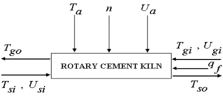
for the sake of better understanding the subject, a brief explanation of the model derivation is also discussed here. The details of the complicated analytical model, including procedures of derivation are given elsewhere [4]. It is necessary to note that we do not claim anything about applicability of the model presented here, since there have been some big assumptions applied during model derivation. The analytical model of the system is derived by use of some assumptions and application of heat balance on the essential individual elements of the system, including the kiln shell as well as the gas and solid materials [5]. The resulting nonlinear partial differential equations from the energy balances were combined with the model of transportation of solid materials in rotary drums [6]. This was done for the purpose of inserting the variable “n” (the drum’s rotation speed) in the model. This variable is an important controlling variable for such systems. The outside temperature and the wind velocity were also included in the model by considering the heat transfer between the shell and the flowing ambient air (wind) outside the kiln. At the same time, the parameters of time and length in the model were changed to their dimensionless forms by dividing them by the residence time of solid material inside the kiln and the length of kiln, respectively. Then, the model was linearized around the operating point and the resulting linearized model, which included eight input and two output variables were solved analytically by considering the boundary conditions to obtain sixteen various transfer functions of the system. The input and output variables considered in the model are shown in Figure 1.

The velocity of solid material and flowing gas were assumed to be independent of distance in the kiln. These additional assumptions were required to be included for reducing the number of unknowns. In this way the model becomes exactly specified with degree of freedom equal to zero. Due to these additional assumptions, some expected changes in the results of simulating the model were observed, which are discussed later during model simplification studies. The resulting model of the system was very complicated with a great number of replacing variables and parameters. This was due to the linearizations, which was performed on the individual terms of the model, and also due to the analytical procedure that was applied for solving the set of equations [4]. In fact, the resulting complicated model, although very detailed in its nature, could not explicitly express anything regarding the dynamics of system unless it is simplified in the form of standard models for dynamic systems; like transfer functions. It should be considered that the model, due to its analytical nature, depending on various assumptions applied in its derivation, is quite able to reflect the inherent dynamical aspects of the system. Thus, the conclusions of the paper is twofold, in that it reflects not only some specific dynamic characteristics of rotary cement kilns, but also presents a new heuristic method in frequency response domain for determining the structure of the simplified model of a system and identifying the values of its parameters.

3. SIMULATION AND QUALITATIVE MODEL VALIDITY

The resulting analytical model is simulated in frequency domain for individual transfer functions. The simulation is performed by use of MATLAB software. The results of simulation can be used not only for identifying the simplified transfer functions of the system, but also to investigate the model validity in a qualitative manner. The results of simulation both for the analytically derived model and the heuristic derived and simplified one are shown in comparison in Figures 2 through 17 for various transfer functions.

Although the heuristic identification of simplified

Figure 2. Frequency response simulation for GTsi,Tso(s).

Figure 4.Frequency response simulation for GUsi,Tso(s).

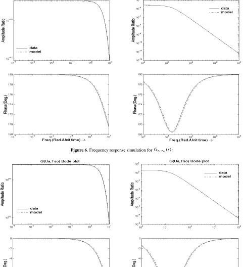
Figure 6.Frequency response simulation for GTa,Tso(s).

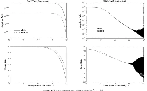
Figure 8.Frequency response simulation for G_qf,Tso(s).

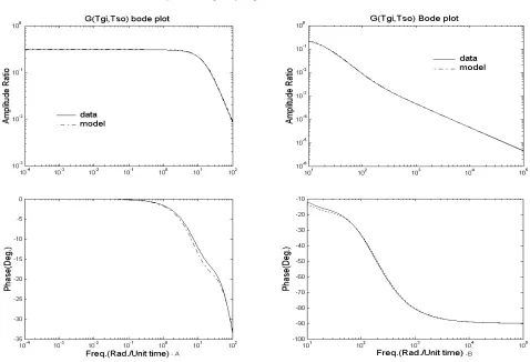
Figure 10.Frequency response simulation for GTsi,Tgo(s).

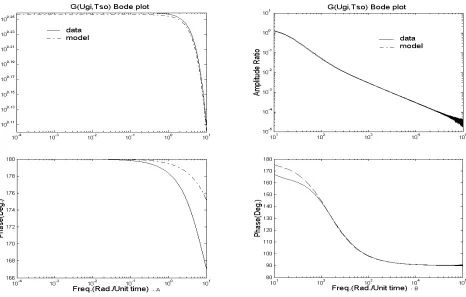
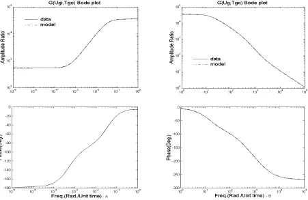
Figure 12.Frequency response simulation for GUsi,Tgo(s).

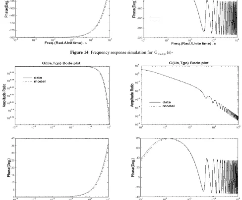
Figure 14.Frequency response simulation for G_Ta,Tgo(s).

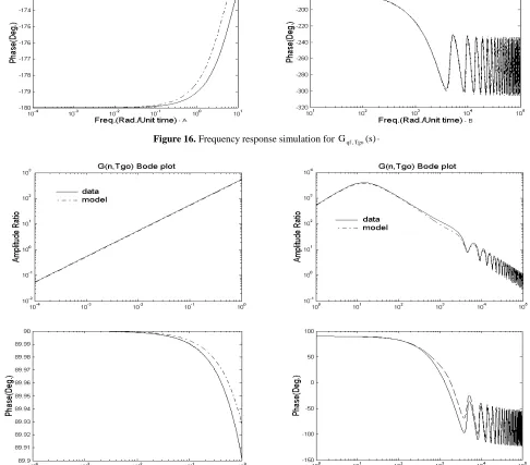
Figure 16. Frequency response simulation for G_qf,Tgo(s).

model is discussed later, in order to avoid repetition of graphs, the simulation of simplified model is also represented simultaneously in Figures 2 to 17. Each of the Figures is divided into two parts, one for lower frequencies and the other for higher frequencies. This is done since we are interested in having a clear observation of the system behavior from sufficient low frequencies up to sufficient high frequencies to help for better recognition of the effects of existing dynamical elements of the system. In these Figures

ω

is in Rad./(Unit Time), where the unit of time is the retention time of solid material while passing through the drum, in the vicinity of operating conditions.

Before getting into the details of the procedures for heuristic identification of the simplified model, it is well suited here to have a discussion about the validity of the complex analytical model. From qualitative validity point of view, the following points can be discussed:

1. In the diagrams relating to the input n, the rotational speed of the kiln (Figures 9 and 17), contrary to all the other inputs, low frequency slopes equal to +1are visible in amplitude ratio diagrams. This means that the transfer functions for this input should be differentiating ones (with a zero in the origin). In other words, the

step response curve will have a new steady state value equal to its initial steady state value prior to insertion of the input. This conclusion is well in accordance with physical implication of the system. Since it is recognizable that, for a change in the speed of rotation of the drum, there will not be any sustained change in the output temperatures, if no additional input or output energy is affecting the system.

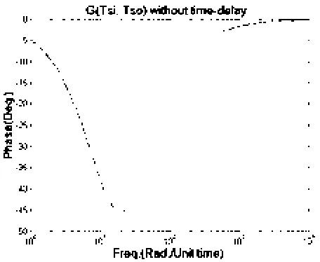
2. It is expected that the diagrams of phase show a limit value at high frequencies, for cases in which the inputs and outputs are located in one end of the kiln. Contrary to this, for cases in which the related inputs and outputs are located in opposite ends, the phase diagrams should exhibit the existence of the effects of time-delay parameters. This means no approach to any limiting value at high frequencies in phase diagrams. Thus according to Figure 1, we expect to observe the phase part of the diagrams relating to G_Tsi,Tso(s) (Figure 2), G_Usi,Tso(s)

(Figure 4), G_Tgi,Tgo(s) (Figure 11), G_Ugi,Tgo(s)

(Figure 13) and G_qf,Tgo(s)(Figure 16) exhibit no limited values at high frequencies, due to the effect of the respective delay times. However, this behavior can only be observed in Figures 2 and 11 for G_Tsi,Tso(s) and G_Tgi,Tgo(s), while for the other three (Figures 4, 13 and 16), the phase diagrams do not show any such effect. This problem is a straight result of the exerted assumptions during the procedures of deriving the analytical model. Firstly, the assumption of independence of velocities of gas and solid phase on the distance in the drum has resulted in disappearance of the effects of time-delay parameters in the velocity input diagrams (Figures 4 and 13). Secondly, concerning the input q_f (the heat of combustion), its related term in the model is inserted in equations without any differentiation with respect to time or any dependence to the velocity of flowing gas. Thus, the effect of time-delay could not be traced in its phase diagram in Figure 16. In fact, it is a reasonable assumption that the time-delay for gas velocity and heat of combustion inputs are the same as the time-delay for gas temperature input affecting the temperature of gas at the output. In the same manner, we may

Figure 18. Phase diagram of GTsi,Tso(s) after elimination of

assume that the time-delay for solid velocity input is the same as the time-delay for solid temperature input affecting the solid temperature output at the other end of the kiln. In this way, the missing time-delay effects in the Figures 4, 13 and 16, can be recovered in the procedures of identifying the simplified model from the frequency response of the complex analytical model. This is the task, which is done later in deriving the simplified model for system.

3. Some of the Figures exhibit periodic resonance behavior, with the same periods of oscillation coexisting in both the amplitude ratio and phase diagram. Such behavior in frequency response, which we expect to be a specific characteristic of distributed parameter process systems with two flowing streams, is frequently reported for shell and tube heat exchangers from long time ago [7,8]. For this type of heat exchangers it is known that the transfer function model of the system is in the form of irrational transfer function, which is the combination of two transfer functions in parallel, one of which includes time-delay parameter. Furthermore, it is known that for such models there will appear periodic resonance in frequency response.

4. HEURISTIC IDENTIFICATION OF SIMPLIFIED MODEL

In developing the heuristic identification of the simplified model from the frequency response data, we make a distinction between the rational and irrational transfer function models. The structure of irrational model considered here, is very well suited for describing the class of distributed parameter process systems in which the axial transportation of materials is the dominant phenomenon affecting the dynamic characteristics of the system. For such systems, the simplified models can be considered in the form of parallel combination of two rational transfer functions which at least one of them will include time-delay parameter. As an example, among the sixteen transfer functions discussed in this paper for the rotary cement kiln, five of them are explicitly observed to have periodic resonance characteristics. Therefore,

the irrational transfer functions are well suited for demonstrating their specific dynamic behavior. In fact, many of the diagrams represented in Figures 2 to 17, include some irregular resonance, which can be observed at high frequencies. These are appearing after the regular resonance. The irregular resonance were neglected here to be modeled, because it would be a very difficult task and requires much prior knowledge of the dynamics of more complicated irrational models to enable one to detect and identify the structure of such characteristics. Therefore, this part of diagrams are omitted from the Figures 2 to 17, except the two Figures 5 and 8 (relating to GUgi,Tso(s)and

) s (

G_qf,Tso ), which are shown only for demonstrating this type of behavior. Concerning to Figure 8, attempts were made to demonstrate the irregular resonance by using some additional terms in the simplified model. But, as seen in this Figure the results of fitting are not so much excellent although that it is not up to very high frequencies. The details of the irregularities of the model are reflected in [4].

4a. Identification of Rational Transfer

Function Models

For the case under study, the system can be considered as a non-resonating one demonstrated by the following transfer function model:

s d

e ) 1 s (

) 1 s ( s K ) s (

G _n

1 i

i , D m

1 j

j , N p

r

τ

−

= =

∏

∏

+ τ

+ τ

= (1)

In this model, the parameter

n

;

n

=

1

,

2

,

3

,

L

is the number of poles of denominator that are not located in the origin (non-integrating poles). Also,

L

, 3 , 2 , 1 , 0 m ;

m = is the number of zeros of

numerator that are not located in the origin (non-differentiating zeros) and p; p=L,−2,−1,0,1,2,L

is the number of poles or zeros that are located in the origin (differentiating poles or integrating zeros). Thus, the order of numerator and denominator are

, p m

, m

D_N = p≤0

, n

DD = p≥0

, p n

DD = − p<0

The overall order of the model is m+p−n. The parameters

τ

D,i and

τ

N,j represent the time constants, Kis the steady state gain of the model, and

τ

_d

;

τ

_d

≥

0

, is the time-delay parameter of the model. Here, in the example of rotary cement kiln, we are not faced with the cases were the complex roots should be considered in the model. Nevertheless, for such cases of non-periodic resonance systems determination of damping parameter as well as the time constant from the frequency response data are also possible [9]. Each of the time constants “

τ

” are related to its affecting frequency, by:

τ

ω = τ

c

1

(2)

where,

ω

_cτ is the corner frequency at which the parameter

τ

affects the amplitude ratio and phase. Therefore, it is possible to predict the approximate values of time constant parameters by considering the changes in the slope of amplitude ratio curve as well as the changes in the phase diagram in the vicinity of each visible

ω

_cτ.

The order of repetition of an especial time constant parameter can be detected from the order of changes in the slope of amplitude ratio. The change in the slope of amplitude ratio should be

1

+ for each of the appearing zeros in the model and it is 1− for each of the poles. Thus, all of the poles and zeros appearing in the model affect the overall slope of amplitude ratio at high frequency. It is notable that, there is no effect from the sign of the poles or zeros (stable or unstable poles or zeros) on the slope changes appearing in amplitude ratio.

There would be corresponding changes in the phase. Contrary to the changes which appear in the slope of the amplitude ratio, in the case of phase the changes are dependent on the fact that the pole

or zero is located in the RHP or in the LHP of the complex coordinate. In total, there appear four different cases regarding the stable and unstable poles and zeros in the frequency response diagrams. These are as follows:

1. For each of the stable zeros, there appears a

90

+ degrees change in ultimate value of phase diagram at high frequencies, and an increase equal to one in the slope of amplitude ratio.

2. For each of the unstable zeros, there appears a

90

− degrees change in ultimate value of phase diagram at high frequencies, and an increase equal to one in the slope of amplitude ratio.

3. For each of the stable poles, there appears a

90

− degrees change in ultimate value of phase diagram at high frequencies, and a decrease equal to one in the slope of amplitude ratio.

4. For each of the unstable poles, there appears a 90

+ degrees change in ultimate value of phase diagram at high frequencies, and a decrease equal to one in the slope of amplitude ratio. These concepts, not only help in recognizing the values of time constant parameters very well, but also their stable or unstable characteristics can be checked and determined directly. After determination of the approximate values of time constants and their respective stability, their improved values can be obtained graphically in a trial and error effort by comparing the model and data.

In order to identify the structure of the model, it is needed to determine the orders of numerator and denominator, as well as the number of each of the stable and unstable poles and zeros. Also, it is necessary to determine the sign of the steady state gain of the model. These are the prerequisites, before starting to determine the values of parameters which can be done graphically in a trial and error procedure. In order to accomplish the above task, the following rules can be used straightly for identification of rational models from frequency response data. These rules are relevant to low and high frequencies as well as the intermediate frequency information.

T hat is, if the dynami c element sp; ... , 2 , 1 , 0 , 1 , 2 ...,

p= − − is affecting the behavior of the model, then, the low frequency asymptote with slope equal to p will occur in amplitude ratio. Also the phase diagram of the model will show a jump equal to 90 at all frequencies. Therefore, if p

0

p> , the jump will be in upward direction, and if

0

p< , it will be in downward direction. Since this jump appears at all frequencies, therefore its effect can be detected at high frequencies as well as low frequencies. In the example of rotary cement kiln, for the graphs relating to speed of rotation of drum, low frequency slope of amplitude ratio is recognized to be equal to

+

1

, while for all the other inputs it is equal to zero.

A2. High frequency slope of the asymptote of amplitude ratio diagram is an indication of the difference between the orders of the polynomials of numerator and denominator (D_M =D_N −D_D; D_M =0,−1,−2,...).

If the resonating characteristics appear in the frequency response diagrams, it is possible to consider two upper and lower envelops both for amplitude ratio and phase diagrams. In the example of rotary cement kiln, the upper and lower envelops for amplitude ratios appear to be parallel at high frequencies (at least up to frequencies under our consideration). Therefore, the slope of amplitude ratio at high frequency can be considered as the slope of one of these envelops.

A3. In addition to the above jumps and ultimate effects on the phase diagram, there will be other all-frequency phase jump effects which results from the existence of negative sign in the steady state gain of the system. Therefore, if K<0, then without any effect on amplitude ratio the phase diagram will jump an amount equal to

180

+ degrees towards the upward direction or

180

− degrees towards the downward direction. The direction of jump depends on weather the phase diagram exhibits a positive slope or a negative slope at low frequencies (see the Figures 12, 14, 15, 16 and 17).

A4. It is worth noting that the slope of asymptote of amplitude ratio at high frequencies is independent of the sign of the time constants in the

numerator or denominator (LHP or RHP roots). These effects of high frequencies for amplitude ratio are similar to the intermediate effects stated before.

The following equations can describe the relation between high frequency asymptote of amplitude ratio as well as the high frequency phase values with the LHP and RHP poles and zeros of the model. p ) D D ( ) D D ( D D

S_H = _N − _D = _NL + _NR − _DL + _DR +

(3)

[

]

0 K , 180 ) D D ( 90 S 90 p ) D D ( ) D D ( P DR NR H DR DL NR NL H > − − ⋅ = + − − − = (4) 0 K , 180 P

PH,K = H ± < (5)

From the above equations it is not possible to determine in an explicit manner the four unknowns

NL

D , D_NR, D_DL and D_DR with prior information of p , SH and P or H PH,K. Thus, heuristic determination of the above unknowns finds its application for identifying a full precise model from the data.

A5. In both amplitude ratio and phase, the neighboring stable poles and zeros or neighboring unstable poles and zeros will cancel the effects of each other at high frequencies. These roots can be detected from trends of increases or decreases in the diagrams at intermediate frequencies. If these kinds of poles and zeros are neglected, then, around their affecting frequency, there will appear some deviations in fitness of model and data. A6. If the data show the effects of time delay parameter (specially large amount of parameter) then this parameter should be determined at first. This can be done in a graphically trial and error procedure, such that the ultimate value of phase becomes recognizable. In this way, the details of the effects of time constant parameters as well as the steady state gain on phase become apparent. This is the effort, which has been made exactly for

) s (

parameter is large enough to diminish the effects of other time constant parameters. In Figure 18 the same phase diagram of Figure 2 – B is shown after elimination of time-delay effect.

4b. Identification of Irrational Transfer

Function Models

An irrational transfer function model of the structure shown in 6 is well suitable for identifying the frequency response data of Figures 12, 14, 15, 16, and 17, relating to G_Usi,Tgo(s),

) s (

G_Ta,Tgo , G_Ua,Tgo(s), G_qf,Tgo(s) and G_n,tgo(s), respectively. These Figures demonstrate periodic

resonance both in their amplitude ratio and phase.

s s

td d

2 n

1 k

k , 2 D 2 m

1 l

l , 2 N p 2

1 n

1 i

i , 1 D 1 m

1 j

j , 1 N p 1

ir

e e ) 1 s (

) 1 s ( s K

) 1 s (

) 1 s ( s K

) s ( G

τ − −

= = =

=

   

 

+ τ

+ τ 

  

 

+ + τ

+ τ =

∏

∏

∏

∏

(6)

Figure 19. Frequency response of the distributed model representing limited-delay-resonating phase characteristics

1 s e 1 s

2 . 1 ) s ( G

s 25 . 0

+ + +

= − . Figure 20_{representing unlimited-delay-resonating phase characteristics}. Frequency response of the distributed model

1 s

e 2 . 1 1 s

1 ) s ( G

s 25 . 0

+ + +

Here also, a structure with no complex roots in the simplified model is considered, since an under damped behavior is not observed in the Figures. An example of finding a simplified process model for such a distributed parameter system, which includes complex poles, is available elsewhere [10].

In this model the explicit time-delay parameter is

τ

_d, while the parameter

t

_d can be considered as a quasi-time-delay parameter since it may represent either an unlimited-delay effect or a limited-delay effect in the phase diagram. The difference between the two cases of limited-delay effect and unlimited-delay effect is shown in Figures 19, 20 and 21. As is shown in these Figures, the phase diagram may change significantly with a slight change in the amount of the parameters K₁ and

2

K [11,12].

In the frequency response diagrams for rotary cement kiln, no such examples of unlimited-delay phase characteristic are observed. However, such transcendental dynamic characteristics have been observed for similar distributed parameter process systems [8]. The rules that can be stated for heuristic identification of the elements in the structure of the model of such systems are discussed bellow. Actually, these rules should be used in connection to the previously stated rules for rational models.

B1. As in model 1, the parameter p can be determined from the slope of the asymptote of amplitude ratio at low frequencies. This is a case, appearing in Figure 17 for input n and output T . It should be noted that the term _g “sP” should appear similarly in both parts of the simplified model of rotary cement kiln. Also, in the same way as the rational models, the term “sp” causes the phase diagram to have a jump equal to 90 at all p frequencies.

B2. At high frequencies, the upper and lower envelopes of resonating amplitude ratio diagram are parallel lines with some specific slopes, which means that the slope of individual rational parts of the model are equal at high frequencies (

S

H1

=

D

N1

−

D

D1

=

S

H2

=

D

N2

−

D

D2)

[11].

B3. In model 6 the period of resonance at low and middle frequencies depends on time constant parameters as well as the parameter

t

d. At sufficiently high frequencies, where the effect of time constant parameters can almost be

Figure 21. Effect of time-delay parameter on the frequency response behavior of distributed model, representing limited-delay-resonating phase characteristics

s s

e s e s s

G 0.25

25 . 0

1 1

2 . 1 )

( −

−

   

 

+ + +

neglected, the parameter

t

_d will become the main affecting parameter on period of resonance [11]. Thus, it is possible to determine the value of

t

_d in a graphical trial and error procedure by adjusting the period of model to the period of data at middle and high frequencies.

B4. At low frequencies the periods of resonance are affected by all the parameters except

τ

d,

1

K

and

K

2. However, the algebraic signs for 1

K

and K2 straightly affect the first period of resonance as well as the

±

180

deg

rees

jumps in phase. The appearance of a half or a complete resonance in the first period, may be checked by comparing with the next coming period(s) in the graph. The above statements are summarized in Table 1, which can help very well to recognize the respective signs and relative values of the parameters K1 and K2 from the apparent behavior of amplitude

ratio and phase at low frequencies. The final values of these parameters can then be obtained by trial and error in a graphical mode.

B5. The width of periodic resonance, or in other words, the vertical distance between the upper and lower envelopes at high frequencies is a function of

K

′

=

K

₁

−

K

₂ . As the value of

K

′

decreases the distance between the upper and lower envelopes increases, such that at

0

K′= , the distance reaches to its maximum value, both in amplitude ratio and phase. For phase diagram the maximum width, corresponding to K′=0, is equal to 180

degree [11,12]. Using this fact and also noting that the absolute value of overall gain of the model

K

_1,2

=

K

₁

+

K

₂ can be determined directly from the low frequency value of amplitude ratio, and also considering the notation B2, the signs and the values of the

TABLE 1. Determination of Parameters K1 and K2 from Low Frequency Information.

Relative conditions

of steady-state gains

Condition of first period of resonance in amplitude

ratio

Appearance of jump effect in phase equal to ±180degrees

1

K

₁

f

0

K

₂

f

0

,

K

₁

f

K

₂ half period no

2

K

1

f

0

K

2

f

0

,

K

1

p

K

2 half period no

3

K

₁

f

0

K

₂

p

0

,

K

₁

f

K

₂ complete period no

4

K

₁

f

0

K

₂

p

0

,

K

₁

p

K

₂ complete period yes

5

K

₁

p

0

K

₂

f

0

,

K

₁

f

K

₂ complete period yes

6

K

1

p

0

K

2

f

0

,

K

1

p

K

2 complete period no

7

K

₁

p

0

K

₂

p

0

,

K

₁

f

K

₂ half period yes

parameters K1 and K2 can be determined graphically in a trial and error procedure.

B6. For the case of Figures 9 and 17, in which the slope of amplitude ratio at low frequency is not zero, determination of the values of gains “

K

” in model 1, and “K1,2 = K1 + K2” in model 6 can be done from the values of amplitude ratios at ω=1. By use of the above rules, all of the five diagrams, which possess resonating characteristics, are fitted heuristically with the simplified models of irrational structure.

B7. In the case of rotary cement kiln, in all of the five diagrams which demonstrate periodic resonance characteristics, the phase diagrams are approaching to some limiting range at high frequencies without demonstrating the infinite phase characteristics of a time-delay parameter (similar to Figure 20). This means that

K

1

f

K

2 [11,12]. Thus, the rotary cement kiln model is related only to the rows 1, 3, 5 and 7 in Table 1. Now, by use of the above information, and noting the appearance of a complete or half period resonance in amplitude ratio as well as the appearance of ±180degrees jump in phase diagrams, it would be possible to determine the related row in Table 1, from which the signs of parameters

K

₁ and

K

₂are determined. In this manner, after determining the signs of the parameters

K

₁ and

K

₂, their precise values can be determined in a graphical trial and error effort such that

K

₁

>

K

₂ and the low frequency gains of model and data become exactly fitted.

B8. In the case of rotary cement kiln model, the effects of parameter

τ

dcannot be detected in any one of the diagrams. Thus, in any of the five resonating cases it is concluded that

0

d

=

τ

, while the parameter

t

d

≠

0

since there are periodic resonance in the diagrams. After determination of parameters

p

and

τ

d, the time constant parameters “

τ

” as well as the quasi-time-delay parameter “

t

d” can be determined by considering the rules B2 and

B3 in a graphical trial and error procedure. If the parameter

τ

_dexists in the model, it should be determined prior to time constants in a graphical trial and error sense, because the effects of this parameter prevents from clear observation of the effect of time constants. The results of application of the above rules and statements to the cement kiln are the following simplified transfer functions. It is seen that the system is an unstable distributed parameter one: s e s s s

G_{TsiTso 2 2} 1.01

2 2 6 , ) 1 10 45 . 3 ( ) 1 10 8 . 7 ( 10 03 . 1 ) ( − + × − + × − × = − ₋ − (7) ) 1 s 10 0 . 5 ( ) 1 s 10 5 . 7 ( ) 1 s 10 6 . 5 ( 10 1 . 3 ) s (

G _{2 2}

3 1 Tso , Tgi + × − + × + × − × = ₋ − − ₋ (8) s 01 . 1 e ) 1 s 10 55 . 7 ( ) 1 s 10 5 . 28 ( 10 54 . 1 ) s ( G ₂ 1 2 Tso , Usi − + × + × × = ₋ − (9) ) 1 s 10 75 . 6 ( ) 1 s 10 75 . 6 ( ) 1 s 10 0 . 7 ( 805 . 1 ) s (

G _{2 2}

) 1 s 10 34 . 7 ( s 8 . 2095 ) s (

G_{n,Tso 2}

+ ×

−

= ₋ (14)

) 1 s 10 1 . 5 ( ) 1 s 10 3 . 7 ( ) 1 s 10 0 . 7 ( 10 02 . 2 ) s (

G _{2 2}

4 2 Tgo , Tsi + × − + × + × − × − = ₋ − −₋ (15) s 00033 . 0 e ) 1 s 10 06 . 3 ( ) 1 s 10 83 . 2 ( ) s (

G _{2 2}

2 2 Tgo , Tgi − + × − + × −

= ₋− (16)

) 1 s 10 95 . 6 ( ) 1 s 10 95 . 6 ( ) 1 s 10 75 . 7 ( ) 1 s 10 75 . 4 ( ) 1 s 10 25 . 4 ( 48 . 2 ) s ( G 2 2 4 4 2 Tgo , Usi + × − + × + × + × − + × − × = − − − − s 00138 . 0 e ) 1 s 10 0 . 7 ( ) 1 s 10 0 . 5 ( ) 1 s 10 25 . 4 ( 10 68 . 0 4 4 2 4 − + × + × + × − × −

+ ₋ − ₋ (17)

) 1 s 10 06 . 7 ( ) 1 s 8 . 28 ( ) 1 s 10 92 . 1 ( 10 37 . 5 ) s ( G 2 3 2 Tgo , Ugi + × + − + × × − = ₋ s 00033 . 0 e ) 1 s 10 526 . 2 ( 1 s 10 645 . 5 3 4 − − − + × + × − × (18) ) 1 s 10 5 . 2 ( ) 1 s 10 6 . 6 ( 10 36 . 1 ) s (

G _{2 3}

5 Tgo , Ta + × + × − × − = ₋ − ₋ s 00138 . 0 e ) 1 s 10 5 . 2 ( ) 1 s 10 6 . 6 ( 10 7 . 7 3 2 6 − − − − + × + × − × + (19) ) 1 s 10 5 . 2 ( ) 1 s 10 6 . 6 ( 57 . 10 ) s (

GUa,Tgo _{2 3}

+ × + × − = _{− −} s 00138 . 0 e ) 1 s 10 5 . 2 ( ) 1 s 10 6 . 6 ( 0 . 6 3 2 − − − _{+ × +} × − − + (20) s 00033 . 0 s 00137 . 0 e e ) 1 s 10 51 . 2 ( 10 11 . 5 ) 1 s 10 51 . 2 ( ) 1 s 10 1 . 1 ( ) 1 s 10 62 . 9 ( 10 0 . 1 ) s ( G 3 6 3 1 2 5 Tgo , qf − − − − − − − −             + × × + + × + × − + × − × − = (21) ) 1 s 10 95 . 6 ( ) 1 s 10 95 . 6 ( ) 1 s 10 75 . 7 ( s ) 1 s 10 75 . 4 ( 10 24 . 5 ) s ( G 2 2 4 4 2 Tgo , n + × − + × + × + × − × = − − − − s 00138 . 0 e ) 1 s 10 8 . 7 ( ) 1 s 10 8 . 5 ( s 10 7 . 1 4 4 2 − + × + × × − + ₋ − ₋ (22) 5. CONCLUSION

Frequency response diagrams include complete information about the details of structure and individual elements of the model of the system. These information can be detected heuristically by use of some rules and relationships which are presented for identifying the structure of the model of the system. The rules were presented for rational as well as irrational transfer function models. Primary estimations of the amounts of the parameters of the model are possible by considering the region of frequencies in which some changes appear in the diagrams of amplitude ratio and phase. Then, the final amounts of the parameters can be obtained heuristically by investigating the fitness of the model and data in a graphical mode. The results of applying the method to the frequency response data of a rotary cement kiln revealed that this system includes unstable poles and zeros. Also, it is shown that the irrational models are very much suitable for describing the dynamics of these systems. This is an expected result due to the fact that the rotary cement kln is a distributed parameter process system, in which the material transportation is the dominant phenomenon affecting the dynamics of the system.

models to make it possible to detect and identify such complicated characteristics.

6. ACKNOWLEDGMENTS

The authors wish to express appreciation to Dr. Allahverdy from the Department of Chemical Engineering of Iran University of Science and Technology, for his cooperation in editing the manuscripts and also to Mrs. R. Farzami for her grate efforts in developing the analytical model of rotary cement kiln.

7. REFERENCES

1. Dustary, M. A., Nakamine, H., Sannomya, N., Watanabe, K. and Shinmura, K., “An Autoregressive Model for a Rotary Cement Kiln”, Int. J. of Sys. Sci., Vol. 24, No. 11, (1993), 2187-2197.

2. Ramanathan, S., “Control of Quasirational Distributed Systems with Examples on the Control of Cumulative Mass Fraction of Particle Size Distribution”, PhD Thesis, Univ. of Michigan, Ann Arbor (1988).

3. Ramanathan, S., Curl, R. L. and Kravaris, C., “Dynamics and Control of Quasirational Systems”, AIChE J., Vol. 35,(1989), 1017-1028.

4. Shirvani, M., “Dynamics and Control Studies of Rotary drums, Part I, An Analytic Model for Rotary Cement Kiln”, Paper to Contract Number 4/6030, Research Deputy of Iran University of Science and Technology, (2002) [in Persian].

5. Spang, H. A., “A Dynamic Model of a Cement kiln”,

Automatica, Vol. 8, (1972), 309-324.

6. Sulivan, G. D., “Passage of Solid Particles Through Rotary Cylindrical Kilns”, U. S. Bureau of Mines, Technical Paper, No. 384, (1927).

7. Hempel, A., “On Dynamics of Steam Liquid Heat Exchangers”, Trans.ASME, Ser. D, 83-2, (1961), 244-252.

8. Toudou, I., “Flow Forced Dynamic Behavior of Heat Exchangers”, Trans. JSME, Vol. 33, (in Japanese), (1967), 1215-1226.

9. Seborg, D., Edgar, T. F. and Mellichamp, D. A., “Process Dynamics and Control”, John Wiley and Sons Inc., (1989).

10. Shirvani, M., Inagaki, M. and Shimizu, T., “Simplification Study on Dynamic Models of Distributed Parameter Systems”, AIChE J., Vol. 41, (1995), 2658-2660. 11. Shirvani, M., Inagaki, M. and Shimizu, T., “A Simplified

Model of Distributed Parameter Systems”, J. of Eng., Islamic Republic of Iran, Vol. 6, Nos. 2 and 3, (1993), 65-78.