www.geosci-model-dev.net/8/2687/2015/ doi:10.5194/gmd-8-2687-2015
© Author(s) 2015. CC Attribution 3.0 License.
EwE-F 1.0: an implementation of Ecopath with Ecosim in Fortran
95/2003 for coupling and integration with other models
E. Akoglu1,2, S. Libralato1, B. Salihoglu2, T. Oguz2, and C. Solidoro1,3
1OGS (Istituto Nazionale di Oceanografia e di Geofisica Sperimentale), Via Beirut 2/4 (Ex-SISSA building), 34151, Trieste, Italy
2Middle East Technical University, Institute of Marine Sciences, P.O. Box 28, 33731, Erdemli, Mersin, Turkey 3International Centre for Theoretical Physics – Strada Costiera, 11 34151, Trieste, Italy
Correspondence to: E. Akoglu ([email protected], [email protected])
Received: 19 January 2015 – Published in Geosci. Model Dev. Discuss.: 16 February 2015 Revised: 3 August 2015 – Accepted: 6 August 2015 – Published: 28 August 2015
Abstract. Societal and scientific challenges foster the im-plementation of the ecosystem approach to marine ecosys-tem analysis and management, which is a comprehensive means of integrating the direct and indirect effects of mul-tiple stressors on the different components of ecosystems, from physical to chemical and biological and from viruses to fishes and marine mammals. Ecopath with Ecosim (EwE) is a widely used software package, which offers capability for a dynamic description of the multiple interactions occur-ring within a food web, and, potentially, a crucial component of an integrated platform supporting the ecosystem approach. However, being written for the Microsoft .NET framework, seamless integration of this code with Fortran-based physical and/or biogeochemical oceanographic models is technically not straightforward. In this work we release a re-coding of EwE in Fortran (EwE-F). We believe that the availability of a Fortran version of EwE is an important step towards set-ting up coupled/integrated modelling schemes utilising this widely adopted software because it (i) increases portabil-ity of the EwE models and (ii) provides additional flexibil-ity towards integrating EwE with Fortran-based modelling schemes. Furthermore, EwE-F might help modellers using the Fortran programming language to get close to the EwE approach. In the present work, first fundamentals of EwE-F are introduced, followed by validation of EwE-EwE-F against standard EwE utilising sample models. Afterwards, an end-to-end (E2E) ecological representation of the Gulf of Trieste (northern Adriatic Sea) ecosystem is presented as an exam-ple of online two-way coupling between an EwE-F food web model and a biogeochemical model. Finally, the possibilities that having EwE-F opens up are discussed.
1 Introduction
Oceanographic models, particularly computationally inten-sive hydrodynamic and biogeochemical models, have mostly been written in Fortran (e.g. hydrodynamic models: NEMO (Madec, 2008), ROMS (Shchepetkin and McWilliams, 2005), POM (Blumberg and Mellor, 1980), MITGCM (Ad-croft et al., 2004), MOM (Stock et al., 2014); and biogeo-chemical models: ERSEM (Blackford et al., 2004), BFM (Vichi et al., 2015), ERGOM (Neumann, 2000)). In fact, Fortran was the first programming language specifically designed for solving engineering and scientific computing problems (Backus et al., 1957) and proved to be one of the most efficient for performing complicated mathematical tasks with its collection of predefined high-level mathemati-cal functions. Over the years, frequent revision of the Fortran standard and the addition of new capabilities to the language to meet changing demands enabled it to remain the de facto standard for writing computationally intensive scientific and engineering applications.
for “Ecopath with Ecosim”, “Ecospace” or “Ecopath” re-turned 469 items published between 1997 and 2014). Be-cause many EwE models for a variety of aquatic ecosystems are available, it makes sense to capitalise on such experience when developing coupled/integrated modelling applications. This would require only minimal modifications in these mod-els and remove the burden of starting from scratch. However, being written for the Microsoft .NET framework constrains EwE’s ability to integrate with models written in Fortran, and the Fortran recoding of EwE presented in this paper will fa-cilitate this.
EwE is designed for interoperability with other models, which is crucial considering that ecological modelling is facing an important challenge to set a basis for the com-prehensive description of marine ecosystems through inte-grated modelling schemes that incorporate multiple mod-els (e.g. hydrodynamic, biogeochemical, ecological and so-cioeconomic) interactively with one another (e.g. end-to-end (hereinafter E2E) models; Fulton, 2010). This interoperabil-ity leads to insightful linking of these models into EwE (e.g. Christensen et al., 2014), and EwE’s flexibility already permits one to link physical/biogeochemical oceanographic models with EwE (e.g. Libralato and Solidoro, 2009). This one-way linking permits exchanges of information between models that are run separately and is valid, robust and usu-ally faster to implement than a two-way coupling. In spite of the interesting results obtained, however, one-way link-ing lacks a complete representation of feedbacks that prop-agate two ways between the coupled models. These feed-backs were proven to be important and reveal important eco-logical mechanisms (Kearney et al., 2012) that need to be accounted explicitly for a full representation of ecosystem effects due to climatic changes, aquaculture, socioeconomic changes and other important drivers (Fulton, 2010). The sci-entific requirements for such modelling approaches, there-fore, mandate two-way coupling with existing oceanographic models which are mostly written in Fortran. Because these models and EwE use different programming languages, the technical differences complicate the coupling task more than anticipated (e.g. Beecham et al., 2010). One possible solution is the offline coupling of EwE and Fortran-coded models via two-way data transfer between the models at predefined time intervals while pausing the other model (i.e. a turn-based run). Another solution could be to utilise inter-process com-munications such as pipes and/or sockets between EwE and the model to be coupled while simultaneously running the models. However, coupled model construction will benefit from a Fortran version of EwE that will permit direct inte-gration of the EwE modelling approach with mainly, but not limited to, physical and biogeochemical models in Fortran, and will allow a straightforward and two-way propagating feedback between high trophic level (HTL) and low trophic level (LTL) models. Hence, the development of a Fortran ver-sion of EwE will be useful for integration of HTL food web models with potentially any other model written in Fortran
which simulates, for example, socioeconomic, bioenergetic dynamics.
In this work, we present (Sect. 3) the first version of EwE re-coded in the Fortran 95/2003 language standard (EwE-F, version 1.0). In Sect. 3.3, we provide evidence of the full reliability of the code by comparing EwE-F with stan-dard EwE (version 6.5) utilising sample food web models. In Sect. 4, we present how EwE-F allows for easy coupling with other models, by providing an example of integration with a biogeochemical model of the Gulf of Trieste in the northern Adriatic Sea. Finally, in the same section, we dis-cuss the possibilities opened up by the availability of EwE-F. We believe that EwE-F will appeal also to the scientific com-munity previously sceptical of the EwE approach (usually more confident with Fortran programming) and provide the possibility of both easy modification of the EwE-F structure and parameterisation for specific cases and easy integration with other biogeochemical, population dynamics, individual-based and/or any type of ecological model written in Fortran.
2 A brief description of the EwE model
EwE modelling software includes a suite of modules that en-ables the building and analysis of food web models. EwE includes three main modules: (i) Ecopath, the mass-balance representation; (ii) Ecosim, the time-dynamic simulation; and (iii) Ecospace, the 2-D spatial–temporal dynamics, plus other complementary routines: network analysis (Ulanowicz, 1986), Monte Carlo simulation and time series fitting. EwE-F comprises only Ecopath and Ecosim modules; thus, only these two are briefly summarised here.
The Ecopath module comprises a series of linear equations that defines a mass-balance stationary state of the food web. The functional groups are regulated by gains (consumption, production, and immigration) and losses (mortality and em-igration), and are linked to each other by predatory relation-ships. Fisheries extract biomass from the targeted and by-catch groups. In Ecopath, a set of linear equations describes flows of mass into and out of discrete biomass pools of the form
Bi×
P
B
i
−
n X
j=1
Bj ×
Q
B
j
×DCj i−Bi×
P
B
i
×(1−EEi)−Yi−Ei−BAi=0, (1)
where, for each functional group i, B stands for biomass,
(P /B)stands for the production rate per unit of biomass,
(Q/B)stands for the consumption rate per unit of biomass of predatorj, DCj iis the fraction of preyiin the average diet
simple as a result of the fact that it represents the budget of biomass fluxes in a given time window within an ecosystem. Ecopath is also characterised by a top-down solution of the system of equations; i.e. consumption on a group is a func-tion of predator biomass, which differs from bottom-up ap-proaches used in other inverse modelling methods (Steele, 2009).
In the time-dynamic module of EwE (Ecosim), dynam-ics of a state variable are defined with a differential equa-tion composed of sources and sink terms. Each state vari-able represents the biomass of a functional group represent-ing species and/or groups of species or populations split into age–size categories (multi-stanza). The definition of such a differential equation in Ecosim is as follows:
dBi dt =γi×
Xn
j=1Qj i−
Xn
j=1Qij+Ii
−(Mi+Fi+ei)×Bi, (2)
wheredBi/dt is the rate of change of biomass(B)of group iover timet,γis the growth efficiency of groupi,P
Qj iis
the sum of the consumptions of groupiover all of its preys,
P
Qij is the sum of the predation on groupiby all of its
predators,I is the immigration,Mis the non-predation mor-tality,F is the fishery mortality andeis the emigration rate of groupi(Walters et al., 1997).Qij is defined on the basis
of biomasses of predator and prey in a form that represents a slightly modified version of the Holling type II functional response in order to consider only the part of the biomass of the preyithat is accessible to the predatorj (foraging arena theory; Ahrens et al., 2012). For each trophic interaction, the accessible biomass is dynamically defined on the basis of a parameter called “vulnerability” (for details, refer to Walters et al., 1997, 2000; Ahrens et al., 2012). This system of dif-ferential equations is numerically integrated over time under the influence of forcing functions (typically fishing mortali-ties or efforts, changes in primary productivity) starting from the initial condition settings defined by the Ecopath module.
3 The EwE-F software
The EwE software was translated to Fortran 95/2003 lan-guage in its core architecture and kept limited to (i) the Ecopath mass-balance routine including multi-stanza calcu-lations and (ii) the Ecosim time-dynamic simulation includ-ing multi-stanza calculations. Due to modularity considera-tions, EwE-F was implemented under two separate compo-nents: (i) Ecopath-F, the Ecopath mass-balance algorithm, and (ii) Ecosim-F, the Ecosim time-dynamic simulation al-gorithm. EwE-F v1.0 includes only core routines of Ecopath and Ecosim: complementary routines for calculation of in-dicators for network analysis, and routines for Monte Carlo simulation, time series fitting and Ecospace are not included. Also, the capability to define mediation functions is not yet implemented in EwE-F v1.0, although we plan to address
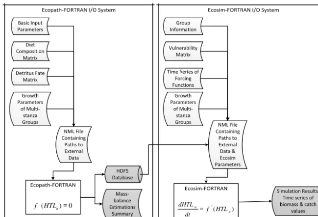
it in future versions. A schematic view of the EwE-F com-ponents and the input/output (I/O) files necessary for infor-mation exchange are given in Fig. 1. In the following two sections (3.1 and 3.2), the structure and functioning of the components in Fig. 1 are described in detail.
3.1 Ecopath-F
Ecopath-F is the component of EwE-F that carries out mass-balance calculations given in Eq. (1). Similar to stock Eco-path, it requires the same fundamental input parameters to be entered via four tab-delimited ASCII (American Standard Code for Information Interchange) encoded text input files: (i) a scenario file containing the basic input and multi-stanza parameters and catches, (ii) a file comprising the diet com-position matrix of the state variables, (iii) a file compris-ing the detritus fate of the state variables and, (iv) if appli-cable, a file including the growth parameters of the multi-stanza groups. Furthermore, Ecopath-F requires a Fortran “namelist” file that includes the full paths and names of the above-mentioned four input files and, in addition, the path and name of the output HDF5 (Hierarchical Data Format version 5, www.hdfgroup.org/HDF5) file which the mass-balance calculation results will be output to and which will be used to initialise and run Ecosim-F (Fig. 1).
An Ecopath-F run produces two output files: (i) an ASCII file which includes the summary of estimated parameters and basic statistical information, and (ii) an HDF5 file specifically formatted to define the initial conditions for the Ecosim-F simulation (Fig. 1). The output HDF5 file includes all the parametric details about the state variables of the Eco-path run and furthermore comprises the diet composition ma-trix, detritus fate matrix and multi-stanza group parameters.
Ecopath-F is independent of the Ecosim-F implementa-tion; however, Ecosim-F requires output data from Ecopath-F plus additional parameter settings. The data transfer from Ecopath-F to Ecosim-F is carried out via the intermediary HDF5 data file.
3.2 Ecosim-F
Ecopath-FORTRAN I/O System Ecosim-FORTRAN I/O System
Ecosim-FORTRAN Ecopath-FORTRAN
NML File Containing
Paths to External Data Basic Input
Parameters
Diet Composition
Matrix
Detritus Fate Matrix
Growth Parameters
of Multi-stanza Groups
HDF5 Database
Mass-balance Estimations
Summary
NML File Containing
Paths to External Data & Ecosim Parameters Group
Information
Vulnerability Matrix
Time eries of Forcing Functions Growth Parameters
of Multi-stanza Groups
Simulation Results: Time series of biomass & catch
values )
(
'' n n
HTL f dt dHTL
0 ) (HTLn
f
S
Figure 1. The EwE-F data input/output scheme. Curved white rectangular boxes denote tab-delimited ASCII files providing external data input to the EwE-F models (rectangles). Curved grey-shaded rectangles and the cylindrical box denote the model output via tab-delimited ASCII and HDF5 files respectively. For details see Sect. 3.1 and 3.2.
in years, to prepare the Ecosim simulation (for details, see Christensen et al., 2005, p. 78; Akoglu et al., 2015).
Once completed, Ecosim-F simulation produces five tab-delimited ASCII coded text files comprising the annual and monthly absolute and relative biomass values of the state variables and a file comprising monthly catches of the fished state variables throughout the simulation in the model direc-tory (Fig. 1).
3.3 The skill assessment of EwE-F
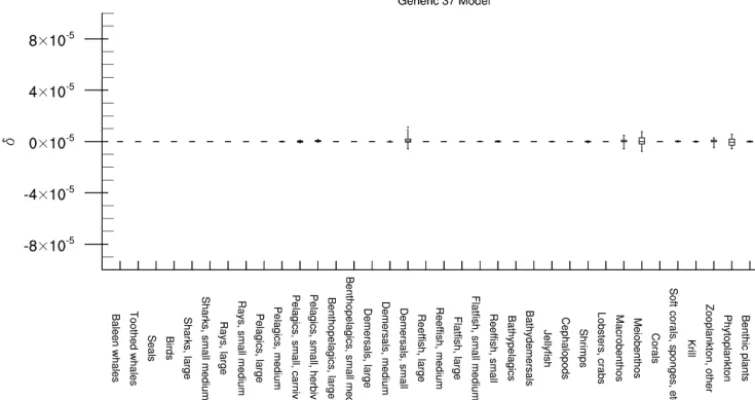
In order to assess the skill of EwE-F with respect to EwE, two test case simulations, Generic 37 and Tampa Bay, which are distributed with the installation of the EwE software, were used. The test case simulations were run both with EwE ver-sion 6.5 and EwE-F verver-sion 1.0 and the residuals between simulated absolute biomasses of state variables were used to evaluate the performance of EwE-F. It is worth noting that other EwE versions may produce slightly different results compared to EwE-F v1.0. The residuals for each state vari-able in the respective simulations were visualised with box-whisker plots showing the minimum value, 25th percentile, median, 75th percentile and maximum values respectively (Figs. 2 and 3).
The residuals between the simulated biomass values of EwE-F and EwE ranged from 10−8to 10−5, with the maxi-mum difference found to be of the order of 10−5. The resid-uals calculated from the comparison of the simulations con-firmed that EwE-F possessed the necessary skill to reproduce the results of EwE for the Generic 37 and Tampa Bay simu-lations. The magnitude of the misfits concluded that EwE-F
was capable of being used in conjunction with other models without introducing significant sources of error to the result-ing modellresult-ing scheme.
4 Exploring EwE-F flexibilities: example from a complex coupling exercise
The Fortran recoding of EwE creates great flexibility for customisation, modification or coupling to different models written in Fortran. An example, which illustrated the poten-tial of such flexibility, came from the integration of EwE-F with a biogeochemical Fortran model. In fact, the direct inte-gration of these two models required one to address and sub-sequently solve a number of problems. These included defin-ing the links between the two models and modifydefin-ing them accordingly, exchanging information between the two mod-els, dealing with different model time steps, and accounting for different model currencies.
Figure 2. The residuals between absolute biomasses simulated by EwE 6.5 and EwE-F 1.0 for the Generic 37 model.xaxis denotes all state variables in the model.
Figure 3. The residuals between absolute biomasses simulated by EwE 6.5 and EwE-F 1.0 for the Tampa Bay model.xaxis denotes all state variables in the model.
is wet weight. The time step of the model is 1 month, the default time step of the EwE software.
The biogeochemical model is a Fasham-like (Fasham et al., 1990) 0-D box model of the northern Adriatic Sea (Cos-sarini and Solidoro, 2008) and consists of phytoplankton, zooplankton, and heterotrophic bacteria groups, one pool of inorganic phosphorus (PO34−), one dissolved organic mat-ter compartment in mat-terms of phosphorus (DOP) and carbon (DOC), and one particulate organic matter compartment in terms of phosphorus (POP) and carbon (POC) (Fig. 4). The model is a multi-currency model calculating the biomasses of its particular state variables (sediment, dissolved organic matter, particulate organic matter) both in terms of carbon
and phosphorus. The time step of the model is 1 h. A full de-scription of the biogeochemical model is given in Cossarini and Solidoro (2008).
EwE-F
LTL
DOC POC
Sediment (C)
Detritus (P)
Detritus (P) Bacteria (P)Bacteria (P) Phyto (P)Phyto (P) Zoo (P)Zoo (P) Zoobenthos
(P) Fish (P)
Birds (P) Mammals (P)
Sediment
(P) PO4 POP DOP Bacteria (C) Phyto (C) Zoo (C)
x RPC x RPC
Predation Excretion Mortality
Fisheries
x RPC
Figure 4. Coupled trophodynamic model scheme of the Gulf of Trieste (northern Adriatic Sea) showing the linkages between the HTL and LTL models. Phosphorus (denoted with P) was used as the currency for all of the HTL state variables and flows linking the two models. Flows originating from the state variables of the LTL model to the HTL model, which were expressed in carbon (denoted with C), i.e. phytoplankton and zooplankton, were converted to phosphorus (by multiplying variable-specific phosphorus-to-carbon (RPC) ratios) before being transferred. Grey-shaded state variables and flows in the HTL model were replaced by the LTL model’s corresponding state variables and the new linked flows are shown in black dashed and continuous lines. Abbreviations: Zoo (small and large zooplankton groups), Phyto (small and large phytoplankton groups), PO4(phosphate), POP (particulate organic phosphorus), and DOP (dissolved organic phosphorus).
the biogeochemical model, i.e. plankton groups plus inor-ganic and orinor-ganic nutrient forms (Fig. 4). For simplicity, the HTL and LTL groups are not given in detail in the figure; however, sources and sinks of the whole HTL compartment and the linkages between the HTL and LTL domains and state variables are shown.
The second step in the harmonisation of models consisted of accounting for the different currencies used. Consider-ing the multiple currency utilisation of the biogeochemical model for some of its state variables and the fact that the ap-plication of a similar principle in the HTL model would re-quire the modification of the various calculations in the state equation of the original EwE software, the state variables of the HTL model, which were in wet weight (tons), were con-verted to phosphorus (µmol P) weight utilising C:N:P ratios taken from the literature.
The third step in the harmonisation procedure was to rec-oncile the differences in the integration time step between the two models. Considering that the biogeochemical model con-sisted of state variables with faster dynamics compared to the HTL model, it was convenient to make the HTL model com-ply with the integration step of the biogeochemical model. For this purpose, the rates of the HTL model, which were “per year (yr−1)”, were converted to “per hour (h−1)” by simply dividing the rates by 8760 (365 d−1×24 h−1)so that
the HTL variables could be integrated with the same time step of the biogeochemical model.
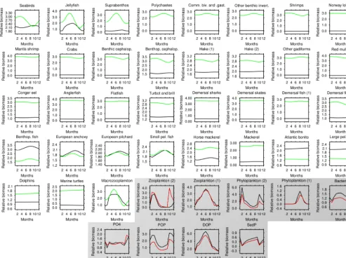
The final step in the harmonisation process would be to adjust the closure terms of the biogeochemical model (mor-tality rates of zooplankton and phytoplankton groups) so as to compensate for the additional losses through explicit pre-dation of these groups by the HTL state variables. However, for our specific application, we decided to keep these values identical to the standalone biogeochemical model, as the cou-pled model produced similar seasonal cycles observed in the standalone biogeochemical model except the missing second cycle in mesozooplankton (Fig. 6) and as our aim was in-deed to have plankton dynamics qualitatively comparable to the biogeochemical model.
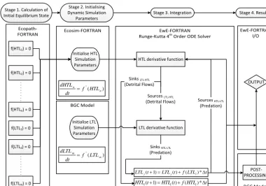
Ecosim-FORTRAN EwE-FORTRAN
Runge-Kutta 4th
Order ODE Solver Ecopath-FORTRAN BGC Model BGC Model EwE-FORTRAN I/O
HTL derivative function
LTL derivative function f(HTL1) = 0
f(HTL2) = 0
f(HTLn) = 0
f(LTL1) = 0
f(LTL2) = 0
f(LTLm) = 0
Initialise HTL Simulation Parameters Initialise LTL Simulation Parameters Stage 1. Calculation of
Initial Equilibrium State
Stage 2. Initialising Dynamic Simulation
Parameters
Stage 3. Integration
t LTL f t LTL t
LTLj(1) j() ( i)*
t HTL f t HTL t
HTLi(1) i() ( i)* Sinks HTL-LTL
(Predation) Sinks LTL-HTL
(Detrital Flows)
POST-PROCESSING
OUTPUT
Sources HTL-LTL
(Predation)
Stage 4. Results
Sources LTL-HTL
(Detrital Flows) ) ( '' m m LTL f dt dLTL ) ( '' n n HTL f dt dHTL
Figure 5. The technical overview of the coupling scheme. ODE stands for “ordinary differential equation”, I/O stands for “input/output”, and BGC stands for “biogeochemical model” used in the present work.
which were necessary to perform a dynamic simulation af-ter completing all of the harmonisation steps. In the second stage, utilising the calculations from the previous stage, the HTL and LTL models were initialised by calculating initial conditions for each of their respective state variables util-ising their specific internal routines. In the third stage, the sources and sinks of HTL and LTL state variables were com-puted by utilising their respective derivative functions during the whole simulation period. The selection of the derivative function to be used to calculate the differentials of the state variables depended on the rank of the state variables deter-mined during the Ecopath-F set-up in the first stage. This stage continued iteratively until the end of the simulation and, at the end of each time step, the fourth stage was ex-ecuted so that the results calculated at each time step were, if required, post-processed and then written to the results files. Post-processing of LTL results might not be necessary in all cases, but only if the LTL model is a multi-currency model and calculates its variables in more than one currency. In our example, because the LTL model represented some of its state variables both in carbon and phosphorus but the cou-pled HTL model only in phosphorus, a post-processing step was necessary to compute the corresponding phosphorus val-ues of variables that were in carbon units while interchang-ing information between the HTL and LTL derivative func-tions as well as before writing the results into the output files. The coupled simulation was run for 10 years, two of which
were for spin-off. In the simulations, we used default val-ues for vulnerabilities (vij=2) that represent a mixed
con-trol (Christensen et al., 2005).
Figure 6. Monthly results of the final year in a 10-year simulation of the coupled (black lines) model versus simulations of uncoupled EwE 6.5 (green lines for HTL variables – unshaded boxes) and uncoupled biogeochemical (red lines for LTL variables – grey shaded boxes) models.
into the coupled scheme, pelagic-associated state variables increased due to the explicit representation of resuspension of detritus and remineralisation that favoured plankton. Thus, as shown in Fig. 6, the consequences of two-way coupling were not only one-directional. These proved that the proper exchange of information and the establishment of successful interaction between the two models were realised in the final coupled scheme.
5 Discussions
5.1 Potential and flexibility of the application
In this work, the reliability of EwE-F was proven by utilising two sample models as test cases and comparing the absolute biomass values simulated by EwE-F against the simulated absolute biomass values by stock EwE version 6.5. Further-more, the applicability of EwE-F in an E2E modelling
frame-work was exemplified with a test case for the Gulf of Trieste ecosystem. This example proved the adaptability of EwE-F for coupled modelling frameworks, facilitating its integra-tion with other hydrodynamic and biogeochemical Fortran models for aquatic ecosystems in ecosystem research. The scheme used in this work successfully conveyed two-way dynamics of HTL and LTL domains along the whole food web. As a step forward, this opened up the opportunity for using EwE, by utilising EwE-F implementation, as an HTL component of holistic ecosystem representations in various ecosystems.
EwE-F
D) Biogeochemical model
A) Socioeconomic model C) Population dynamics
model B) Bioenergetics model
Fleet
Somatic processes Reproductive processes
DOC POC
Sediment (C)
Detritus (P)
Detritus (P) Bacteria (P)Bacteria (P) Phyto (P)Phyto (P) Zoo (P)Zoo (P) Zoobenthos
(P) Fish (P)
Birds (P) Mammals (P)
Sediment
(P) PO4 POP DOP Bacteria (C) Phyto (C) Zoo (C)
Fisheries Landings
Market
Fishing Effort Human
Population
Trawlers Seiners
Zoobenthos
Respiration Feces
Larvae
Fry
Juvenile
Eggs
Growth process
Eggs
Reserve Outflow
Fish (P)
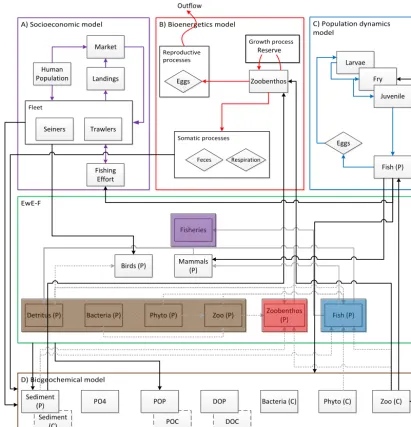
Figure 7. Potentialities provided by the EwE-F approach. Coloured arrows denote flows specific to the integrating Fortran models. Black arrows denote linking flows and grey-shaded arrows denote flows replaced/augmented by the linking flows. Boxes denoted by the letters A, B, C and D and bordered by coloured lines replace the respective colour-shaded regions in the EwE-F box (bordered green) under the coupling/integration scheme.
2013) via its simplistic but ecologically capable approach to form E2E representations of aquatic ecosystems through the incorporation of EwE-F. In addition, the EwE-F enables sig-nificant opportunities for integrating it with any kind of For-tran model as depicted in Fig. 7. The figure represents a typ-ical EwE food web model in the middle rectangular box and elaborates the possibilities of modifying EwE-F in different ways by replacing different components with sophisticated model representations for selected state variables or incorpo-rating additional Fortran models to enhance the applicability of the original EwE approach. These solutions and possibil-ities are explored in detail in the following sections: (i)
rec-onciling different integration steps (Sect. 5.1.1), (ii) deal-ing with models that use multiple currencies (Sect. 5.1.2), and (iii) other possibilities: incorporation of population de-mographic structure, physiological processes, and socioeco-nomic frameworks (Sect. 5.1.4).
5.1.1 Reconciling different integration steps
turnover rate) and vice versa when exchanging information (time-averaged coupling), and (ii) utilising a common inte-grator for both models and adjusting the rates of the model with slower dynamics to comply with the time window of the model with faster dynamics (real-time coupling). Although Ecosim, by default, works with monthly time steps, it is ca-pable of simulating high-frequency dynamics using shorter time steps. In the present work, we opted for the latter to showcase the possibility of harmonisation in terms of inte-gration step size when using EwE-F in coupled modelling schemes. The difference in the time resolution of both mod-els was remedied by adjusting the HTL model’s time step (1 month) to conform to the time step of the biogeochemical model (1 h) in order to render the use of one common or-dinary differential equation (ODE) solver (the Runge–Kutta fourth-order) possible. Furthermore, due to this change in the time step of the HTL model, the annual rates of the HTL groups were converted to hourly rates by simple arithmetic calculations.
5.1.2 Dealing with models that use multiple currencies Some biogeochemical models may carry out their computa-tions in more than one currency for explicit representation of the ratios of fundamental nutrients in the system and their rate limiting conditions on nutrient uptake and primary pro-ductivity that can vary in space and time. The multiple cur-rency approach, however, is usually not applied in HTL mod-els, although implicit nutrient-based limitations can be repre-sented in EwE (Araújo et al., 2006; Christensen et al., 2005). Hence, the coupling exercise presented here provided a sim-ple solution for such situations. In order to reconcile the cur-rency differences, one may opt to pick one of the currencies utilised in the biogeochemical model as the one considered to be the limiting nutrient, use it for the final coupled scheme incorporating the EwE-F model, and post-process the deriva-tive function outputs of the two models when exchanging in-formation. In the coupling example given in this work, the difference in the currencies of the models was adjusted by converting the currency of the HTL model from wet weight to phosphorus (P) by utilising the conversion rates and equa-tions available in the literature for HTL groups (stage 1 of the coupling scheme in Fig. 5). In addition, the simulated results of the biogeochemical model (which were in dual currency, phosphorus and carbon) were post-processed prior to output and transferred to EwE-F so as to comply with the currency of the HTL compartment (stage 4 in Fig. 5). The approach used in this work proved to be a practical solution for the is-sue in cases where there is no particular consideration to have simultaneously tracking multiple currencies in the HTL food web. However, with the availability of EwE-F, HTL models with computations of multiple model currencies can even be set up if desired, although this will require significant modi-fication of various calculations in the EwE state equations.
5.1.3 Spatial simulations
Given the current experience with biogeochemical models coupled to hydrodynamic models (e.g. Lazzari et al., 2012), explicit accounting for spatial variability is important for any assessment of marine ecosystem dynamics. Future ef-forts are required to add spatial simulation capabilities to EwE-F, either by implementing Ecospace in Fortran or by direct integration of Ecosim-F in a spatially explicit coupled hydrodynamic–biogeochemical model. This planned future work could lead EwE-F to play a substantial role in spatial simulations.
5.1.4 Other possibilities: population demographic structure, physiological processes, socioeconomic frameworks
Similar to the flexibility of EwE provided by its plug-in system, EwE-F gives broad possibilities for interconnecting HTL models with other Fortran models sophisticating and/or incorporating HTL processes. Examples span from fish pop-ulation to socioeconomic dynamic models.
For instance, EwE-F permits incorporating sophisticated population dynamic models written in Fortran within the EwE-F scheme (Fig. 7c). These population models can be of any kind, including a population’s demographic structure (age–size classes) used for stock assessment and to account for differences in fecundity by ages or size (Hilborn and Wal-ters, 1992).
Moreover, EwE-F allows for parameterising various rates for HTL groups (e.g. assimilation efficiency, respiration) un-der the influence of various environmental factors (e.g. tem-perature, pH, light) that is not always straightforward oth-erwise (Fig. 7d). In addition, EwE-F allows for replacing the growth of certain state variables in the food web with sophisticated bioenergetics models coded in Fortran. In this way, various physiological processes of the selected HTL or-ganisms can be related directly and explicitly to the ambi-ent physical factors such as light, temperature and nutriambi-ent availability (Fig. 7b). With EwE-F, in fact, as demonstrated in this work, the dynamics of any desired additional state variable in the final coupled scheme could be resolved using derivative functions defined in other models during run-time. This allows for a two-way coupling of, potentially, any num-ber of models (including earth system ones) in one coupling scheme.
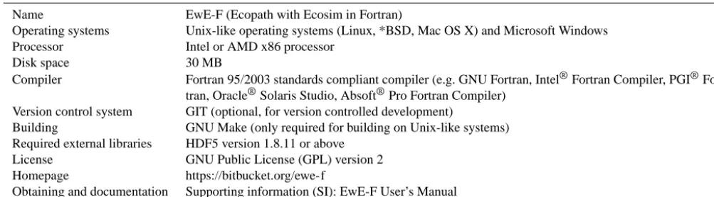
Table 1. General system and software related requirements of EwE-F v1.0.
Name EwE-F (Ecopath with Ecosim in Fortran)
Operating systems Unix-like operating systems (Linux, *BSD, Mac OS X) and Microsoft Windows Processor Intel or AMD x86 processor
Disk space 30 MB
Compiler Fortran 95/2003 standards compliant compiler (e.g. GNU Fortran, Intel®Fortran Compiler, PGI® For-tran, Oracle®Solaris Studio, Absoft®Pro Fortran Compiler)
Version control system GIT (optional, for version controlled development)
Building GNU Make (only required for building on Unix-like systems) Required external libraries HDF5 version 1.8.11 or above
License GNU Public License (GPL) version 2 Homepage https://bitbucket.org/ewe-f
Obtaining and documentation Supporting information (SI): EwE-F User’s Manual
5.2 Other practical considerations and future development
In contrast to the EwE, the introduction of namelist and HDF5 files to be used for the operation of EwE-F may cre-ate a hindrance to its users. However, it is not necessarily more complicated than the current EwE database files (MS Access). EwE-F requires an HDF5 database file only when transferring information from Ecopath-F to Ecosim-F, and output to and input from this file does not require any user intervention. In addition, the results of both Ecopath-F and Ecosim-F models are output into TAB-delimited ASCII files, which are quite similar to the EwE’s output files, i.e. comma-separated value (CSV) ASCII files. These files can easily be opened with spreadsheet programs. The only hindrance for the user could be the preparation of the TAB-delimited ASCII input files for Ecopath-F and Ecosim-F, which how-ever is explained in the User’s Manual in detail. On the other hand, through this simple input/output scheme utilising ASCII encoded text files, the availability of EwE-F provides a further opportunity by giving Fortran modellers the possi-bility to perform detailed sensitivity and uncertainty analyses using hundreds of ensemble scenarios that can easily be pre-pared also by using modern high-level languages (e.g. Perl, Python, NCL) in addition to Fortran. For their convenience, users of EwE-F are advised to set up, test and fit their mod-els to time series data using EwE, also benefiting from the several routines included in EwE, and, thereafter, to transfer their models to EwE-F.
Ecospace (Walters et al., 1999) and other complemen-tary routines aforementioned (see Sect. 3) were not imple-mented considering that EwE-F was not designed to be an EwE replacement but a bare-bones incarnation that can be used easily for purposes summarised in Sect. 5.1.4. There-fore, analyses requiring the aforementioned specific routines (e.g. Monte Carlo analysis, network analysis, etc.) in uncou-pled or couuncou-pled EwE-F simulations can be done by coding the required specific routines or, alternatively, EwE could be employed for such purposes. The current lack of such
use-ful tools that are present in EwE 6.5 is considered to be a drawback for EwE-F v1.0, which may represent an obstacle for some users. However, these technical shortcomings and the lack of these tools including mediation function and time series fitting via vulnerability parameter search are planned to be addressed in the future by incorporating these rou-tines into EwE-F and developing a Visual Basic plug-in for stock EwE which will prepare input files required by EwE-F through EwE’s graphical user interface in a straightforward way. Furthermore, considering advancements in coupling on the spatial scale, future efforts in developing EwE-F may also focus on incorporating 2-D spatial dynamics by implement-ing the Ecospace module of EwE to facilitate the use of EwE-F in schemes that require spatial–temporal dynamics to be resolved.
Another important consideration to be discussed is to keep EwE-F on par with EwE. With every new release of EwE software, many things are prone to change. However, the ma-jority of these changes are related to the ancillary functional-ities (graphical user interface, network analysis routines, etc., but not the core state equations and their related calculations) that are not included in EwE-F. Furthermore, the changes to the basic model structure and dynamics have remained al-most unchanged since EwE version 5. Hence, it is believed that the core structure of EwE-F (state equations and other re-lated calculations) can be kept on par with the original EwE with little effort, considering that the development of EwE-F is a joint effort of two prominent marine science institutes and is not strictly bound to any individual.
6 Conclusions
to demonstrate the feasibility of the approach, and it does not mean that EwE-F can be applied only in E2E modelling frameworks. As discussed in Sect. 5.1.4, many other uses of EwE-F are possible.
EwE-F is still in its infancy and future development ef-forts will focus on maturing the software and implementing missing useful features like times series fitting via vulnera-bility search, capavulnera-bility to define multiple fishing fleets and explicit spatial simulation. We believe that the development pace of EwE-F will accelerate with the adoption and utilisa-tion of the software in the scientific community.
Code availability
The source code of EwE-F version 1.0 detailed in the present work and the corresponding User’s Manual can be obtained as a supplement to this article. In the User’s Manual, detailed instructions to obtain the current and future versions of EwE-F along with building and running EwE-EwE-F on different plat-forms are described. Further versions of the EwE-F model and their respective documentations can be obtained at bit-bucket.org (https://bitbit-bucket.org/ewe-f). The system require-ments, license and other basic information regarding EwE-F version 1.0 are given in Table 1.
The Supplement related to this article is available online at doi:10.5194/gmd-8-2687-2015-supplement.
Acknowledgements. The authors would like to thank Gianpiero Cossarini and Paolo Lazzari (ECHO group, Oceanography Di-vision, OGS), Villy Christensen and Jeroen Steenbeek (Ecopath Research and Development Consortium) for comments and discussions, and Marta Coll (IRD) for permitting the update and use of the Adriatic EwE model. The authors would like to acknowledge support from EU FP 7 projects MEECE (Marine Ecosystem Evolution in a Changing Environment, www.meece.eu), PERSEUS (Policy-oriented Marine Environmental Research for the Southern European Seas, http://www.perseus-net.eu/), and OPEC (Operational Ecology, http://marine-opec.eu/), and the support of the Italian RITMARE Flagship Project – The Italian Research for the Sea – coordinated by the Italian National Research Council and funded by the Italian Ministry of Education, University and Research within the National Research Program 2011–2013. This work was facilitated by the support of the International Centre for Theoretical Physics (ICTP) Training and Research in Italian Laboratories (TRIL) programme with a grant provided to Ekin Akoglu. This work is also a contribution to the endeavours carried out under the Ecopath Research and Development Consortium (www.ecopath.org/consortium).
Edited by: S. Valcke
References
Adcroft, A., Campin, J. M., Hill, C., and Marshall, J.: Implemen-tation of an atmosphere-ocean general circulation model on the expanded spherical cube, Mon. Weather Rev., 132, 2845–2863, 2004.
Ahrens, R. N. M., Walters, C. J., and Christensen, V.: Forag-ing arena theory, Fish Fish., 13, 41–59, doi:10.1111/j.1467-2979.2011.00432.x, 2012.
Akoglu, E., Libralato, S., Salihoglu, B., Oguz, T., and Solidoro, C.: The EwE-F User’s Manual for version 1.0. August 2015, Trieste-Italy, 73 pp., 2015.
Araújo, J. N., Mackinson, S., Stanford, R. J., Sims, D. W., South-ward, A. J., Hawkins, S. J., Ellis, J. R., and Hart, P. J. B.: Mod-elling food web interactions, variation in plankton production, and fisheries in the western English Channel ecosystem, Mar. Ecol. Prog. Ser., 309, 175–187, 2006.
Backus, J. W., Stern, H., Ziller, I., Hughes, R. A., Nutt, R., Beeber, R. J., Best, S., Goldberg, R., Haibt, L. M., Herrick, H. L., Nelson, R. A., Sayre, D., and Sheridan, P. B.: The FORTRAN Automatic Coding System, Western joint computer conference: Techniques for reliability (Los Angeles, California: Institute of Radio Engi-neers, American Institute of Electrical EngiEngi-neers, ACM), 188– 198, doi:10.1145/1455567.1455599, 1957.
Beecham, J. A., Bruggeman, J., Aldridge, J. N., and Mackinson, S. P.: Linking Biogeochemical and Upper Trophic Level Models using an XML based Semantic Coupler, ICES CM 2010/ Session L, 2010.
Blackford, J. C., Allen, J. I., and Gilbert, F. J.: Ecosystem dynamics at six contrasting sites: a generic modelling study, J. Mar. Syst., 52, 191–215, doi:10.1016/j.jmarsys.2004.02.004, 2004. Blumberg, A. F. and Mellor, G. L.: A coastal ocean numerical
model, in Mathematical Modelling of Estuarine Physics, Proc. Int. Symp., Hamburg, Aug. 1978, edited by: Sunderman, J. and Holtz, K.-P., Springer-Verlag, Berlin, 203–214, 1980.
Christensen, V. and Walters, C. J.: Ecopath with Ecosim: methods, capabilities and limitations, Ecol. Model., 172, 109–139, 2004. Christensen, V., Walters, C. J., and Pauly, D.: Ecopath with
Ecosim: A User’s Guide, Fisheries Centre, University of British Columbia, Vancouver, Canada, 154 pp., 2005.
Christensen, V., Coll, M., Piroddi, C., Steenbeek, J., Buszowski, J., and Pauly, D.: A century of fish biomass decline in the ocean. Mar. Ecol. Prog. Ser., 512, 155–166, doi:10.3354/meps10946, 2014.
Coll, M., Santojanni, A., Palomera, I., Tudela, S., and Arneri, E.: An ecological model of the Northern and Central Adriatic Sea: Anal-ysis of ecosystem structure and fishing impacts, J. Mar. Syst., 67, 119–154, 2007.
Cossarini, G. and Solidoro, C.: Global sensitivity analysis of a trophodynamic model of the Gulf of Trieste, Ecol. Modell., 212, 16–27, 2008.
Fasham, M. J. R., Ducklow, H. W., and McKelvie, S. M.: A nitrogen-based model of plankton dynamics in the oceanic mixed layer, J. Mar. Res., 48, 591–639, 1990.
Fulton, E. A.: Approaches to end-to-end ecosystem models, J. Mar. Syst., 81, 171–183, 2010.
Kearney, K. A., Stock, C., Aydin, K., and Sarmiento, J. L.: Coupling planktonic ecosystem and fisheries food web models for a pelagic ecosystem: description and validation for the subarctic Pacific, Ecol. Modell., 237, 43–62, 2012.
Lazzari, P., Solidoro, C., Ibello, V., Salon, S., Teruzzi, A., Béranger, K., Colella, S., and Crise, A.: Seasonal and inter-annual vari-ability of plankton chlorophyll and primary production in the Mediterranean Sea: a modelling approach, Biogeosciences, 9, 217–233, doi:10.5194/bg-9-217-2012, 2012.
Libralato, S., and Solidoro, C.: Bridging biogeochemical and food web models for an End-to-End representation of marine ecosys-tem dynamics: The Venice lagoon case study, Ecol. Modell., 220, 2960–2971, 2009.
Madec, G.: NEMO ocean engine, Note du Pôle de modélisation, Institut Pierre-Simon Laplace (IPSL), France, No 27 ISSN No 1288–1619, 2008.
Neumann, T.: Towards a 3d-ecosystem model of the Baltic Sea, J. Mar. Syst., 25, 405–419, 2000.
Rose, K. A., Allen, J. I., Artioli, Y., Barange, M., Blackford, J., Carlotti, F., Cropp, R., Daewel, U., Edwards, K., Flynn, K., Hill, S. L., HilleRisLambers, R., Huse, G., Mackinson, S., Megrey, B., Moll, A., Rivkin, R., Salihoglu, B., Schrum, C., Shannon, L., Shin, Y.-J., Smith, S. L., Smith, C., Solidoro, C., St. John, M., and Zhou, M.: End-To-End Models for the Analysis of Ma-rine Ecosystems: Challenges, Issues, and Next Steps, Mar. Coast. Fish., 2, 115–130, 2010.
Salihoglu, B., Neuer, S., Painting, S., Murtugudde, R., Hofmann, E. E., Steele, J. H., Hood, R. R., Legendre, L., Lomas, M. W., Wig-gert, J. D., Ito, S., Lachkar, Z., Hunt Jr., G. L., Drinkwater, K. F., and Sabine, C. L.: Bridging marine ecosystem and biogeochem-istry research: Lessons and recommendations from comparative studies, J. Mar. Syst., 109, 161–175, 2013.
Shchepetkin, A. F. and McWilliams, J. C.: The regional oceanic modeling system (ROMS): a split-explicit, free-surface, topography-following-coordinate oceanic model, Ocean Model., 9, 347–404, 2005.
Steele, J. H.: Assessment of some linear food web models, J. Mar. Syst., 76, 186–194, 2009.
Stock, C. A., Dunne, J. P., and John, J. G.: Global-scale carbon and energy flows through the marine planktonic food web: An analy-sis with a coupled physical–biological model, Progr. Oceanogr., 120, 1–28, 2014.
Ulanowicz, R. E.: Growth and Development: Ecosystem Phe-nomenology. Springer Verlag (reprinted by iUniverse, 2000), New York, 203 pp., 1986.
Vichi, M., Cossarini, G., Gutierrez Mlot, E., Lazzari, P., Lovato, T., Mattia, G., Masina, S., McKiver, W., Pinardi, N., Solidoro, C., and Zavatarelli, M.: The Biogeochemical Flux Model (BFM): Equation Description and User Manual. BFM version 5.1. BFM Report series N. 1. March 2015, Bologna, Italy, 89 pp., 2015. Walters, C., Christensen, V., and Pauly, D.: Structuring dynamic
models of exploited ecosystems from trophic mass-balance as-sessments, Rev. Fish Biol. Fish., 7, 139–172, 1997.
Walters, C. J., Pauly, D., and Christensen, V.: Ecospace: Prediction of mesoscale spatial patterns in trophic relationships of exploited ecosystems, with emphasis on the impacts of marine protected areas, Ecosystems, 2, 539–554, 1999.