A flexible importance sampling method for integrating subgrid processes

www.geosci-model-dev.net/9/413/2016/ doi:10.5194/gmd-9-413-2016

© Author(s) 2016. CC Attribution 3.0 License.

A flexible importance sampling method for integrating

subgrid processes

E. K. Raut and V. E. Larson

University of Wisconsin – Milwaukee, Department of Mathematical Sciences, Milwaukee, WI, USA

Correspondence to: E. K. Raut ([email protected])

Received: 17 August 2015 – Published in Geosci. Model Dev. Discuss.: 22 October 2015 Revised: 20 December 2015 – Accepted: 15 January 2016 – Published: 29 January 2016

Abstract. Numerical models of weather and climate need to compute grid-box-averaged rates of physical processes such as microphysics. These averages are computed by integrat-ing subgrid variability over a grid box. For this reason, an important aspect of atmospheric modeling is spatial integra-tion over subgrid scales.

The needed integrals can be estimated by Monte Carlo in-tegration. Monte Carlo integration is simple and general but requires many evaluations of the physical process rate. To re-duce the number of function evaluations, this paper describes a new, flexible method of importance sampling. It divides the domain of integration into eight categories, such as the tion that contains both precipitation and cloud, or the por-tion that contains precipitapor-tion but no cloud. It then allows the modeler to prescribe the density of sample points within each of the eight categories.

The new method is incorporated into the Subgrid Im-portance Latin Hypercube Sampler (SILHS). The resulting method is tested on drizzling cumulus and stratocumulus cases. In the cumulus case, the sampling error can be con-siderably reduced by drawing more sample points from the region of rain evaporation.

1 Introduction

Coarse-resolution atmospheric models of weather and cli-mate do not solve differential equations; they solve integro-differential equations, that is, equations containing both derivatives and integrals. Although a derivation of an at-mospheric model starts with differential equations, such as the Navier–Stokes or advection–diffusion equations, those equations are coarse-grained or filtered before being

dis-cretized (e.g., Leonard, 1974; Pope, 2000). Typically, a spa-tial running-mean filter is used, producing equations simi-lar to Reynolds-averaged equations (e.g., Germano, 1992). Each term in the filtered equations is spatially averaged over a grid box. For instance, in a prognostic equation for grid-averaged rain mixing ratio, the grid-grid-averaged rain is updated by grid-averaged microphysical process rates. Schemati-cally, we may give an example of such a filtered equation: ∂r¯

∂t = ¯h+. . ., (1)

wherer¯ denotes grid-averaged rain mixing ratio,t denotes time, and h¯ denotes the grid-averaged microphysical time tendency of rain mass mixing ratio. Because a grid-box av-erage is an integral (divided by the grid-box volume), the re-sulting filtered equations are integro-differential equations. Therefore, a central problem in atmospheric modeling is (subgrid-scale, spatial) integration.

Mathematically, the problem is to evaluate integrals of the form

¯ h≡

Z

h(x)P (x)dx, (2)

The integrals also need to be computed for each grid column in the horizontal and each grid level in the vertical.

To carry out this integration (i.e., “quadrature”), re-searchers have proposed several methods. First, the inte-gral (Eq. 2) may be evaluated analytically (e.g., Zhang et al., 2002; Larson and Griffin, 2006; Morrison and Gettelman, 2008; Cheng and Xu, 2009; Griffin and Larson, 2013; Lar-son and Griffin, 2013; Lebsock et al., 2013; Boutle et al., 2014). Analytic integration has the advantage of accuracy, but it can be carried out only if both the process rateh(x) and the subgrid-scale PDFP (x)are sufficiently simple. Fur-thermore, analytic integration is carried out grid level by grid level, and does not compute the vertical overlap of cloud properties. Vertical overlap is related to the correlation be-tween quantities at two points in space, one located directly above the other. The degree of vertical overlap has a strong influence on, e.g., radiative transfer. Second, the integrals may be computed by deterministic quadrature (Xiu, 2009; Golaz et al., 2011; Chowdhary et al., 2015). Deterministic quadrature solves an integral by computing a weighted sum of integrand values evaluated at specially chosen quadrature points. Deterministic quadrature has a couple of advantages: unlike analytic integration, deterministic quadrature is appli-cable to a broad range of processes, and like analytic inte-gration, deterministic quadrature is still accurate. Determin-istic quadrature also has a disadvantage: it does not com-pute vertical overlap. Third, the integrals can be evaluated by Monte Carlo integration (e.g., Gentle, 2003; Kalos and Whitlock, 2008). In Monte Carlo integration, random sam-ples are drawn from the subgrid PDFP (x), the integrand is evaluated at each sample point, and the resulting values are suitably averaged. Monte Carlo integration is broadly appli-cable and can be configured to model vertical overlap (Barker et al., 2002, 2008; Pincus et al., 2003, 2006; Räisänen et al., 2004, 2005, 2007, 2008; Räisänen and Barker, 2004; Lar-son et al., 2005; LarLar-son, 2007; Hill et al., 2011; LarLar-son and Schanen, 2013; Tonttila et al., 2013, 2015). However, Monte Carlo integration converges slowly. Obtaining an accurate in-tegration requires many costly evaluations of a microphysics parameterization.

To improve the convergence of Monte Carlo integration, many methods have been proposed. Two broad strategies are stratified sampling and importance sampling (Press et al., 2007; Lemieux, 2009). Stratified sampling spreads out the sample points in sample space in order to avoid clumping, which leads to poor sampling. One popular stratified sam-pling method is Latin hypercube samsam-pling, which stratifies along each dimension of the integral (e.g., McKay et al., 1979; Owen, 2003). Another strategy, importance sampling, preferentially places sample points in important regions of the integration domain (Press et al., 2007; Lemieux, 2009). For instance, extra sample points may be placed within cloud because that is where important processes occur, such as the formation and growth of cloud droplets.

Some sampling methods combine stratified and impor-tance sampling. For insimpor-tance, a prior version of the Sub-grid Importance Latin Hypercube Sampler (SILHS) placed sample points preferentially in cloud, and also stratified the within-cloud sample points using Latin hypercube sampling (Larson et al., 2005; Larson and Schanen, 2013; Storer et al., 2015; Thayer-Calder et al., 2015). SILHS similarly stratified the points out of cloud. Although SILHS’ importance sam-pling improved the integration of within-cloud microphysi-cal processes, the importance sampling did not improve the integration of out-of-cloud processes, such as evaporation of rain. This is a drawback in cases where evaporation is an im-portant process. What is needed is a more flexible importance sampling method, one that allows the modeler to sample im-portant processes in a more targeted way.

This paper proposes a new importance sampling method that is highly flexible. It divides the domain of integration into Ncat non-overlapping “categories”, such as the region

that contains precipitation and cloud, or the region that con-tains precipitation but no cloud. This “nCat” method allows the modeler to prescribe the density of sample points within each category. This flexibility allows a modeler to allocate more sample points to a particular process, such as evapora-tion of rain drops, if evaporaevapora-tion is especially important to the problem of interest. Furthermore, two or more categories can be combined into a single “cluster” if none of the cate-gories in the cluster should be treated preferentially over the others.

This paper will introduce nCat sampling and evaluate it in an idealized, single-column setting. Section 2 specifies the subgrid probability density function (PDF) that our method will sample. Section 3 describes how SILHS sampled the subgrid PDF before the nCat method was introduced. Sec-tion 4 details the new nCat method that has been introduced into SILHS. Section 5 explains the criteria and methodology used to evaluate the new SILHS sampling scheme, includ-ing configuration of the model. Section 6 shows tests usinclud-ing a precipitating shallow cumulus case and a precipitating stra-tocumulus case. Section 7 concludes the paper.

2 The functional form of the PDF from which SILHS draws sample points

timestep and grid level that is consistent with both the mo-ments and the functional form.

CLUBB’s PDF is multivariate. It includes several variates (i.e., variables) that are useful inputs to thermodynamical and microphysical calculations. One of the PDF’s variates is the extended cloud (liquid) water mass mixing ratio (χ) (Mel-lor, 1977; Larson et al., 2005). Whenχ >0, thenχ equals the cloud water mass mixing ratio; whenχ <0, then cloud water is assumed to be zero, andχ represents the deviation from saturation. The variateχ does not include ice. Another of the PDF’s variates, related to χ, is the corresponding or-thogonal variable (η) (Mellor, 1977; Larson et al., 2005). To-gether, χ andηare a rotation and rescaling of temperature and total water variables. CLUBB’s PDF also includes the vertical velocityw, an extended cloud droplet number mix-ing ratio (Ncn), and the precipitating hydrometeor mass

mix-ing ratios and number mixmix-ing ratios (hm). The cloud droplet number equals the extended cloud droplet number mixing ratio when cloud is present (that is, when χ >0); when no cloud is present, the cloud droplet number is assumed to be zero.

The functional form of CLUBB’s PDF is a compromise between realism and mathematical simplicity. CLUBB’s PDF may be written as

P (x)=

Ncomp

X

m=1 ξ(m)

h

fp(m)P(m)(χ , η, w, Ncn,hm)

+(1−fp(m))δ(hm)P(m)(χ , η, w, Ncn) i

. (3)

The PDF is split into Ncomp components; currently, in

CLUBB,Ncomp=2. Each componentmhas a weightξ(m),

wherePNcomp

m=1 ξ(m)=1, and for eachm,ξ(m)≥0. Each

com-ponent has different means and variances for the variates, and the PDF is a mixture (i.e., weighted sum) of the components. The vector hm contains precipitating hydrometeor species that are prognosed by the microphysics scheme. The exact type and number of hydrometeors depends on the micro-physics scheme used. In this paper, the micromicro-physics scheme used is that of Khairoutdinov and Kogan (2000), in which the prognosed hydrometeor species are rain mass mixing ratio and rain number mixing ratio. The fractionfp(m)represents

the portion of mixture componentmthat contains at least one precipitating hydrometeor species, where 0≤fp(m)≤1. The

fraction (1−fp(m))represents portions of mixture

compo-nentmthat are precipitation-free (and are denoted byδ(hm)) but may or may not contain cloud water.1In the portions of the PDF that contain precipitation,P(m)(χ , η, w, Ncn,hm)is

a joint normal-lognormal distribution, whereχ,η, andware normally distributed, and Ncn and all the variables in hm

are lognormally distributed (Larson and Griffin, 2013; Griffin and Larson, 2016). In the parts of the PDF that do not contain

1_{In the notation used above,δ(hm)is a Dirac delta function and}

is short forδ(hm1)δ(hm2)· · ·δ(hmn).

precipitation,P(m)(χ , η, w, Ncn)is a joint normal-lognormal

distribution, as before, but all the precipitating hydrometeors are zero, rather than lognormally distributed. A simplifying feature of the functional form is that we insist that

P(m)(χ , η, w, Ncn)= Z

P(m)(χ , η, w, Ncn,hm)dhm. (4)

That is, the marginal distribution of cloud and turbulence within a mixture component, m, is the same both within and outside of the precipitating region. Therefore, integrat-ing over precipitation in Eq. (3) collapses the two terms per componentminto one term.

3 Prior formulation of SILHS

In both the new and prior versions of SILHS, sample points are drawn from CLUBB’s PDF and fed into subroutines that compute microphysical process rates. To reduce the noise as-sociated with the random sampling of processes, both ver-sions of SILHS incorporate stratified sampling (specifically, Latin hypercube sampling) and importance sampling.

The Latin hypercube algorithm is described in many sources (e.g., McKay et al., 1979; Owen, 2003; Larson et al., 2005). Intuitively, the algorithm stratifies the sample points across each variate such that for each variate, exactly one sample point falls into each of Ns intervals of equal size,

whereNs is the number of sample points. For instance, if Ns=3, the Latin hypercube sampling chooses low, medium,

and high values of, e.g., rain mass mixing ratio.

Importance sampling is useful when a process rate is par-ticularly large and variable within a small portion of the sam-ple space. For instance, autoconversion of cloud drosam-plets curs only within cloud, which in cumulus cases often oc-cupies a small fraction of the domain. Without importance sampling, the density of sample points in the sample space is given by the PDFP (x). For example, if, according to the PDF, 10 % of the domain is occupied by cloud, then on aver-age only 10 % of sample points will be placed within cloud. Importance sampling is used to change the sampling density so that areas of interest are sampled more frequently than less important regions, regardless of the densities given by the PDF.

In both the new and prior versions of SILHS, a sample is first drawn from a starting grid level. This grid level is the only grid level where SILHS explicitly performs impor-tance sampling; it is called the “imporimpor-tance sampling level” in this paper. The importance sampling level is chosen at each timestep to be the height level with the maximum within-cloud within-cloud water mass mixing ratio. To represent vertical overlap, sample points at other height levels are drawn such that they are correlated with adjacent levels according to a correlation coefficient that decreases exponentially with in-creasing height (see Larson and Schanen, 2013). This process continues to the top and bottom of the domain. The resulting vertical profile of sample points is a “subcolumn” that statis-tically represents a fraction of the grid column and models vertical overlap. Thus, SILHS does sample at all grid levels, but it explicitly performs importance sampling only at the importance sampling level.

4 The nCat importance sampling method

The nCat flexible importance sampling method is a general-ization of the original SILHS importance sampling method described above. It is designed to give the modeler finer con-trol over which parts of the subgrid PDF are preferentially sampled, that is, regarded as “important”.

First, the domain of the PDF is split into a set of disjoint categories,Cj, that span the entire PDF domain. Here,j=

1. . .Ncat, whereNcatis the number of categories.

In this paper, eight categories are used. The definitions of the categories are based on the following three criteria: in/out of cloud, in mixture component 1/2, and in/out of precipita-tion. A sample point lies in cloud if and only ifχ >0; ifχ≤ 0, the sample point lies outside cloud. To determine whether a sample point lies within mixture component 1, we gener-ate a random number,ud+1, that is uniformly distributed

be-tween (0,1). If ud+1< ξ(1), then the sample is in mixture

component 1; otherwise, the sample is in mixture compo-nent 2. To determine whether a sample point lies within pre-cipitation, we generate another uniformly distributed random number,ud+2, and check whetherud+2< fp(m), wheremis

the mixture component number. The eight possible combi-nations of cloud, mixture component, and precipitation form the eight categories used for importance sampling. The cate-gories are shown in Table 1.

Each category Cj is associated with a certain amount of

PDF mass, called the category’s “original probability” and denoted as

pj= Z

Cj

P (x)dx. (5)

Since the categoriesCjspan the entire PDF, we have Ncat

X

j=1

pj =1, (6)

whereNcatis the number of categories (currentlyNcat=8).

Each category has pj≥0; but naturally, categories with pj=0 need not be included in the corresponding

inte-gral (Eq. 2).

In general, thepj values must be found by performing an

integral over the PDF. For example, the amount of PDF mass in the first category (the category with cloud, precipitation, and in component 1) may be found by integrating the PDF in Eq. (3) over this portion of the PDF:

p1= Z

C1

P (x)dx

=ξ(1) Z

χ >0 Z

hm>0 h

fp(1)P(1)(χ , η, w, Ncn,hm)

+(1−fp(1))δ(hm)P(1)(χ , η, w, Ncn) i

dhmdχ =ξ(1)fp(1)

Z

χ >0

P(1)(χ , η, w, Ncn,hm)dχ

=ξ(1)fp(1)fc(1). (7)

In CLUBB’s PDF (see Eq. 3), because cloud and precip-itation are independent within a component (that is, the marginal distribution of χ, which determines cloud, is the same both in and out of precipitation), the integrals to find the category original probabilities pj involve only simple

quantities, such asfc(1) (cloud fraction in mixture

compo-nent 1), that are already computed elsewhere in CLUBB. In general, computing these constants may involve evaluating complicated numerical functions, such as the error function, which involves computational expense. However, the con-stants need to be computed only at the importance sampling level (not at each height level) and only once per timestep (not for each sample point), and so the additional expense is tolerable.

The notation introduced so far in this section relates to the PDF itself, rather than importance sampling per se. In order to implement importance sampling, we sample what we re-gard as the “important” categories preferentially. To do so, we introduce for each category, Cj, a user-defined

proba-bility,Sj, called the category’s “modified probability”. The

modified probabilitySj of a given category is the desired

probability that any sample will fall in that category. In other words, it is the expected fraction of sample points in the cat-egory when importance sampling is used. Therefore, intu-itively, it is advantageous to set the modified probabilities such that the categories that are important for a process of interest are sampled more often than the unimportant cate-gories. These modified probabilities must be set such that

Ncat

X

j=1

Sj =1. (8)

The sampling process is modified such that each categoryCj

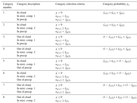
Table 1. For each of the eight categories, this table lists (1) the category number; (2) whether the category is cloudy, in mixture component

1 or 2, or precipitating; (3) what inequalities must be satisfied for a sample point to lie within the category; and (4) the original probability

mass associated with the category,pj.

Category Category description Category selection criteria Category probabilitypj

number

1 In cloud

In mixt. comp. 1 In precip

χ >0

ud+1< ξ(1)

ud+2< fp(1)

fc(1)×ξ(1)×fp(1)

2 In cloud

In mixt. comp. 2 In precip

χ >0

u_d+1≥ξ(1)

ud+2< fp(2)

fc(2)×ξ(2)×fp(2)

3 Out of cloud

In mixt. comp. 1 In precip

χ≤0

ud+1< ξ(1)

ud+2< fp(1)

(1−fc(1))×ξ(1)×fp(1)

4 Out of cloud

In mixt. comp. 2 In precip

χ≤0

ud+1≥ξ(1)

u_d+2< fp(2)

(1−fc(2))×ξ(2)×fp(2)

5 In cloud

In mixt. comp. 1 Out of precip

χ >0

ud+1< ξ(1)

ud+2≥fp(1)

fc(1)×ξ(1)×(1−fp(1))

6 In cloud

In mixt. comp. 2 Out of precip

χ >0

ud+1≥ξ(1)

ud+2≥fp(2)

fc(2)×ξ(2)×(1−fp(2))

7 Out of cloud

In mixt. comp. 1 Out of precip

χ≤0

u_d+1< ξ(1)

ud+2≥fp(1)

(1−fc(1))×ξ(1)×(1−fp(1))

8 Out of cloud

In mixt. comp. 2 Out of precip

χ≤0

ud+1≥ξ(1)

ud+2≥fp(2)

(1−fc(2))×ξ(2)×(1−fp(2))

a mathematical form for the new PDF that points are drawn from, we introduce some notation. We define a new function, L(x), called the “likelihood ratio”:

L(x)≡

Ncat

X

j=1

_p

j

Sj

·1j(x)≡ Ncat

X

j=1

ωj1j(x). (9)

Here, 1j(x)is the indicator function of categoryCj, defined

as 1j(x)=

(

1 x∈Cj

0 x6∈Cj

, (10)

and ωj=

pj

Sj

(11) is the weight of each sample point in categoryCj. Then, the

new sampling PDF, denotedQ(x), is defined as Q(x)=P (x)

L(x). (12)

The new PDF, Q(x), is normalized because PNcat

j=1Sj=1.

The integral in Eq. (2) is written as

Z

h(x)P (x)dx=

Z

h(x)L(x) _{P (x)}

L(x)

dx =

Z

h(x)L(x)Q(x)dx. (13)

Then, the new integral in Eq. (13) is approximated by draw-ingNs sample points from theQ(x)distribution and

evalu-ating

Z

h(x)L(x)Q(x)dx≈ 1 Ns

Ns

X

i=1

h(xi)L(xi), (14)

wherexi is theisample point drawn from theQ(x)

distribu-tion. For a sample pointxiin categoryCj,L(xi)=p_Sj

j =ωj.

To draw sample points from theQ(x)distribution, a uni-form variate, 0< uc<1, is picked for each sample point.

will be associated with categoryC1. IfS1≤uc< S1+S2, the

sample will be associated with categoryC2, and so on. Once

the category has been determined, the sample point is drawn from the portion of the marginal distribution ofP (x)that is within the category. For example, a sample point that is to be in cloud is drawn from the distributionP (x|χ >0). 4.1 The weight limiter

Importance sampling allows the modeler to concentrate sam-ple points in areas of the samsam-ple space that are considered important. But sample points given to important areas are taken from unimportant areas. Therefore, if importance sam-pling is applied overzealously, the less important processes can become excessively noisy.

In SILHS, we wish to employ an importance sampling scheme that improves results for important processes (e.g., certain microphysical processes) while still producing rea-sonably accurate estimates of other “less important” or per-haps less variable processes. One reason that we wish to avoid overdoing the importance sampling is that a favorable sampling distribution at one grid level (altitude) may be un-favorable at another.

The change in accuracy for a given category due to im-portance sampling can be assessed by noting the weight of sample points in that category. The inverse weight of a sam-ple point in categoryCjis given by

1 ωj

=Sj pj

, (15)

wherepj is the category’s original probability andSj is the

category’s modified probability due to importance sampling. The weight,ωj, is closely related toL(x)(see Eq. 9). The

inverse weight, 1/ωj, may be interpreted as the density of

sample points per unit probability mass. When 1/ωj<1, the

category is sampled less often with importance sampling, and when 1/ωj>1, the category is sampled more often with

im-portance sampling. We are particularly concerned about large values ofωj, because large weights are associated with

un-dersampling and hence degradations in accuracy.

In order to mitigate the negative impact of importance sampling, we now propose a simple method to impose a max-imum weight,ωmax, in each category. Intuitively, the

algo-rithm works as follows. For each category Cj, we compute

the minimum modified sampling probability: Sj,min=

pj ωmax

. (16)

To ensure that the weight of a category, ωj, does not

ex-ceed ωmax, the category must be sampled at least as often

as Sj,min; that is, Sj≥Sj,min. If any categories are

under-sampled, thenSj must be increased in those categories, and

probability mass must be taken from other categories (where Sj > Sj,min) in order to ensure that theSj probabilities sum

to 1. The algorithm takes probability mass from another cate-gory in proportion to how much “extra” probability mass the category has.

Formally, the algorithm is constructed as follows. We com-pute the difference between the category’s modified probabil-ity,Sj, and its minimum modified probability,Sj,min:

Sj,diff=Sj−Sj,min. (17)

LetNbe the set of all categories whereSj,diff<0 (the

cate-gories whereSj needs to be increased) andMbe the set of

all categories whereSj,diff≥0 (the categories whereSj can

potentially be reduced). IfN is the empty set (that is, if no categories haveSdiff<0), then all categories already satisfy

the weight limit, and nothing needs to be done. Otherwise, if S_j0 is the new distribution of modified probabilities, then for allCj∈Nwe set

S_j0 =Sj,min, (18)

and for allCj∈Mwe set

S_j0 =Sj− 

 Sj,diff·



 

P

Ci∈N

Si,diff

P

Ci∈M

Si,diff 

  



. (19)

This method will take sampling probability away from the categories with extra probability proportionally to how much extra probability they have (i.e., how largeSj,diff is). It can

readily be shown that the fractionsS_j0 are bound to the range [0,1]and sum to 1.

In SILHS, we currently setωmax=2, which means that on

average, a category will be sampled no less than half as of-ten with importance sampling than without importance sam-pling. Consequently, the variance of the estimate of a quan-tity is increased (degraded) by no more than a factor of 2 due to importance sampling. (The standard deviation is in-creased by no more than a factor of

√

2≈1.4. For this esti-mate of variance, we assume the usual Monte Carlo conver-gence rate.)

4.2 Optimal allocation of sample points

The success of the nCat method depends on knowing how to allocate sample points to the categories. In some cases, it is easy to see how to allocate points. For example, if it is known that the process(es) of interest are active in only one of the Ncatcategories, then we can simply put all sample points in

that one category, and use the weight limiter to ensure that other categories are still adequately sampled. However, in the case that processes of interest are active in two or more cate-gories, one needs to know how to distribute (i.e., “allocate”) sample points among these categories.

sample points (Lemieux, 2009). The optimal allocation pro-vides guidance on how to determine the Sj values. In

Ap-pendix A, it is shown that the optimal modified probabilities are

Sj = pj

√ vj PNcat

i=1pi

√ vi

. (20)

This expression shows that the optimal fraction of samples in categoryCj, i.e.,Sj, depends on both the original probability pj of category Cj, and on the category-averaged standard

deviation,√vj.

4.3 A simple method of allocating sample points One could prescribe the modified probabilities Sj directly.

However, a key problem with directly prescribing theSj is

that prescribed values cannot scale with the original prob-abilities pj. For instance, consider the case in which, for

some category Cj, we have prescribed Sj>0, but it turns

out that for a particular cloud case,pj=0. Then some

sam-ple points will be placed in category Cj even though they

contribute nothing to the overall sum. (These sample points have a weight of zero.) This is a needless computational ex-pense. Instead, the sample points should be placed in other categories with non-zeropj.

More generally, prescribing eachSj directly is akin to

as-suming that the contribution of each category to the total sum is constant regardless of what fraction of the PDF is occupied by each category. Instead, a more realistic assumption is that each category contributes to the total sum a constant amount

per unit original probability,pj. These prescribed amounts

are then scaled by the original probabilitiespj to obtain the

modified probabilitiesSj.

Specifically, we prescribe the following normalized stan-dard deviation of the process rate for each categoryCj: γj=

√ vj PNcat

i=1

√ vi

. (21)

To make theγjeasier to interpret and prescribe, we insist that

0≤γj ≤1; then the denominator is simply the sum of the

numerator in all categories, so that eachγj is a fraction with PNcat

j=1γj=1. Specifically,γj is the fraction of

√

vj in

cat-egoryCj. Prescribingγj is accurate and general when each γj varies little in space or time, or from case to case. Note

that the numerator of Eq. (21) is the same as the numerator of Eq. (20), but without thepj term.

Given theγjfractions, it is easy to determine theSjvalues

by dividing the numerator and denominator of Eq. (20) by

PNcat

i=1

√

vi. This yields Sj =

pjγj PNcat

i=1piγi

. (22)

It is clear from this equation that theSj values are still in the

range[0,1]and still sum to 1.

The prescription (Eq. 22) leads to more robust impor-tance sampling than does prescribingSj values as constants.

With Eq. (22), the optimalγj in a particular category (say,

in cloud and precipitation and mixture component 1) is rela-tively insensitive to the area occupied by that category (e.g., to the cloud fraction or precipitation fraction). The reason is that in Eq. (22), eachSj value weights γj by the original

probabilitypj of categoryCj. This means that, for instance,

whenCj occupies a small fraction of the domain, andγj is

moderate, then the total fraction of sample pointsSj in

cat-egoryCj scales naturally to small values. Prescribing theγj

values is akin to prescribing the inverse weights 1/ωj, rather

than the sample fractionsSj. To see resemblance ofγj and

1/ωj, note from Eqs. (15) and (22) that

1 ωj

= Sj pj

= γj

PNcat

i=1piγi

. (23)

Both 1/ωj andγjare related to the density of sample points

per unit probability mass,pj.

4.4 Advantages of the new method

As compared to the previous version of SILHS, the chief ad-vantage of the new nCat method is its flexibility. In particu-lar, the user can individually prescribe the sampling density per unit probability (γj) in each of eight categories,Cj. This

flexibility is useful when important processes, such as evap-oration of rain, occur in particular categories, such as the re-gion of rain but no cloud.

This flexibility is made possible in part by the fact that the nCat method imposes no restriction on the number of sam-ple points used per timestep. The previous version of SILHS required an even number of sample points per timestep, be-cause one point was placed in cloud and the other was placed outside cloud. Generalizing this method to eight categories would have required a multiple of at least eight sample points per timestep, and would not allow much flexibility in pre-scribing the relative importance of categories. Instead, the nCat method uses a probabilistic approach to picking a cate-gory for each sample point. This allows any number of sam-ple points to be used at each timestep, including the use of fewer thanNcatsamples, without causing a biased result.

4.5 Summary of steps to implement method

In summary, to implement the new importance sampling method, the following steps should be taken.

1. Pick a set of categories,Cj, that span the PDF domain.

We have proposed eight categories for use, as given in Table 1.

2. Pick a set of sampling fractions,γj. A good set of

3. Compute, from the fractionsγj, the modified

probabili-tiesSjusing Eq. (22). Pick sample points from theQ(x)

distribution, defined in Eq. (12).

4. Compute the weight in each category, ωj, using

Eq. (11). Sample points are given a weight correspond-ing to the category the sample point is in. Limit the weights according to the algorithm in Sect. 4.1, if so desired.

5. Feed the (unweighted) sample points one by one into a physical parameterization (e.g., a microphysics scheme).

6. Compute a weighted average of the function of interest using Eq. (14).

5 Methodology of evaluation of the sampling methods In order to evaluate how well the new importance sampling scheme simulates multiple cloud types, we have simulated two cloud cases. The first is a drizzling shallow cumulus case: Rain in shallow Cumulus over the Ocean (RICO), con-figured as in the intercomparison of vanZanten et al. (2011). RICO was a drizzling trade-wind cumulus case observed off the Caribbean islands of Antigua and Barbuda (Rauber et al., 2007). The second is a drizzling stratocumulus case: Research Flight 2 (RF02) of the DYnamics and Chemistry Of Marine Stratocumulus (DYCOMS-II), configured as in Wyant et al. (2007). DYCOMS-II RF02 was a nocturnal drizzling stratocumulus layer observed off the coast of Cal-ifornia (Stevens et al., 2003). A key difference in the sam-pling of these two cases is that the stratocumulus case has a much larger cloud fraction (>0.95) than the cumulus case (<0.05). Therefore, without importance sampling, nearly all sample points fall in cloud in the stratocumulus case, while almost none fall in cloud in the cumulus case. Finding a sin-gle, effective sampling strategy for both the stratocumulus and cumulus cases is challenging.

The following four configurations of SILHS were used for comparison.

1. “LH-only”. This configuration uses only Latin hyper-cube sampling. No importance sampling is performed. The nCat method is not used.

2. “2Cat-Cld”. This configuration is functionally equiva-lent to the old version of SILHS that placed one point in cloud and one point out of cloud. This configura-tion uses two categories: in cloud, and out of cloud. The categories (c,p,1), (c,p,2), (c,np,1), and (c,np,2) are all lumped together into the “cloud” category, and the other four categories are analogously lumped into the “clear” category. That is, a point that is in cloud belongs to the cloud category regardless of whether it is in precipita-tion or which mixture component it is in, and similarly

for points in clear air. When cloud fraction is between 0.5 and 50 %, it places 50 % of sample points in each of the two categories. (That is,S1=S2=0.5.) Otherwise,

no importance sampling is performed.

3. “2Cat-CldPcp”. This configuration also uses two cat-egories. The first consists of points that are either in cloud or in precipitation, and the second consists of the complement, namely, points that are neither in cloud nor in precipitation. That is, (nc,np,1) and (nc,np,2) are lumped into the no-cloud-or-precipitation category, and the others are lumped into the cloud-or-precipitation category. Since no microphysical processes act in the area of the domain outside of cloud and precipita-tion, the sample points are initially prescribed such that all points fall in the cloud-or-precipitation cate-gory (i.e., the first catecate-gory). (That is,γ1=S1=1, γ2= S2=0). After the initial prescription, the weight limiter

ensures thatS2=_ωp_max2 =p₂2.

4. “8Cat”. This configuration uses all eight categories listed in Table 1. To determine the sampling fractionsγj

to use, a simulation was run in which SILHS was used to estimate the quantity in Eq. (21) at each timestep. One set of sampling fractions,γj, was used for both RICO

and DYCOMS-II RF02. This is discussed in Sect. 6.1. The simulations were non-interactive, so that errors in the SILHS simulations did not feed back into the simulated fields. This made it possible to evaluate multiple SILHS sim-ulations against a common analytic solution. Some notable aspects of the simulation configurations are shown in Table 2. The microphysics scheme used in the simulations is that of Khairoutdinov and Kogan (2000). As a reference solu-tion, an analytically upscaled version of the Khairoutdinov– Kogan microphysics scheme was used, as described in Lar-son and Griffin (2013). CompariLar-son with the analytic so-lution indicates whether SILHS draws sample points from the correct PDF at each grid level. However, the comparison with the analytic solution does not test whether the PDFs at each level are overlapped accurately. Although the overlap assumptions do not affect these test cases, overlap does in-fluence processes such as radiative transfer. Testing the PDF overlap assumptions is left for future research. Nevertheless, the ability to test convergence at each grid level is an advan-tage. For instance, early convergence tests revealed several bugs in SILHS. Many microphysics schemes in operational use do not permit analytic solution. For these microphysics schemes, a non-analytic integration method, such as SILHS, is necessary.

Each SILHS configuration was evaluated on its ability to estimate the following three microphysical processes.

Table 2. Notable configuration settings for the RICO and DYCOMS-II RF02 simulations performed in this paper.

RICO DYCOMS-II RF02

Timestep (s) 300 60

Vertical levels 128 160

Vertical grid spacing (m) 25–250 10

Radiation None Analytic longwave (Larson et al., 2007)

Cloud droplet concentration (m−3) 70×106 55×106

2. Accretion: the growth of rain droplets by collection of cloud water. This process occurs when both cloud and precipitation are present.

3. Evaporation: the conversion of rain water to water va-por. This process occurs in areas outside cloud but within precipitation.

6 Simulations of drizzling cumulus and stratocumulus clouds

In this section, we present results obtained using the new im-portance sampling method.

6.1 Estimation of optimal sampling fractions

Prescribing the γj is a useful general approach only if the γj vary relatively little from case to case. We test this by

estimating the optimal sampling fractions, γj, for both the

RICO and DYCOMS-II RF02 cases. The optimalγj values

are calculated by estimating the right-hand side of Eq. (21) at each timestep at the importance sampling level. The process used,h(x), is the sum of the autoconversion, accretion, and evaporation tendencies from the microphysics scheme. The importance sampling level is chosen at each timestep to be the level with the maximum within-cloud cloud water mass mixing ratio. The integral definingvj, given in Eq. (A4), was

estimated using 256 SILHS sample points. The γj values,

averaged over all timesteps (864 total timesteps for RICO and 360 for DYCOMS-II RF02), are shown in Table 3.

We see that in both cases, the optimalγjvalues are largest

in category 1 (in cloud, in precipitation, and in mixture com-ponent 1) and in category 3 (out of cloud, in precipitation, and in mixture component 1). As expected, the optimal sam-pling fractions for the last two categories are zero, since mi-crophysical processes do not act in the region where neither cloud nor rain exists. The other categories show differences, which may or may not be important. To test this, the optimal fractions for DYCOMS-II RF02 shown in Table 3 are used for both RICO and DYCOMS-II RF02 simulations to be pre-sented. Thereby, the RICO case is used to test the robustness of the DYCOMS-II RF02 sampling fractions.

100 ₁₀1 ₁₀2 ₁₀3

10-11

10-10

10-9

10-8

RM

SE

of

S

ILH

S

es

tim

at

e

[k

g

kg

−

1s

−

1]

Autoconversion ³_r

r

t

´ auto

100 ₁₀1 ₁₀2 ₁₀3

10-9

10-8

10-7 Accretion

³_r

r

t

´ accr

100 ₁₀1 ₁₀2 ₁₀3

Number of sample points 10-10

10-9

10-8

10-7

RM

SE

of

S

ILH

S

es

tim

at

e

[k

g

kg

−

1s

−

1]

Evaporation ³_rr

t

´ evap

100 ₁₀1 ₁₀2 ₁₀3

Number of sample points 10-9

10-8

10-7 Auto + Accr + Evap

LH-only

2Cat-Cld 2Cat-CldPcp8Cat

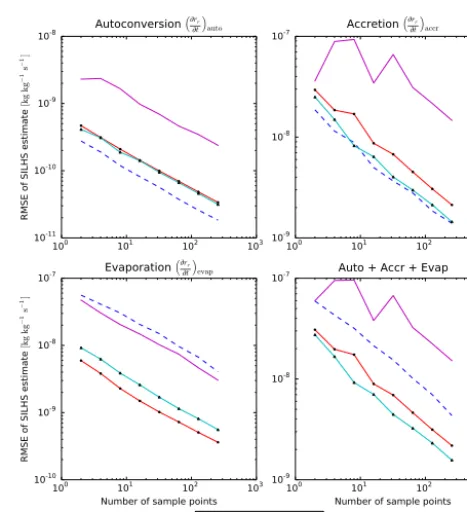
Figure 1. RICO: the root-mean-square error (RMSE) at the

im-portance sampling level of SILHS simulations as a function of the number of sample points, for the RICO cumulus case. The error is time-averaged over the entire simulation. The 2Cat-CldPcp and 8Cat methods show a large improvement over the 2Cat-Cld and LH-only methods in the estimate of evaporation, but not for autoconve-sion and accretion, which are in-cloud processes. Nevertheless, the 8Cat and 2Cat-CldPcp methods both impove the estimate of the sum of the three processes.

6.2 Results for RICO case

Figure 1 shows a plot of the root-mean-square error (RMSE) of the SILHS RICO simulations as a function of the num-ber of sample points used. The 8Cat method has the smallest RMSE of all three methods when estimating the sum of au-toconversion, accretion, and evaporation.

Table 3. Estimated optimal sampling fractions (γ_j) for each importance category, averaged over the entire simulation, for the RICO and DYCOMS-II RF02 cases. These estimates were obtained by using SILHS to estimate the right-hand side of Eq. (21) for each category. Here “c” denotes “in-cloud”, “nc” denotes “out of cloud”, “p” denotes “in-precipitation”, “np” denotes “out of precipitation”, “1” denotes “in mixture component 1”, and “2” denotes “in mixture component 2”.

Category 1 2 3 4 5 6 7 8

(c,p,1) (c,p,2) (nc,p,1) (nc,p,2) (c,np,1) (c,np,2) (nc,np,1) (nc,np,2)

RICO 0.539 0.004 0.223 0.203 0.033 0.004 0.000 0.000

DYCOMS-II RF02 0.351 0.143 0.238 0.061 0.140 0.070 0.000 0.000

Table 4. RICO: percentage of sample points allocated to each

cat-egory by each sampling method at the importance sampling level, time-averaged over the entire simulation. The more sample points placed in a particular category, the better the estimate of processes active in that category.

Category 8Cat 2Cat-CldPcp 2Cat-Cld LH-only

(c,p,1) 12.1 5.7 13.6 0.3

(c,p,2) 0.03 0.03 0.04 0.02

(nc,p,1) 16.1 11.0 0.3 0.5

(nc,p,2) 7.9 18.8 0.4 0.7

(c,np,1) 14.8 15.4 36.0 0.7

(c,np,2) 0.2 0.3 0.4 0.2

(nc,np,1) 0.7 0.7 0.7 1.3

(nc,np,2) 48.2 48.2 48.7 96.3

poorly sampled in the 2Cat-Cld method is that the 2Cat-Cld method performs importance sampling only within cloud. In-deed, for in-cloud processes, such as autoconversion and ac-cretion, the 2Cat-Cld method equals or improves upon both the 2Cat-CldPcp method and the 8Cat method in the RICO cumulus case. However, the 2Cat-Cld method reduces the number of sample points outside of cloud, degrading the sim-ulation of rain evaporation. In contrast, both the 2Cat-CldPcp and 8Cat methods preferentially sample within the region of the sample space containing evaporation (out of cloud but within precipitation), leading to large improvements.

Table 4 compares how each of the four sampling meth-ods allocates sample points. The table shows the percentage of sample points allocated to each category, averaged over the simulation. Comparing the allocation between the meth-ods can give insight into the strengths and weaknesses of each method. For example, evaporation is best sampled by the 8Cat and 2Cat-CldPcp methods because they are the only methods that place a sizable number of points in the two cat-egories that are in precipitation and outside cloud. The 2Cat-Cld and 8Cat methods give the best estimate of accretion be-cause they place the largest number of points in the categories that are within cloud and precipitation.

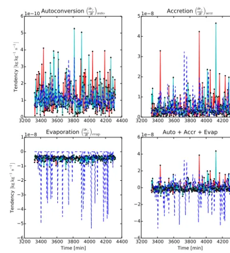
Figure 2 shows, for the RICO case, time-series plots of the four tendencies at the importance sampling level. Again, the largest improvement can be seen in the sampling of evapo-ration. Looking at the 2Cat-Cld time series for evaporation,

3200 3400 3600 3800 4000 4200 44000

1 2 3 4 5 6

Te

nd

en

cy

[k

g

kg

−

1s

−

1]

1e 10Autoconversion ³rr

t

´

auto

3200 3400 3600 3800 4000 4200 44000

1 2 3 4

51e 8 Accretion

³_rr

t

´

accr

3200 3400 3600 3800 4000 4200 4400 Time [min]

6 5 4 3 2 1 0 1

Te

nd

en

cy

[k

g

kg

−

1s

−

1]

1e 8 Evaporation ³rr

t

´

evap

3200 3400 3600 3800 4000 4200 4400 Time [min]

6 4 2 0 2 4

6 1e 8 Auto + Accr + Evap

2Cat-CldPcp

8Cat 2Cat-Cld

Figure 2. RICO: time-series plots of the four tendencies at the

im-portance sampling level. The simulations in these plots use 32 sam-ple points, and the plots show minutes 3321 to 4320 of the simu-lations. To improve readability, the LH-only method is not plotted. The evaporation tendencies are much more noisy in the 2Cat-Cld method than in the 2Cat-CldPcp or 8Cat methods.

it can be seen that at many timesteps, no points are found in the evaporating region of the sample space (out of cloud and within precipitation), and the estimated evaporation tendency is zero. At the timesteps where one or more sample points are found in the evaporating region, the tendency estimate is very large because the evaporation rate within the evaporating re-gion is much larger than the overall mean evaporation rate. In the 2Cat-CldPcp and 8Cat simulations, the evaporating re-gion of the sample space is well sampled, and sample points in this region have small weights, leading to an estimate that is much more comparable to the overall mean.

0.0 0.2 0.4 0.6 0.8 1.0 1.2 1.4 1e 10 0

500 1000 1500 2000 2500 3000 3500 4000

Height [m]

Autoconversion ³_rr

t

´ auto

0.0 0.2 0.4 0.6 0.8 1.0 1.2 1.4 1.6 1e 8 0

500 1000 1500 2000 2500 3000 3500

4000 Accretion

³_rr

t

´ accr

1.2 1.0 0.8 0.6 0.4 0.2 0.0 Tendency [kg kg−1_s−1_] 1e 8 0

500 1000 1500 2000 2500 3000 3500 4000

Height [m]

Evaporation ³_rr

t

´ evap

1.5 1.0 0.5 0.0 0.5 1.0 1.5 Tendency [kg kg−1_s−1_] 1e 8 0

500 1000 1500 2000 2500 3000 3500

4000 Auto + Accr + Evap

2Cat-CldPcp

8Cat 2Cat-CldAnalytic

Figure 3. RICO: mean profile plots of the four tendencies. The

sim-ulations in these plots use 32 sample points. For each configuration, an ensemble of 12 simulations is used, each with a different seed. Profiles are averaged over all 864 timesteps of the simulation and all 12 ensemble members. It is seen that all SILHS sampling methods are clearly convergent at all height levels.

(over height levels) were generated for simulations with 32 sample points. To reduce the role of a “lucky” random seed in the comparison and thereby better distinguish the meth-ods, an ensemble of 12 simulations was used. Figure 3 shows profile plots of the four tendencies over height levels. These plots are averaged over all 864 timesteps and over the 12 en-semble members, and serve to indicate that SILHS converges to the analytic solution at all height levels and not only the importance sampling level. Figure 4 shows the RMSE of the SILHS solutions at each height level compared to the analytic solution, for all timesteps and ensemble members. It can be seen that the 8Cat and 2Cat-CldPcp methods show improved results compared to the 2Cat-Cld method at height levels be-tween 1000 and 2500 m. These height levels are where the improvement in the evaporation term is strongest. At levels below 1000 m (which are far below the importance sampling level of about 2000 m), all methods start to show consider-able noise. It is interesting that this noise remains even after time and ensemble averaging. This highlights the large de-gree of variability in cumulus clouds and the need for careful parameterization of this variability.

We note that, in this paper, only the profile plots display an ensemble average. The time-series plots display a single simulation so that individual sample values can be seen. The

0.0 0.5 1.0 1.5 2.0 2.5 3.0 1e 10 0

500 1000 1500 2000 2500 3000 3500 4000

Height [m]

Autoconversion ³_rr

t

´ auto

0 1 2 3 4 5 6 7 8 1e 8 0

500 1000 1500 2000 2500 3000 3500

4000 Accretion

³_rr

t

´ accr

0.0 0.5 1.0 1.5 2.0 RMSE of tendency [kg kg−1s ]−1 1e 8 0

500 1000 1500 2000 2500 3000 3500 4000

Height [m]

Evaporation ³_rr

t

´ evap

0 1 2 3 4 5 6 7 8 RMSE of tendency [kg kg−1s ]−1 1e 8 0

500 1000 1500 2000 2500 3000 3500

4000 Auto + Accr + Evap

2Cat-CldPcp

8Cat 2Cat-Cld

Figure 4. RICO: profile RMSE plots of the four tendencies. The

simulations in these plots use 32 sample points. For each configu-ration, an ensemble of 12 simulations is used, each with a different seed. RMSE values are averaged over all 864 timesteps of the sim-ulation and all 12 ensemble members. The 8Cat and 2Cat-CldPcp methods show improvement between 1000 m and 2500 m, where the improvement in sampling of the evaporation term is largest. All three methods suffer from extra noise below 1000 m, which is far away from the importance sampling level. The importance sampling level is just under 2000 m for most timesteps in the simulation.

plots displaying RMSE vs. the number of sample points are not strongly influenced by the choice of random seed. 6.3 Results for DYCOMS-II RF02 case

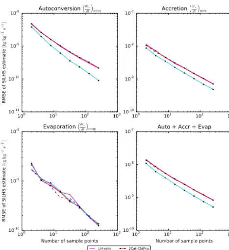
The other simulated case is DYCOMS-II RF02, a drizzling stratocumulus case. Figure 5 shows a plot of the RMSE of the SILHS simulations as a function of the number of sample points. The LH-only, 2Cat-Cld, and 2Cat-CldPcp simulations all show approximately the same amount of noise. However, the 8Cat method reduces noise in autoconversion and accre-tion, thereby also decreasing noise in the sum of the three tendencies.

100 ₁₀1 ₁₀2 ₁₀3 10-11 10-10 10-9 10-8 RM SE of S ILH S es tim at e [k g kg − 1s − 1]

Autoconversion ³_rr

t

´ auto

100 ₁₀1 ₁₀2 ₁₀3

10-10

10-9

10-8

10-7 Accretion

³_rr

t

´ accr

100 ₁₀1 ₁₀2 ₁₀3

Number of sample points 10-10 10-9 10-8 RM SE of S ILH S es tim at e [k g kg − 1s − 1]

Evaporation ³_rr

t

´ evap

100 ₁₀1 ₁₀2 ₁₀3

Number of sample points 10-10

10-9

10-8

10-7 Auto + Accr + Evap

LH-only

2Cat-Cld 2Cat-CldPcp8Cat

Figure 5. DYCOMS-II RF02: the root-mean-square error (RMSE)

of SILHS simulations as a function of sample points for the DYCOMS-II RF02 stratocumulus case. The error is calculated at the importance sampling level and is averaged over all timesteps of the simulation. The LH-only, 2Cat-Cld, and 2Cat-CldPcp meth-ods are expected to have roughly the same behavior in a case like DYCOMS-II RF02 that has cloud fraction near 100 %. The 8Cat method still improves the estimates of autoconversion and accre-tion because it is able to flexibly allocate points within the cloudy region of the sample space.

Table 5. DYCOMS-II RF02. Percentage of sample points allocated

to each category by each sampling method at the importance sam-pling level, time-averaged over the entire simulation. The more sample points placed in a particular category, the better the estimate of processes active in that category.

Category 8Cat 2Cat-CldPcp 2Cat-Cld LH-only

(c,p,1) 57.3 35.0 35.1 35.1

(c,p,2) 41.2 63.0 63.0 63.1

(nc,p,1) 0.5 0.5 0.5 0.5

(nc,p,2) 0.2 0.3 0.3 0.3

(c,np,1) 0.6 0.7 0.7 0.7

(c,np,2) 0.2 0.4 0.4 0.4

(nc,np,1) 0 0 0.01 0.02

(nc,np,2) 0.03 0.04 0.07 0.07

points in the second category (the category without cloud or precipitation) by only a factor of 2. Since the second cate-gory is so small to begin with (that is,p2is very small), this

reduction hardly improves the result at all.

150 200 250 300 350 400

0.7 0.8 0.9 1.0 1.1 1.2 1.3 Te nd en cy [k g kg − 1s − 1]

1e 8 Autoconversion ³rr

t

´

auto

150 200 250 300 350 400

0.5 1.0 1.5 2.0 2.5 3.0

3.51e 8 Accretion

³_rr

t

´

accr

150 200 250 300 350 400

Time [min] 5 4 3 2 1 0 Te nd en cy [k g kg − 1s − 1]

1e 9 Evaporation ³rr

t

´

evap

150 200 250 300 350 400

Time [min] 1.0 1.5 2.0 2.5 3.0 3.5 4.0

4.5 1e 8 Auto + Accr + Evap

2Cat-CldPcp

8Cat 2Cat-Cld

Figure 6. DYCOMS-II RF02: time-series plots of the four

tenden-cies at the importance sampling level. The simulations in these plots use 32 sample points. The time range plotted includes minutes 161 to 360 of the simulation. The evaporation process is poorly sampled in all three sampling methods, but it is a relatively small term and makes a much smaller contribution to the sum of the three processes than autoconversion and accretion.

The reason for the improvement using the 8Cat method can be inferred from Table 5. The table shows the percent-age of sample points allocated to each category at the im-portance sampling level, averaged over the entire simulation. The 2Cat-CldPcp, 2Cat-Cld, and LH-only allocations are all similar, but the 8Cat allocation places more points in (c,p,1) than (c,p,2). That is, unlike the other three methods, the 8Cat method is able to preferentially sample from mixture com-ponent 1. Comcom-ponent 1, in turn, contains larger cloud (liq-uid) water mixing ratios. The other three methods necessar-ily place more points in component 2 than component 1, because component 2 occupies more of the (original) PDF. However, it was shown in Table 3 that optimally, component 1 has a much higher per-probability sampling density than does component 2. This increased sampling of component 1 is the source of the improvement of the 8Cat method.

Table 6. Number of sample points needed by each configuration

of SILHS to achieve a given RMSE in estimating the sum of the three processes, for the RICO and DYCOMS-II RF02 cases. These numbers are estimated visually from Figs. 1 and 5. In RICO, the 2Cat-CldPcp method requires approximately a factor of 4 fewer sample points than the 2Cat-Cld method to achieve an RMSE of

10−8kg kg−1, and 8Cat method requires approximately a factor of

8 fewer sample points. In DYCOMS-II RF02, the 8Cat method re-quires approximately a factor of 1.6 fewer sample points than the 2Cat-CldPcp, 2Cat-Cld, and LH-only methods to achieve an RMSE

of 4×10−9kg kg−1.

Method Samples for Samples for 4×10−9

10−8RMSE (RICO) RMSE (DYCOMS-II RF02)

LH-only ∼700 13

2Cat-Cld 65 13

2Cat-CldPcp 15 13

8Cat 8 8

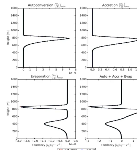
Figure 7 shows the mean profile plots of the four tenden-cies. Once again, an ensemble of 12 simulations was used, and each sampling method overplotted is averaged over all timesteps and 12 ensemble members. All of the lines look similar, which indicates that all three methods do a good job of sampling the three processes with 32 sample points per timestep, perhaps because the DYCOMS-II RF02 stra-tocumulus case is not highly variable. Figure 8 shows profile RMSE plots averaged over all timesteps and ensemble mem-bers. All sampling methods show the largest RMSE at around 800 m. At this level, the 8Cat method shows smaller error in autoconversion and accretion, but all methods show about the same error in evaporation.

Table 6 shows a quantitative comparison of the four con-figurations for both the RICO and DYCOMS-II RF02 cases. For each sampling method, Table 6 lists the approximate number of sample points needed to obtain the given time-averaged RMSE at the importance sampling level. These val-ues are estimated visually from Figs. 1 and 5. This table shows that in RICO, the 8Cat method requires approximately a factor of 8 fewer points to achieve a desired RMSE than the 2Cat-Cld method. The 2Cat-CldPcp method requires approx-imately a factor of 4 fewer sample points than the 2Cat-Cld method. In DYCOMS-II RF02, the reduction of necessary sample points for the given RMSE for the 8Cat method as compared to the others is a factor of approximately 1.6. 6.4 Computational cost of the nCat method

An important consideration among Monte Carlo integration methods is their computational cost. The cost of the new nCat method was tested against both the prior SILHS importance sampling method and the cost of CLUBB. Eight SILHS sam-ple points were used in each simulation. Five RICO simu-lations were performed, and Table 7 shows the means and standard deviations of the five simulations. Each time is a

0 1 2 3 4 5 6 7 8 1e 9 0

200 400 600 800 1000 1200 1400 1600

Height [m]

Autoconversion ³_r

r

t

´ auto

0.0 0.2 0.4 0.6 0.8 1.0 1.2 1.4 1e 8 0

200 400 600 800 1000 1200 1400

1600 Accretion

³_r

r

t

´ accr

3.0 2.5 2.0 1.5 1.0 0.5 0.0 0.5 Tendency [kg kg−1_s−1_] 1e 8 0

200 400 600 800 1000 1200 1400 1600

Height [m]

Evaporation ³_r

r

t

´ evap

3 2 1 0 1 2

Tendency [kg kg−1_s−1_] 1e 8 0

200 400 600 800 1000 1200 1400

1600 Auto + Accr + Evap

2Cat-CldPcp

8Cat 2Cat-CldAnalytic

Figure 7. DYCOMS-II RF02: mean profile plots of the four

ten-dencies. The simulations in these plots use 32 sample points. For each configuration, an ensemble of 12 simulations is used, each with a different seed. Profiles are averaged over all 360 timesteps of the simulation and all 12 ensemble members. It is seen that all SILHS sampling methods are clearly convergent at all height levels. All of the lines overlap well, indicating that all three processes are sampled well by all three sampling methods.

cumulative total of the respective component of the model over the entire simulation. The two nCat methods (2Cat-CldPcp and 8Cat) show no significant increase in compu-tation time as compared to the original SILHS importance sampling method. All SILHS methods are about twice as ex-pensive as CLUBB when eight sample points are used.

These costs may be compared with other costs in global climate simulations. To this end, Thayer-Calder et al. (2015) tested the cost of SILHS in the Community Atmosphere Model (Neale et al., 2012). They show that an adequate cloud climatology can be obtained with as few as four sam-ple points (see Figs. 12 and 13 of Thayer-Calder et al., 2015). The extra cost of computing four samples is (1.89– 1.69)/1.69=16 % (see Table 2 of Thayer-Calder et al., 2015).

7 Conclusions

We have developed a new (“nCat”) method to sample sub-grid variability in atmospheric models. The method divides the grid box sample space intoNcatcategories and allows the

0 1 2 3 4 5 6 7 8 1e 10 0

200 400 600 800 1000 1200 1400 1600

Height [m]

Autoconversion ³_r

r

t

´ auto

0.0 0.5 1.0 1.5 2.0 2.5 1e 9 0

200 400 600 800 1000 1200 1400

1600 Accretion

³_r

r

t

´ accr

0.0 0.5 1.0 1.5 2.0 2.5 RMSE of tendency [kg kg−1s ]−1 1e 8 0

200 400 600 800 1000 1200 1400 1600

Height [m]

Evaporation ³_r

r

t

´ evap

0.0 0.5 1.0 1.5 2.0 2.5 RMSE of tendency [kg kg−1s ]−1 1e 8 0

200 400 600 800 1000 1200 1400

1600 Auto + Accr + Evap

2Cat-CldPcp

8Cat 2Cat-Cld

Figure 8. DYCOMS-II RF02: profile RMSE plots of the four

ten-dencies. The simulations in these plots use 32 sample points. For each configuration, an ensemble of 12 simulations is used, each with a different seed. RMSE values are averaged over all 360 timesteps of the simulation and all 12 ensemble members. All sampling meth-ods show the largest RMSE at around 800 m. At this level, the 8Cat method shows smaller error in autoconversion and accretion, but all methods show about the same error in evaporation.

The most flexible variant of the nCat method that we consider here breaks the grid box into eight categories, de-pending on whether a parcel contains cloud droplets or rain droplets, or is within the first mixture component of the PDF. This “8Cat” variant allows a fine degree of control over where the samples are placed.

Another variant has been created by lumping the eight sep-arate categories into two: one that contains either cloud or precipitation, and one that contains neither cloud nor precip-itation. This (“2Cat-CldPcp”) variant is useful when the user does not have an estimate of the optimal sampling fraction for each of the eight categories.

We have tested the 8Cat and 2Cat-CldPcp methods on a drizzling cumulus case (RICO) and a drizzling stratocu-mulus case (DYCOMS-II RF02). The improvement we find relies on two aspects of the method. One aspect is an al-gorithm that limits the weight of samples and thereby in-creases the number of samples in “unimportant” but large-probability categories. This helps prevent a user from becom-ing overzealous with importance samplbecom-ing, thereby leavbecom-ing excessive noise in “unimportant” categories. Another aspect is the choice of sampling variable to prescribe. We prescribe γj (see Eq. 21), which is related to the density of sample

Table 7. Cumulative run time of CLUBB and the different SILHS

configurations over an 864-timestep RICO simulation. Each SILHS configuration uses eight sample points. The means and standard de-viations of five simulations are shown in the table. All times are in seconds. The two nCat methods (2Cat-CldPcp and 8Cat) show no significant increase in computation time as compared to the origi-nal SILHS importance sampling method. All SILHS methods, with eight sample points, are more expensive than CLUBB.

Average time (s) SD (s)

CLUBB 0.311 0.007

SILHS (old) 0.691 0.013

SILHS (2Cat-CldPcp) 0.701 0.013

SILHS (8Cat) 0.698 0.007

points in a category. This prescription allows the sampling to behave well as the cloud fraction and precipitation fraction vary widely between stratocumulus and cumulus cases.

The finer degree of control over the sampling in the nCat method allows us to improve sampling in evaporating (i.e., precipitating but non-cloudy) regions. This turns out to be a key to the improvement in the results. Evaporation of cipitation is an important process in the RICO case, but pre-cipitation evaporates within only a small portion of a grid box, a portion that the nCat method can preferentially sam-ple. Such fine-scale control of the sampling is not possible in less flexible methods, such as the former method in SILHS, 2Cat-Cld, which does not allow importance sampling on pre-cipitation.

Quantitative improvements are realized by the 2Cat-CldPcp and especially the 8Cat allocations. As compared to the 2Cat-Cld method, the 8Cat allocation allows a reduc-tion in the number of sample points, given equal accuracy in the tendency of autoconversion plus accretion plus rain evaporation. The reduction is approximately a factor of 1.6 in DYCOMS-II RF02 and a factor of 8 in RICO (see Figs. 1 and 5). This permits a factor of 1.6 to 8 fewer calls to the micro-physics code. If a computationally expensive microphysical parameterization were used, this would result in a consider-able reduction in computational cost.

Code availability

The CLUBB-SILHS code is freely available for non-commercial use after registering for an account on the website http://clubb.larson-group.com. The spe-cific version of CLUBB-SILHS used in this pa-per is available in the SVN repository located at http://carson.math.uwm.edu/repos/clubb_repos/tags/ SILHS_flex_importance_sampling_paper_v2. In the repository is a file namedREADME_flexiblesampling

Appendix A: Derivation of optimal allocation

The modified integral that is estimated by using importance sampling is given in Eq. (13). The goal is to minimize the centered variance of the integrand,h(x)L(x), over the new sampling PDFQ(x)(see Eq. 12). The variance of the inte-grand is given by

Var=

Z

[h(x)L(x)]2Q(x)dx

−µ2, (A1)

whereµis the value of the integral in Eq. (13). The integral in curly brackets (call itI) needs to be minimized. The integral I can be split up over theNcatcategories:

I =

Ncat

X

j=1 Z

Cj

[h(x)L(x)]2Q(x)dx. (A2)

Then substituting for L(Eq. 9) andQ=P /L(Eq. 12), we find

I =

Ncat

X

j=1 Z

Cj

[h(x)]2

_p

j

Sj

2_S

j

pj

P (x)dx

=

Ncat

X

j=1

_p

j Sj

Z

Cj

[h(x)]2P (x)dx. (A3)

For convenience of notation, we make a substitution: vj=

1 pj

Z

Cj

[h(x)]2P (x)dx. (A4)

Here, vj is normalized by the probability pj of category Cj. The quantityvj represents the non-centered variance of

the process rateh(x), averaged over categoryCj.

Substitut-ing Eq. (A4) into Eq. (A3), we find

I =

Ncat

X

j=1 p2_j

Sj !

vj. (A5)

Because vj is a within-category average, rather than a

do-main average,vjmay be large even when categoryCj

repre-sents a small fraction of the domain. Becausevj depends on

the process rateh(x),vj varies by grid box and timestep.

We would like to find values ofSjthat minimize Eq. (A5).

Since the modified probabilitiesSj must sum to one, we can

use a Lagrange multiplier, which we will denoteλ, and ex-press the problem as a minimization of the following function Iλ:

Iλ≡ "_N

cat

X

j=1 p2_j

Sj !

vj #

+λ "_N

cat

X

j=1 Sj

#

−1

!

. (A6)

Next we set theNcatpartial derivatives ofIλwith respect to

eachSjto zero: ∂Iλ

∂Sj

Si,i6=j

=0. (A7)

This yields

− p

2 j

S2_j !

vj+λ=0. (A8)

Rearranging, we find

Sj= pj

√ vj

√

λ . (A9)

Here,√vjmay be interpreted as a sort of non-centered

stan-dard deviation of the process rateh(x), averaged over cate-goryCj. TheSj must sum to one, and soλis determined to

be

λ=

Ncat

X

j=1 pj

√ vj

!2

. (A10)

Hence Sj=

pj

√ vj PNcat

i=1pi

√ vi

Acknowledgements. The authors are grateful for financial support by the Office of Science, US Department of Energy, under grant DE-SC0008323 (Scientific Discoveries through Advanced Com-puting, SciDAC) and support by the National Science Foundation under grant AGS-0968640. This manuscript benefitted from the helpful comments of the editor, Klaus Gierens, and of two anonymous reviewers.

Edited by: K. Gierens

References

Barker, H. W., Pincus, R., and Morcrette, J.-J.: The Monte Carlo in-dependent column approximation: application within large-scale models, in: Proceedings of the GCSS workshop, Kananaskis, Al-berta, Canada, American Meteorological Society, 2002. Barker, H. W., Cole, J. N. S., Morcrette, J.-J., Pincus, R.,

Räisä-nen, P., von Salzen, K., and Vaillancourt, P. A.: The Monte Carlo independent column approximation: an assessment using several global atmospheric models, Q. J. Roy. Meteor. Soc., 134, 1463– 1478, 2008.

Boutle, I., Abel, S., Hill, P., and Morcrette, C.: Spatial variability of liquid cloud and rain: observations and microphysical effects, Q. J. Roy. Meteor. Soc., 140, 583–594, 2014.

Cheng, A. and Xu, K.-M.: A PDF-based microphysics parameteri-zation for simulation of drizzling boundary layer clouds, J. At-mos. Sci., 66, 2317–2334, 2009.

Chowdhary, K., Salloum, M., Debusschere, B., and Larson, V. E.: Quadrature methods for the calculation of subgrid microphysical moments, Mon. Weather Rev., 143, 2955–2972, 2015.

Colucci, P. J., Jaberi, F. A., Givi, P., and Pope, S. B.: Filtered density function for large eddy simulation of turbulent reacting flows, Phys. Fluids, 10, 499–515, 1998.

Gentle, J. E.: Random Number Generation and Monte Carlo Meth-ods, 2nd Edn., Springer, New York, NY, USA, 2003.

Germano, M.: Turbulence: the filtering approach, J. Fluid Mech., 238, 325–336, 1992.

Golaz, J.-C., Larson, V. E., and Cotton, W. R.: A PDF-based model for boundary layer clouds. Part I: Method and model descrip-tion, J. Atmos. Sci., 59, 3540–3551, 2002.

Golaz, J.-C., Salzmann, M., Donner, L. J., Horowitz, L. W., Ming, Y., and Zhao, M.: Sensitivity of the aerosol indirect ef-fect to subgrid variability in the cloud parameterization of the GFDL Atmosphere General Circulation Model AM3, J. Climate, 24, 3145–3160, doi:10.1175/2010JCLI3945.1, 2011.

Griffin, B. M. and Larson, V. E.: Analytic upscaling of local micro-physics parameterizations, Part II: Simulations, Q. J. Roy. Me-teor. Soc., 139, 58–69, 2013.

Griffin, B. M. and Larson, V. E.: A new subgrid-scale representation of hydrometeor fields using a multivariate PDF, Geosci. Model Dev. Discuss., submitted, 2016.

Hill, P. G., Manners, J., and Petch, J. C.: Reducing noise associated with the Monte Carlo Independent Column Approximation for weather forecasting models, Q. J. Roy. Meteor. Soc., 137, 219– 228, 2011.

Kalos, M. H. and Whitlock, P. A.: Monte Carlo Methods, 2nd Edn., Wiley-Blackwell, Hoboken, NJ, USA, 2008.

Khairoutdinov, M. and Kogan, Y.: A new cloud physics parameteri-zation in a large-eddy simulation model of marine stratocumulus, Mon. Weather Rev., 128, 229–243, 2000.

Larson, V. E.: From cloud overlap to PDF overlap, Q. J. Roy. Me-teor. Soc., 133, 1877–1891, doi:10.1002/qj.165, 2007.

Larson, V. E. and Golaz, J.-C.: Using probability density functions to derive consistent closure relationships among higher-order moments, Mon. Weather Rev., 133, 1023–1042, 2005.

Larson, V. E. and Griffin, B. M.: Coupling microphysics parameter-izations to cloud parameterparameter-izations, in: Preprints, 12th Confer-ence on Cloud Physics, Madison, WI, American Meteorological Society, 2006.

Larson, V. E. and Griffin, B. M.: Analytic upscaling of local micro-physics parameterizations, Part I: Derivation, Q. J. Roy. Meteor. Soc., 139, 46–57, 2013.

Larson, V. E. and Schanen, D. P.: The Subgrid Importance Latin Hy-percube Sampler (SILHS): a multivariate subcolumn generator, Geosci. Model Dev., 6, 1813–1829, doi:10.5194/gmd-6-1813-2013, 2013.

Larson, V. E., Golaz, J.-C., and Cotton, W. R.: Small-scale and mesoscale variability in cloudy boundary layers: joint probability density functions, J. Atmos. Sci., 59, 3519–3539, 2002. Larson, V. E., Golaz, J.-C., Jiang, H., and Cotton, W. R.:

Supply-ing local microphysics parameterizations with information about subgrid variability: latin hypercube sampling, J. Atmos. Sci., 62, 4010–4026, 2005.

Larson, V. E., Kotenberg, K. E., and Wood, N. B.: An analytic long-wave radiation formula for liquid layer clouds, Mon. Weather Rev., 135, 689–699, 2007.

Larson, V. E., Schanen, D. P., Wang, M., Ovchinnikov, M., and Ghan, S.: PDF parameterization of boundary layer clouds in models with horizontal grid spacings from 2 to 16 km, Mon. Weather Rev., 140, 285–306, 2012.

Lebsock, M., Morrison, H., and Gettelman, A.: Microphysical im-plications of cloud-precipitation covariance derived from satel-lite remote sensing, J. Geophys. Res.-Atmos., 118, 6521–6533, 2013.

Lemieux, C.: Monte Carlo and Quasi-Monte Carlo Sampling, Springer Science and Business Media, New York, NY, USA, 2009.

Leonard, A.: Energy cascade in large-eddy simulations of turbulent fluid flows, Adv. Geophys., 18A, 237–248, 1974.

McKay, M. D., Beckman, R. J., and Conover, W. J.: A compari-son of three methods for selecting values of input variables in the analysis of output from a computer code, Technometrics, 21, 239–245, 1979.

Mellor, G. L.: The Gaussian cloud model relations, J. Atmos. Sci., 34, 356–358, 1977.

Morrison, H. and Gettelman, A.: A new two-moment bulk strati-form cloud microphysics scheme in the Community Atmosphere Model, Version 3 (CAM3). Part I: Description and numerical tests, J. Climate, 21, 3642–3659, 2008.