© Author(s) 2009. This work is distributed under the Creative Commons Attribution 3.0 License.
Model Development
An Intermediate Complexity Climate Model (ICCMp1) based on the
GFDL flexible modelling system
R. Farneti and G. K. Vallis
GFDL/AOS Program, Princeton University, Princeton, New Jersey, USA
Received: 26 March 2009 – Published in Geosci. Model Dev. Discuss.: 22 April 2009 Revised: 7 July 2009 – Accepted: 10 July 2009 – Published: 21 July 2009
Abstract. An intermediate complexity coupled ocean-atmosphere-land-ice model, based on the Geophysical Fluid Dynamics Laboratory (GFDL) Flexible Modelling System (FMS), has been developed to study mechanisms of ocean-atmosphere interactions and natural climate variability at interannual to interdecadal and longer time scales. The model uses the three-dimensional primitive equations for both ocean and atmosphere but is simplified from a “state of the art” coupled model by using simplified atmospheric physics and parameterisation schemes. These simplifications provide considerable savings in computational expense and, perhaps more importantly, allow mechanisms to be investi-gated more cleanly and thoroughly than with a more elabo-rate model. For example, the model allows integrations of several millennia as well as broad parameter studies. For the ocean, the model uses the free surface primitive equations Modular Ocean Model (MOM) and the GFDL/FMS sea-ice model (SIS) is coupled to the oceanic grid. The atmospheric component consists of the FMS B-grid moist primitive equa-tions atmospheric dynamical core with highly simplified physical parameterisations. A simple bucket model is im-plemented for our idealised land following the GFDL/FMS Land model. The model is supported within the standard MOM releases as one of its many test cases and the source code is thus freely available. Here we describe the model components and present a climatology of coupled simula-tions achieved with two different geometrical configurasimula-tions. Throughout the paper, we give a flavour of the potential for this model to be a powerful tool for the climate modelling community by mentioning a wide range of studies that are currently being explored.
Correspondence to: R. Farneti
1 Introduction
The study and modelling of the coupled ocean-atmosphere system at interannual and longer timescales leads us to a dif-ficult choice between working with a high-complexity model or an idealised/analytical framework. Although both ap-proaches are undoubtedly synergetic, one modelling philoso-phy might be more useful depending on the questions one is asking. The most realistic tools for the study of climate vari-ability and change are state-of-the-art, “IPCC-class” coupled general circulation models (CGCMs); however, these mod-els also carry a heavy computational burden and the identi-fication of a particular mechanism or cause-and-effect path-way in the climate system becomes difficult to discern. At the other extreme, one may construct very idealised models that allow for several century-long integrations and ensemble runs, permitting parameter dependency studies and tests with different configurations. However, if the models are over-simplified their relevance to the real climate system becomes at issue, for they may neglect crucial dynamics important to coupled variability, so that care must be taken in their inter-pretation and use.
Here, we propose a climate model of intermediate plexity composed of dynamical ocean-atmosphere-ice com-ponents, which are simplified by using idealised and more economical physics packages and making simplifications in the geometry of the configurations. A few similar models exist, for example FORTE (Smith et al., 2006), FAMOUS (Smith et al., 2008), SPEEDO (Hazeleger et al., 2003), EC-BILT (Opsteegh et al., 1998) and the aquaplanet model of Marshall et al. (2007). However, our model and approach differ from these in a couple of important respects. First, the model presented here is directly derived from and re-mains closely related to the IPCC-class GFDL coupled cli-mate model. Thus, in terms of a modelling hierarchy, it makes a direct connection to a high-end model. Held (2005) pointed out the need for model hierarchies to achieve a better understanding of climate dynamics, and we strongly advo-cate this philosophy. Second, our model has physics that is even simpler than those above mentioned, so allowing us to focus on dynamical mechanisms of variability.
The coupled model, called the Intermediate Complexity Climate Model (ICCM), is a simplified version of the Geo-physical Fluid Dynamics Laboratory (GFDL) CM2.0, and is based on the Flexible Modelling System (FMS; http://www. gfdl.noaa.gov/fms/). Two geometrical versions are described here (although the coupled model is in no means restricted to these): a sector, or Atlantic, and a global, or Aquaworld1, configuration.
In the first case our ocean component is that of a single ocean basin (Atlantic-like) with an Antarctic Circumpolar Current simulated by cyclic open boundary conditions. The most striking simplification of our model’s Atlantic config-uration is in its geometry; we decided to focus on basin-scale ocean-atmosphere interactions and therefore opted for a sector model, in which the ocean is represented by a sin-gle basin and the atmosphere above it is a 120◦sector. This has some similarities with the QG framework proposed by Hogg et al. (2003) and the modelling strategy of Saravanan and McWilliams (1995, 1997), where a 2-D zonally averaged ocean sector model is used together with a dynamical ide-alised atmosphere. Several experiments have been performed with this configuration in which the geometry (e.g., closed Drake Passage, wider or shallower ocean basin) or a param-eter/parameterisation was altered (e.g., laplacian horizontal diffusivity scheme for tracers, oceanic vertical diffusivity, at-mospheric moisture content, solar radiation and rotation rate) and they are the subject of separate studies. The second con-figuration, Aquaworld, is that of a 360◦atmosphere overly-ing a dynamic ocean where no continents are present and only polar islands of 10◦in latitude are included due to the sea-ice model necessity of a land grid point. This set-up re-1We intentionally make a distinction between “Aquaplanet”, that
in the atmospheric literature refers to an atmospheric model overly-ing a mixed-layer ocean with no continents, and Aquaworld, where a dynamic ocean is present.
sembles the models presented in Smith et al. (2006) and Mar-shall et al. (2007). Both configurations incorporate the eddy parameterisation of Gent-McWilliams (hereafter GM; Gent and McWilliams, 1990; Griffies, 1998), which is believed to improve convection in coarse-resolution ocean models. A constant value is used for the vertical diffusivity in the ocean,
κv, in order to clearly explore dependencies on this
parame-ter. Idealised initial temperature and salinity conditions are applied to the ocean at rest and the sea-ice model is coupled to the ocean.
The moist primitive equations atmospheric component employs simplified parameterisations of atmospheric pro-cesses following Frierson (2005). Namely, i) the use of gray radiative transfer, ii) a large-scale condensation scheme, iii) a simplified Betts-Miller convection scheme and iv) a simpli-fied Monin-Obukhov boundary layer scheme. These changes imply a considerable computational gain, retaining a good representation of the atmospheric climate at both tropical and extra-tropical latitudes (Frierson et al., 2006). Moreover, the flexibility and simplification of the atmospheric physics have already been tested in a suite of different settings, from stud-ies of extra-solar planets (Mitchell et al., 2006) to the use in non-hydrostatic dynamical cores (Garner et al., 2007).
Finally, the land model is reduced to a single bucket land, with constant water availability and heat capacity, and a sim-ple redistribution of precipitated water back into the ocean. The model components and new parameterisations retain the original modularity, in order to allow the coupled model to recover complexity in any of its parts.
It should be emphasised at this point that the objectives of this modelling initiative are not those of reproducing an ac-curate climate in all its details, but rather to test some mech-anisms in the coupled ocean-atmosphere system and try to understand the relative role of its different components. The speed and idealised physics of the dynamical components of ICCM make it suitable for long integrations in an attempt to elucidate some of the basic phenomena involved in air-sea interactions. In fact, a wide range of geometrical and param-eter space settings are presently being used to investigate a variety of problems: the decadal variability of the meridional overturning circulation (MOC) and its link to intrinsic modes of atmospheric variability (e.g., the North Atlantic Oscilla-tion), the partitioning of the heat transports in the ocean and atmosphere, Atlantic equatorial variability, Earth’s climate sensitivity and the biogeochemical response to ocean circu-lation variability and changes.
2 The model formulation 2.1 The ocean component
unchanged from the standard MOM model, and the main modifications are in the general geometry and geography of the ocean component.
The horizontal transport of tracers is parameterised by the GM type of eddy parameterisation and an along isopycnal diffusion of tracers (Griffies, 1998). The mixing of tracers is accomplished by a constant vertical diffusivityκv, with no
background horizontal diffusion except in the upper mixed layer. We opted for a vertically and latitudinally uniform coefficient for ease of analysis, interpretation and sensitiv-ity tests. Similarly, constant horizontal,νh, and vertical,νv,
momentum viscosities are used.
Within the same grid, the full GFDL dynamic-thermodynamic sea-ice model (Winton, 2000) is coupled to the ocean. Because of reasons stated below in the descrip-tion of the atmospheric model, the ocean albedo was set to a high, but consistent with radiative fluxes, constant value of 0.33. Idealised initial conditions for temperature and salinity were applied to the ocean at rest and the model was spun-up for several millennia. The model is now part of the GFDL FMS repository and will be thus supported and developed for future releases; ICCMp1 can be freely obtained with each standard release of the ocean model MOM.
2.2 The atmospheric component
Most coupled models of intermediate complexity have fo-cused on rather overly-simplified atmospheric models, gen-erally consisting of an energy balance atmosphere with spec-ified fluxes of heat, moisture and momentum, or a two-dimensional zonally averaged statistical-dynamical atmo-sphere (see for example Fanning and Weaver, 1997; Ka-menkovich et al., 2000b, 2002; Montoya et al., 2005).
Here, we opt for a fully dynamical moist atmospheric model, in which the simplifications comes from the physics formulation. Simplified physical parameterisations (Frier-son, 2005; Frierson et al., 2006, 2007; Frier(Frier-son, 2007) have been adapted to the GFDL moist primitive equations model using the B-grid atmospheric dynamical core (The GFDL Global Atmospheric Model Development Team, 2005), re-sulting in an extremely computationally efficient model. A similar line of thought is present in the Speedy model of Molteni (2003), where a spectral model is used with sim-plified physical parameterisations; however, we believe our choice of using the GFDL dynamical core is more consis-tent with an idea of modularity, in order to allow the coupled model to recover complexity in any of its parts if needed and, ideally, be compared to the full GFDL CM2.1 coupled model (Delworth et al., 2006) variability and air-sea interactions.
The simplified atmospheric model presents the following key parameterisations:
1. For infra-red radiative transfer, a grey radiation scheme is used with fluxes that are a function only of temper-ature, and not water vapour or cloudiness. Both a sea-sonal and diurnal cycle can be switched on in the model.
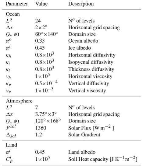
Table 1. Ocean, atmosphere and land main parameters for the
Control experiment. Diffusivity and viscosity values are given in m2s−1. The vertical diffusivityκv parameter will be changed in
the Kv-Experiments. When GM is used the horizontal diffusivity
κhis set to zero.
Parameter Value Description Ocean
Lo 24 Noof levels
1x 2×2◦ Horizontal grid spacing
(λ, φ) 60◦×140◦ Domain size
αo 0.33 Ocean albedo
αi 0.45 Ice albedo
κh 0.8×10³ Horizontal diffusivity κi 0.8×10³ Isopycnal diffusivity κt 0.8×10³ Thickness diffusivity νh 1×10⁵ Horizontal viscosity κv 0.5×10⁻⁴ Vertical diffusivity νv 1×10⁻³ Vertical viscosity
Atmosphere
La 7 Noof levels
1x 3.75◦×3◦ Horizontal grid spacing
(λ, φ) 120◦×168◦ Domain size
Fsol 1360 Solar Flux [W m−2]
1sol 1.2 Solar Gradient
Land
αl 0.45 Land albedo
Cpl 1×10⁵ Soil Heat capacity [J K−1m−2]
However, the benchmark configuration is the one cho-sen to reproduce the observed annual and zonal mean top of the atmosphere (TOA) net shortwave flux, and in that case the solar flux is given by
Fsol= Rsol 4
(
1.0+1sol
(1−3µ2)
4
)
, (1)
whereRsolis the global mean solar flux,1solthe merid-ional solar gradient andµis sine-latitude (see Table 1). For simplicity we also neglect solar absorption in the atmosphere, and we thus rely on surface albedo to rep-resent the total planetary albedo.
weaker mass transport by the Hadley cells and a reduc-tion in the dependency on horizontal resolureduc-tion. Wa-ter vapour itself is a prognostic variable, but there is no liquid water or clouds: liquid water substance all falls to the surface as rain immediately upon condensation, which occurs at saturation and with a corresponding adjustment of temperature, preserving energy (Frierson et al., 2006).
3. A simplified Monin-Obukhov similarity theory for the computation of surface fluxes and a boundary layer scheme linked to the drag coefficients calculation was implemented in order to mediate the boundary layer fluxes in the model.
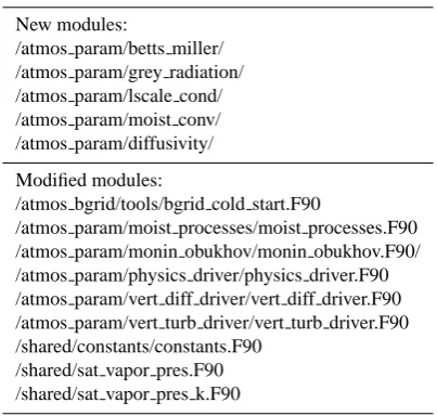
At present, the model does not incorporate trace gases nor clouds, making it unsuitable for climate change stud-ies. However, we envisage in the near future the inclusion of an improved radiation scheme similar to the one devel-oped in Molteni (2003). For a more detailed description of the physical parametrizations we refer the reader to Frierson (2005) (available at: www.atmos.washington.edu/∼dargan/ papers/thesis.pdf). We would like to stress at this point that all model modifications have been implemented in a modular way, that is, it is possible to switch back to the “full-physics” parameterisations with a simple namelist change. Modules that have been modified or added to the FMS B-grid atmo-spheric model are listed in Table 2.
2.3 The land component
The GFDL Land model (LM2.0; Milly and Shmakin, 2002) is implemented as a single “bucket” soil water reservoir. Liq-uid water capacity of each land cell is gathered into a single soil water reservoir, and constant values of water availabil-ity, heat capacavailabil-ity, roughness and drag coefficients are used. Rain can accumulate in the soil to a maximum prescribed soil moisture content (i.e., water availability). When precip-itation exceeds the prescribed water capacity, a very simple basin map collects the precipitated water and idealised rivers redistribute the water back into the ocean at the nearest point. The advantages of such bucket land are the closure of the water budget compared to a swamp and the simplification of land/sea effects on the precipitation-minus-evaporation flux. On the other hand, in some places – notably the equatorial regions – the land reaches high temperatures, which must be damped by an artificially high constant albedo (0.45). Presently there is no orography in the model and glaciers are not allowed to form, as all precipitated water stays in its liq-uid form.
3 The Atlantic configuration
We will firstly present the climate of our most tested and used configuration, where the focus is on a single basin ocean
cou-Table 2. New and modified modules in the B-grid atmospheric
component.
New modules:
/atmos param/betts miller/ /atmos param/grey radiation/ /atmos param/lscale cond/ /atmos param/moist conv/ /atmos param/diffusivity/ Modified modules:
/atmos bgrid/tools/bgrid cold start.F90
/atmos param/moist processes/moist processes.F90 /atmos param/monin obukhov/monin obukhov.F90/ /atmos param/physics driver/physics driver.F90 /atmos param/vert diff driver/vert diff driver.F90 /atmos param/vert turb driver/vert turb driver.F90 /shared/constants/constants.F90
/shared/sat vapor pres.F90 /shared/sat vapor pres k.F90
pled to a sector atmosphere: the Atlantic configuration. Sec-tor coupled models can be very useful in identifying basin-scale processes, air-sea interactions and dynamical responses to local and remote perturbations in the climate system. The kind of idealised model presented here should be used as a tool for testing simple theoretical arguments or complicated responses emerging from CGCMs. The main advantage is the presence of a fully dynamical and interactive atmosphere, which can mediate air-sea fluxes without the need for arti-ficial restorings or applied forcings, and the possibility of performing millennia integrations in a variety of parameter spaces. Within this configuration we have performed a series of multiple millennial coupled experiments in which we vary some geometrical factor or parameter in order to study the difference in the resulting climate, both its steady-state and variability. These experiments are listed in Table 3.
The constant vertical diffusivity in the ocean is set to
κv=0.5×10⁻⁴m2s−1. This value is somewhat larger than
that observed in the main thermocline but smaller values of diffusivity led to a meridional overturning circulation that was weaker than observed (see Fig. 7, but read below for a discussion on this), possibly because the real thermohaline circulation depends on locally large values of diffusivity (for example over rough topography, and in coastal margins e.g., Samelson, 1998). Moreover, to test the role of vertical diffu-sivity in our model and its sensitivity, we performed several experiments whereκv is modified towards both higher and
lower values (for a review on the subject see Kuhlbrodt et al. (2007)). The isopycnal or Redi diffusivity (κi) and isopycnal
thickness diffusivity (κt, skew-flux advection of tracers by
mo-Fig. 1. The oceanic and atmospheric grid in the Atlantic
experi-ment: the ocean basin sits in the centre of the atmospheric sector, spanning 60◦in longitude and from 70◦S to 70◦N. A cyclic chan-nel extends from 65◦S to 51◦S. The atmosphere is 120◦wide with solid meridional walls at 84◦S and 84◦N.
mentum viscosities are set to 1×10⁵and 1×10⁻³m2s−1, re-spectively. These are somewhat higher than might be ideal, but are necessary in low resolution models to smooth out un-physical noise (Fanning and Weaver, 1997). See Table 1 for a complete list of oceanic parameters. For the Atlantic case, we configure the model into a single ocean basin of similar dimensions to the Atlantic Ocean, with a re-entrant southern channel near the southern boundary representing the Antarc-tic Circumpolar Current. In Fig. 1, the ocean domain is filled by the grey area together with its actual grid. The ocean do-main is 60◦wide and has a latitudinal extension from 70◦S to 70◦N. The horizontal resolution is constant and has a nom-inal value of 2.0◦; the vertical discretization consists of 24 levels of increasing thickness towards the bottom, which has a depth of 4000 m and is flat throughout the domain, except in the model Drake Passage, which is 14◦wide between 65◦S and 51◦S and has a reduced depth of 2500 m. No-slip condi-tions at the lateral walls and a drag at the bottom are enforced for horizontal velocities. Cyclic boundary conditions exist in the open channel area.
Since our aim is to study ocean-atmosphere interactions at the basin scale on interannual to centennial time scales, the atmospheric model was configured to run as a zonally re-entrant sector with solid meridional walls. Hence, we have excluded possible inter-basin teleconnections. The resulting geometrical configuration is that of a spherical sector model with no poles. The sector atmospheric B-grid is periodic and 120◦wide. Like the ocean component, it has full spherical geometry and the same radius as the Earth and was coupled
Table 3. Different configurations tested for the sector Atlantic
simu-lation. For each experiment, we state in the column “Specifications” only the differences with the Control experiment CTL. (Kv: verti-cal diffusivity (m2s−1); GM: Gent-McWilliams; HD: Horizontal Diffusion; DP: Drake Passage; NDP: no Drake Passage.)
Name Yrs Specifications Kv005 1000 Kv=0.05e-4 Kv01 1000 Kv=0.1e-4 Kv025 500 Kv=0.25e-4 Kv05 (CTL) 2000 Kv=0.5e-4; GM, DP Kv1 500 Kv=1.0e-4
Kv2 500 Kv=2.0e-4 Kv5 500 Kv=5.0e-4 X2 1000 2×wide Ocean NDP 1000 no Drake Passage HD 1000 Laplacian Diffusivity NoWall 500 No meridional walls
to the ocean and land components through the GFDL FMS exchange grid. The resolution is equivalent to the GFDL M30, corresponding to a nominal horizontal resolution of 3.75◦×3◦, and 7 uneven levels in the vertical.
The geometrical effects have been studied with four ma-jor modifications: the closing of the Drake Passage (NDP), the widening of the oceanic basin (X2), shallowing the basin depth (H) and the removal of the zonal walls rendering the ocean basin a re-entrant channel (NoWall). The oceanic pa-rameters that have been explored are the vertical diffusivity
κv and the parameterisation of horizontal diffusivity (Gent
and McWilliams (GM) vs. Laplacian horizontal diffusivity (HD)). Here we mainly restrict our attention to the Control (CTL) solutions, as the main focus of the present paper is on the description of a base integration. Furthermore, we tested the climatic response to variations of some fundamen-tal parameters of the climate system such as the moisture content in the atmosphere, the meridional gradient of the in-cident solar flux and the Earth’s rotation rate. Various numer-ical experiments and analyses on the climate variability, en-ergy transport in the coupled system and their dependence on oceanic, atmospheric and planetary parameters and dimen-sions will be presented elsewhere. The archived data files and analyses from all of the above mentioned sensitivity in-tegrations can be made available to the interested reader. Coupling procedure
Fig. 2. The wind stress over the ocean for the ICCMp1 model (red
line, Atlantic case) and the GFDL CM2.1 (heavy black line). The other two curves are observational data sets. The major deficien-cies are a too small difference between the Northern and Southern Hemisphere midlatitude jets, and the equatorward position of the Soutehern midlatitude jet.
moisture and momentum are plotted in Figs. 2 and 3, and a list of the main parameters is given in Table 1. The IC-CMp1 momentum, heat and freshwater fluxes compare rea-sonably well with those generated by the present-day GFDL CM2.1 simulation and some reanalysis datasets over the At-lantic region (Figs. 2 and 3). The main deviation is found in the momentum flux, which is too weak and equatorwards in the Southern Hemisphere, although this has been a long standing problem for many atmospheric models in the past.
With the Atlantic configuration and resolution, the atmo-sphere, although highly idealised, takes around 6 times more CPU time than the ocean. Besides being a limitation, this also means that refining the oceanic resolution, or even the addition of a second basin, does not slow down the cou-pled model integration significantly (as we will see later). Presently, the model is capable of performing 15 model years per wallclock hour on 32 processors.
3.1 Mean climate 3.1.1 The ocean
The ocean basin resembles the Atlantic ocean in its geometry and we thus find a roughly similar circulation, except in so far as the presence of other ocean basins influence the circulation of the Atlantic.
The time-mean zonal-mean potential temperature and salinity are shown in Fig. 4. Cold and relatively fresh waters are subducted in the Southern Hemisphere close to the re-entrant channel mimicking the Drake Passage. A reasonably realistic, albeit overly diffusive, thermocline is maintained
Fig. 3. Precipitation-minus-evaporation (PME, top) and surface
to-tal heat flux (SHF, bottom) comparison between the Atlantic IC-CMp1 model (blue line) and the CM2.1 (black line) over the At-lantic ocean.
Fig. 4. Zonal mean potential temperature and salinity for the
At-lantic Control case in whichκvis set to 0.5×10⁻⁴[m2s−1].
Fig. 5. Sea surface temperature (SST), salinity (SSS), heat flux (HF), 100-m-averaged mean oceanic currents and sea-ice thickness in the
Atlantic experiment. The contour interval is 1◦C for temperature, 0.25 psu for salinity and 10 W m−2for the surface heat flux and 0.1 m for sea-ice; a reference velocity arrow is given at the top of the fourth panel for velocity reference.
and subtropical maxima in salinity are present. Experiments with different values ofκv vary substantially in their depth
of the thermocline and abyssal stratification, with CTL being the closest to real Atlantic conditions.
Many aspects of the mean state oceanic conditions can be interpreted from the panels of Fig. 5: an equatorial cold tongue is present, sea-ice concentration is asymmetric be-tween the poles, surface salinity has two major salty limbs in the subtropics and region of freshwater river discharge are visible. Finally the ocean gains heat in the equatorial re-gion (positive flux is into the ocean) and loses heat to the atmosphere at the poles and in the western boundary current areas. The surface circulation presents a subtropical and a subpolar gyre in the Northern Hemisphere while only a sub-tropical gyre exists in the Southern Hemisphere due to the
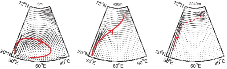
Fig. 6. Surface, mid-depth and deep horizontal circulation. The red arrows are schematics of the main circulation patterns at different depths:
a strong subtropical gyre at the surface; then a western boundary current and northeastward flow at 400 m converging in the northeastern corner of the basin where it is associated with deep convection; and finally, at 2000 m, a southward deep western boundary current and divergent flow in the northeastern boundary.
Fig. 7. The time-mean residual meridional overturning circulation
in Sverdrups (Sv≡106m3/s) in the different coupled experiments for different values of vertical diffusivity (Kv, in×10−4m2s−1), basin width (X2, two times wider), no Drake Passage (NDP, closed basin) and Laplacian horizontal diffusivity (HD, same parameter value as in GM).
of mass transport) for the CTL case. This is shown in Fig. 7 where the time mean residual meridional overturning circula-tion (MOC) is shown in physical space for some of the cou-pled experiments. In the Northern Hemisphere, both buoy-ancy forcing and mechanical energy produce a reasonably re-alistic overturning circulation of∼12 Sv extending to a depth of 2500 m.
Figure 7 also clearly shows the dependency of the MOC on the background vertical diffusivity, both in its spatial struc-ture and magnitude. The northern branch is vanishing for lower values ofκv, while a more symmetrical circulation de-velops with increasing vertical diffusivity due to a stronger southern cell. The wind-driven asymmetry generated by the opening of the Drake passage will eventually become of sec-ond order importance in a diffusively-dominated circulation. Shallow tropical wind-driven cells disappear for sufficiently strong values of κv. As expected, with the closure of the
Drake passage the circulation becomes symmetric around the equator.
The total time mean energy transport in the ocean is ap-proximated by
8o≈ρoCpo
Z
vθdxdz, (2)
whereρoCop is the volumetric specific heat of the ocean,v
Fig. 8. Meridional oceanic heat transport for all different experiments. Top: total transport including neutral physics. Bottom: advection
(heavy lines) and diffusive (light lines) components.
ρoCpoL η
Z
−H
[vθ]dz=ρoCpoL η
Z
−H
[v][θ]dz
| {z }
overturning
(3)
+ρoCpoL η
Z
−H
[v∗θ∗]dz
| {z }
gyre
,
whereLis the width of the basin,Hits total depth andηthe surface elevation.
A qualitative crude comparison of the energy transports in the model and observations will be given later on (see Sect. 3.1.2); here we focus on the oceanic component and its dependency on different parameters. The oceanic energy transport and its decomposition into advective and diffusive parts, as well as the overturning and gyre contributions are shown in Figs. 8 and 9, respectively. In experiments where
κv is varied (right panels of Fig. 8) we clearly see that the
more diffusive the ocean, the more symmetric around the equator the heat flux becomes, consistent with the overturn-ing circulation behaviour. Also, the diffusive transport (thin lines in the bottom panels of Fig. 8) plays a negligible role in all simulations except in the vicinity of the Drake passage,
Fig. 9. Meridional oceanic heat transport for the Control (CTL)
case (κv=0.5×10⁻⁴). Advection (black), Overturning (blue) and
Gyre (red) component.
Fig. 10. Zonal mean atmospheric potential temperature2, zonal windU, humidityqand mass streamfunctionψain the sector atmosphere.
The jet is stronger in the Southern Hemisphere and projects onto stronger surface westerlies; the southern Hadley cell is also stronger and penetrates across the equator. From the depth of the Ferrel cells we can see that the planetary boundary layer is very deep due to relative too warm land over half of the domain. Note that there is no seasonal cycle in the model.
heat transfer is driven by the deep overturning circulation, the Ekman transport and associated shallow cell at low lati-tudes, and by mesoscale eddies, which are parameterised in our integrations. While in the CTL case the mesoscale eddy parameterisation (the GM term) makes almost no direct con-tribution to the energy transport, in the case with no merid-ional walls the isopycnals are almost vertical and the GM contribution is large, consistent with the results of Marshall et al. (2007) (see also later for our Aquaworld configuration). Finally, for all experiments the meridional energy trans-port is dominated by the overturning component (Fig. 9), while the gyre component is significant only at high latitudes or in the Southern Hemisphere, where the heat flux is rela-tively small.
3.1.2 The atmosphere
As we have noted in Sect. 2, the main simplifications in the ocean model are geometrical while the atmospheric compo-nent has important idealisations and omissions in its physical processes, and we therefore might expect a greater deviation from the climatology of a state-of-the-art atmospheric model. Nonetheless, we do find a qualitatively and, in some aspects, quantitatively realistic atmospheric circulation.
The zonal mean atmosphere is summarised in Fig. 10 where potential temperature, zonal winds, humidity and mass stream function are plotted. The model exhibits a fairly real-istic pattern from low to high latitudes with somewhat weak
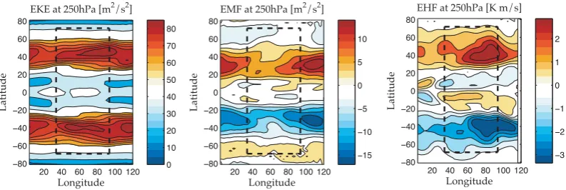
hemispheric asymmetry, with stronger surface westerlies and lower values of humidity in the Southern Hemisphere due to more sea-ice there. The westerly jets at mid-latitudes are the regions of maxima in the eddy kinetic energy correspond-ing to our “storm tracks” and downstream eddy momentum fluxes (see Fig. 12). The atmospheric circulation possesses a Hadley cell with a maximum mass transport of 150 Sv, weaker Ferrel cells of about 20 Sv and some poorly resolved polar cells.
8a=
Z
(CpaT +gz+Lq)v/gdpdx, (4)
wherev is the meridional component of the total velocity,
Cpais the specific heat capacity of the atmosphere,T its tem-perature,gzthe geopotential height, Lis the latent heat of condensation andq is the specific humidity. From Fig. 11 we see how the dry static energy (DSE=CpT+gz)
compen-sates the equatorward latent transport of moisture (LE=Lq) in the Hadley cell region and the latitude of maximum total flux (PHT in Fig. 11) is about 37 degrees, consistent with ob-servations (Trenberth and Caron, 2001). A primary deviation from observational estimates is in the ratio between DSE and LE in the present configuration, which is about twice as much as in the observations of Trenberth and Stepaniak (2003), and is mostly due to lower humidity contents over land and the high land fraction throughout the domain.
Overall, with the given differential solar heating, the ide-alised coupled model is capable of reproducing a fairly re-alistic climate in both the ocean and atmosphere, given the caveats appropriate for a simplified model. The model’s ide-alisations keep the system simple enough as to highlight the main mechanisms of interaction between the ocean and at-mosphere at interannual and longer time scales, but at the same time do not oversimplify to the point of unrealism. 3.1.3 Sea-ice
The sea-ice climatology is, as expected, asymmetric around the equator because of the presence of the Drake Passage and the resulting meridional heat flux in the ocean. As in real Atlantic ocean conditions, more sea-ice is generated down-stream the Antarctic peninsula (represented here by the wall on the South West corner of the domain) extending all the way to the eastern end of the Atlantic Ocean. In the North-ern Hemisphere, sea-ice is concentrated in the North West corner, possibly because of the cold continental air flowing easterly and the effect of the subpolar gyre advecting warm water to the North eastern corner of the ocean basin (Fig. 5, right panel).
4 The Aquaworld configuration
The ICCMp1 is not restricted to a sector configuration, and the natural generalization is that of a “full-Earth” geome-try (called here Aquaworld), where a spherical atmosphere is exchanging freshwater, heat and momentum fluxes with an Earth that is totally covered by water with the only ex-ception of two polar caps that are necessary for the sea-ice model. The coupled model now resembles the configurations of Smith et al. (2006) and Marshall et al. (2007), the only other modelling initiatives where a dynamical atmosphere is coupled to a dynamic ocean with no continents. With respect
Fig. 11. Top panel: planetary (PHT), atmospheric (AHT) and oceanic (OHT) heat transport for the sector Atlantic model. Lower panel: AHT or moist static energy (MSE=CpT +gz+Lvq), dry
static energy (DSE=CpT+gz) and latent energy (LE=Lvq) in the
CTL simulation.
to the Atlantic experiment, only geometrical differences exist in the case of the Aquaworld model, and all other parameters and model characteristics have remained constant. Also, the model is now roughly only three times slower, as most of the CPU time is taken up by the atmosphere.
Fig. 12. Eddy Kinetic Energy (EKE), Eddy momentum flux (EMF) and Eddy heat flux (EHF) at 250 hPa for the Atlantic CTL experiment.
The dotted squared box represents the ocean basin.
Fig. 13. Some oceanic fields during spin-up of the Aquaworld experiment. From top left: sea surface temperature (SST), sea surface salinity
(SSS), sea-ice thickness (HI) in meters, zonal wind stress (Taux) in N m−2, precipitation minus evaporation (PmE) in mm day−1and the total surface heat flux (SHF) in W m−2. The polar islands can be seen in some of the plots.
can be no zonally-averaged geostrophic flow in the interior. Any net meridional Ekman transport at the surface cannot be returned in the ocean interior and all the cells return in a bottom boundary layer; hence, there is no hemispheric-scale meridional overturning circulation in the ocean (not shown). Whilst the oceanic resolution is too coarse to re-solve the small oceanic Rossby radii (hence mesoscale pro-cesses have to be parameterised) the radius of deformation in the atmosphere is much larger and so synoptic scale sys-tems arise naturally. To demonstrate this, some daily snap-shots are given in Fig. 15, where rich structures are clearly visible, especially in the mid-latitudes. How the meridional
energy transport is partitioned between the two fluids in the
Aquaworld model is illustrated in Fig. 16. Basic features
are the symmetry of the transport around the equator, the larger transport accomplished by the ocean at very low lat-itudes and the dominance of the atmosphere at mid and high latitudes. As in the Atlantic experiment with no meridional walls (NoWall), the eddy-induced (bolus) transport opposes the eulerian transport giving rise to a total transport that is polewards at all latitudes.
exper-Latitude Pressure 275 300 350 425 325 T [K]
80S 60S 40S 20S 0 20N 40N 60N 80N 200
400
600
800
Latitude
Depth (m) 0
4 8 12 16 20 24 26 22 18 14 10 6 T[C]
80S 60S 40S 20S 0 20N 40N 60N 80N 1000 2000 3000 Latitude Pressure 107 5 3 21 4 7 9 q [g/kg]
80S 60S 40S 20S 0 20N 40N 60N 80N 200 400 600 800 Latitude Depth (m) 36.25 35.75 35.25 35.75 35.25 35 34.75 34 34.5 36.25 S[psu]
80S 60S 40S 20S 0 20N 40N 60N 80N 1000
2000
3000
Fig. 14. Zonal mean atmospheric and oceanic structure during spin-up of the Aquaworld experiment. In the top panels are the
atmo-spheric potential temperature (CI=25◦K) and relative humidity (CI=1 g/Kg) while the bottom panels show the oceanic potential temperature (CI=2◦C ) and salinity (CI=0.5 psu).
iments. Hence the Aquaworld model is a useful tool for studies of the partition and sensitivity of the heat transport in both the atmosphere and ocean subject to different per-turbations. The model is totally flexible to changes in its basic geometrical configuration and sets of parameters and parameterisations; the two experiments presented in this pa-per should be regarded as mere examples of many possible configurations. For example, the ocean circulation can be re-stricted by the incorporation of one or more walls that would block the flow and set-up a gyre circulation and western boundary currents, giving rise to many different climatic re-sponses. Although these experiments might seem extremely idealised, they not only give much insight into the dynamics of ocean-atmosphere interactions for the climate of the Earth in present day conditions (Marshall et al., 2007) but also serve as a useful test for paleoclimate circulations, biogeo-chemical processes and dependencies on geometrical factors on both circulations and air-sea exchanges. Some of these ideas are presently been applied to the model with a suite of
Aquaworld configurations.
5 Summary and discussion
In this paper we have described the ICCMp1, an intermediate complexity climate model based on the GFDL FMS.
Fig. 15. Daily snapshot of some atmospheric fields for the
Aqua-world experiment. From top left: convectively available potential
energy (CAPE), specific humidity (q) at 500 mb, outgoing long-wave radiation (OLR), geopotential height (8) at 500 mb, relative vorticity (ζ) at 500 mb and sea level pressure (SLP).
reproduce a reasonably realistic circulation in both the at-mosphere and ocean, with the latter being very similar to an Atlantic-like climate in its control simulation. Sensitivity to a set of parameter values and geometrical settings was also briefly discussed.
One purpose of using such a model is to provide a pathway between reality and theory because GCMs in realistic ge-ometries (which in turn are much less complex than the real ocean-atmosphere system) are generally too complicated to allow straightforward application of many theoretical ideas. The presence of topography and non-regular basin shapes, for example, means that classical ideas from ocean dynam-ics are hard to apply, and the complications of clouds in the atmosphere make the interpretation of the effects of mois-ture very difficult. By using simpler models we hope that the connection to theory may be made more directly, yet by us-ing the primitive equations with all the dynamics of climate models we avoid the oversimplications of still more
idealiza-Fig. 16. Meridional heat transports in the Aquaworld experiment.
The oceanic (OHT) and atmospheric (AHT) heat transports sum up to give a total, or planetary (PHT), transport of about 6 PW (1 PW≡1015W) in each hemisphere. The oceanic decomposition into an eulerian and eddy-driven or bolus component is shown in the bottom panel.
tions such as quasi-geostrophic models. Smith et al. (2006) and Marshall et al. (2007) used idealised coupled frameworks in a similar spirit.
Finally, we believe that ICCMp1 is a powerful tool for the study of ocean-atmosphere interactions and variability from interannual to centennial periods, with a close connection to the Earth’s present day, and possibly past, climate. Also, ocean modellers might find useful to study the ocean and sea-ice components of the climate system when coupled to a simple, fast and yet dynamically interactive atmosphere. Acknowledgements. We would like to thank Dargan Frierson
for developing the simplified atmospheric physics packages, Stephen Garner for help with the Atmospheric model, and Chris Milly and Sergey Malyshev for assistance with the Land model. A special thanks to Stephen Griffies for his help and advice on Ocean modelling and development. Two anonymous reviewers provided useful suggestions to improve the paper. This work was funded by NOAA and NSF. RF was supported by the GFDL/AOS Postdoctoral Program.
References
Betts, A. K.: A new convective adjustment scheme. Part I: Obser-vational and theoretical basis, Q. J. Roy. Meteorol. Soc., 112, 677–692, 1986.
Betts, A. K. and Miller, M. J.: A new convective adjustment scheme. Part II: Single column tests using GATE wave, BOMEX, and arctic air-mass data sets, Q. J. Roy. Meteorol. Soc., 112, 693– 709, 1986.
Delworth, T., Broccoli, A., Rosati, A., Stouffer, R., Balaji, V., Beesley, J., Cooke, W., Dixon, K., Dunne, J., Dunne, K., Du-rachta, J., Findell, K., Ginoux, P., Gnanadesikan, A., Gordon, C., Griffies, S., Gudegel, R., Harrison, M., Held, I., Hemler, R., Horowitz, L., Klein, S., Knutson, T., Kushner, P., Langen-horst, A., Lee, H.-C., Lin, S., Lu, L., Malyshev, S., Milly, P., Ramaswamy, V., Russel, J., Schwarxkopf, M., Shevliakova, E., Sirutis, J., Spelman, M., Stern, W., Winton, M., Wittenberg, A., Wyman, B., Zeng, F., and Zhang, R.: GFDL’s CM2 global cou-pled climate models. Part I: Formulation and simulation charac-teristics, J. Climate, 19, 643–674, 2006.
Enderton, D. and Marshall, J.: Controls on the total dynamical heat transport of the atmosphere and oceans, J. Atmos. Sci., 66, 1593– 1611, 2009.
Fanning, A. F. and Weaver, A. J.: A horizontal resolution and pa-rameter sensitivity study of heat transport in an idealized coupled climate model, J. Climate, 10, 2469–2478, 1997.
Frierson, D. M. W.: Studies of the general circulation of the atmo-sphere with a simplified moist general circulation model, Ph.D. thesis, 2005.
Frierson, D. M. W.: The Dynamics of Idealized Convection Schemes and Their Effect on the Zonally Averaged Tropical Cir-culation, J. Atmos. Sci., 64, 1959–1976, 2007.
Frierson, D. M. W., Held, I. M., and Zurita-Gotor, P.: A Gray-Radiation Aquaplanet Moist GCM. Part I: Static Stability and Eddy Scales, J. Atmos. Sci., 63, 2548–2566, 2006.
Frierson, D. M. W., Held, I. M., and Zurita-Gotor, P.: A gray-radiation aquaplanet moist GCM. Part II: Energy transports in altered climates, J. Atmos. Sci., 64, 1680–1693, 2007.
Garner, S. T., Frierson, D. M. W., Held, I. M., Paulius, O. M., and Vallis, G. K.: Resolving convection in a global hypohydrostatic model, J. Atmos. Sci., 64, 2061–2075, 2007.
Gent, P. and McWilliams, J.: Isopycnal mixing in ocean circulation models, J. Phys. Oceanogr., 20, 150–155, 1990.
Griffies, S.: The Gent-McWilliams skew-flux, J. Phys. Oceanogr., 28, 831–841, 1998.
Griffies, S. M., Harrison, M. J., Pacanowski, R. C., and Rosati, A.: A technical guide to MOM4, Tech. Rep. GFDL Ocean Group No. 5, 2004.
Griffies, S. M., Gnanadesikan, A., Dixon, K. W., Dunne, J. P., Gerdes, R., Harrison, M. J., Rosati, A., Russell, J. L., Samuels, B. L., Spelman, M. J., Winton, M., and Zhang, R.: Formulation of an ocean model for global climate simulations, Ocean Sci., 1, 45–79, 2005,
http://www.ocean-sci.net/1/45/2005/.
Hazeleger, W., Severijns, C., Haarsma, R., Selten, F., and Sterl, A.: SPEEDO – model description and validation of a flexible coupled model for climate studies, Tech. Rep. TR-257, 37 pp., 2003.
Held, I. M.: The Gap between Simulation and Understanding in Climate Modeling, B. Am. Meteorol. Soc., 86, 1609–1614, 2005. Hogg, A., Dewar, W., Killworth, P., and Blundell, J.: A quasi-geostrophic coupled model: Q-GCM, Mon. Weather Rev., 131, 2261–2278, 2003.
Kamenkovich, I. V., Marotzke, J., and Stone, P. H.: Factors affect-ing heat transport in an ocean general circulation model, J. Phys. Oceanogr., 30, 175–194, 2000a.
Kamenkovich, I. V., Sokolov, A. P., and Stone, P. H.: A coupled atmosphere-ocean model of intermediate complexity for climate change study, Tech. Rep. No.60, 2000b.
Kamenkovich, I. V., Sokolov, A. P., and Stone, P. H.: An efficient climate model with a 3D ocean and a statistical-dynamical atmo-sphere, Clim. Dynam., 19, 585–598, 2002.
Kravtsov, S. and Ghil, M.: Interdecadal variability in a hybrid cou-pled ocean-atmosphere-sea-ice model, J. Phys. Oceanogr., 34, 1756–1775, 2004.
Kravtsov, S. and Robertson, A.: Midlatitude ocean-atmosphere in-teraction in an idealized coupled model, Clima. Dynam., 19, 693–711, 2002.
Kravtsov, S., Dewar, W. K., Berloff, P., McWilliams, J. C., and Ghil, M.: A highly nonlinear coupled mode of decadal variability in a mid-latitude ocean-atmosphere model, Dynam. Atmos. Oceans, 43(3–4), 123–150, 2007.
Kuhlbrodt, T., Griesel, A., Montoya, M., Levermann, A., Hofmann, A., and Rahmstorf, S.: On the driving processes of the Atlantic meridional overturning circulation, Rev. Geophys., 45, RG2001, doi:10.1029/2004RG000166, 2007.
Marshall, J., Ferreira, D., Campin, J. M., and Enderton, D.: Mean climate and variability of the atmosphere and ocean on an aqua-planet, J. Atmos. Sci., 64, 4270–4286, 2007.
Milly, P. C. D. and Shmakin, A. B.: Global modeling of land water and energy balances. Part I: The land dynamics (LaD) model, J. Hydrometeorol., 3, 283–299, 2002.
Mitchell, J. L., Pierrehumbert, R. T., Frierson, D. M. W., and Ca-ballero, R.: The dynamics behind Titan’s methane clouds, P. Natl. Acad. Sci., 103, 18421–18426, 2006.
of intermediate complexity CLIMBER-3α. Part I: description and performance for present-day conditions, Clim. Dynam., 25, 237–263, 2005.
Opsteegh, J., Haarsma, R., Selten, F., and Kattenberg, A.: ECBILT, a dynamical alternative to mixed boundary conditions in ocean models, Tellus, 50A, 348–367, 1998.
Samelson, R. M.: Large-scale circulation with locally enhanced ver-tical mixing, J. Phys. Oceanogr., 28, 712–726, 1998.
Saravanan, R. and McWilliams, J. C.: Multiple equilibria, nat-ural variability, and climate transitions in an idealized ocean-atmsophere model, J. Climate, 8, 2296–2323, 1995.
Saravanan, R. and McWilliams, J. C.: Stochasticity and spatial reso-nance in interdecadal climate fluctuations, J. Climate, 10, 2299– 2320, 1997.
Smith, R. S., Dubois, C., and Marotzke, J.: Global climate and ocean circulation on an aquaplanet ocean-atmosphere general circulation model, J. Climate, 19, 4719–4737, 2006.
Smith, R. S., Gregory, J. M., and Osprey, A.: A description of the FAMOUS (version XDBUA) climate model and control run, Geosci. Model Dev., 1, 53–68, 2008.
The GFDL Global Atmospheric Model Development Team: The New GFDL Global Atmosphere and Land Model AM2-LM2: Evaluation with Prescribed SST Simulations, J. Climate, 17, 4641–4673, 2005.
Trenberth, K. and Caron, J. M.: Estimates of meridional atmosphere and ocean heat transports, J. Climate, 14, 3433–3443, 2001. Trenberth, K. E. and Stepaniak, D. P.: Covariability of
compo-nents of poleward energy transports on seasonal and interannual timescales, J. Climate, 16, 3691–3705, 2003.