Unbiased Generative Semi-Supervised Learning
Patrick Fox-Roberts∗ [email protected]
Cambridge University Engineering Department Trumpington Street
Cambridge, CB2 1PZ, UK
Edward Rosten [email protected]
Computer Vision Consulting 7th floor
14 Bonhill Street
London, EC2A 4BX, UK
Editor:William Cohen
Abstract
Reliable semi-supervised learning, where a small amount of labelled data is complemented by a large body of unlabelled data, has been a long-standing goal of the machine learning community. However, while it seems intuitively obvious that unlabelled data can aid the learning process, in practise its performance has often been disappointing. We investigate this by examining generative maximum likelihood semi-supervised learning and derive novel upper and lower bounds on the degree of bias introduced by the unlabelled data. These bounds improve upon those provided in previous work, and are specifically applicable to the challenging case where the model is unable to exactly fit to the underlying distribution a situation which is common in practise, but for which fewer guarantees of semi-supervised performance have been found. Inspired by this new framework for analysing bounds, we propose a new, simple reweighing scheme which provides a provably unbiased estimator for arbitrary model/distribution pairs—an unusual property for a semi-supervised algorithm. This reweighing introduces no additional computational complexity and can be applied to very many models. Additionally, we provide specific conditions demonstrating the circum-stance under which the unlabelled data will lower the estimator variance, thereby improving convergence.
Keywords: Kullback-Leibler, semi-supervised, asymptotic bounds, bias, generative model
1. Introduction
Reliable semi-supervised learning has been a long standing goal of the machine learning community. Its desirability is motivated by the observation that when collecting data sets, often each sample has two distinct parts: some feature X, collected from some real world population, often consisting of one or more basic measurements; and some label Y, assigned by the experimenter, representing a higher level concept. Furthermore the act of assigning this higher level label very often constitutes a major bottleneck in the data set creation process. It is perhaps expensive (requiring an expert’s opinion), slow (requiring
an investment of time or staff), or in some way destructive (requiring a component to be tested to destruction, or the death of a patient).
If we wish to fit a model parametrised by some set of parameters θto this distribution, we will need some data setDLconsisting of NL labelled samples,DL= (xi, yi)i=1,...,NL, to train our model with; for example, if we are training using maximum likelihood, we must find the parameters which maximise P(DL|θ), which for iid data is equivalent to finding
θ?= arg max θ
NL X
i=1
log (P(xi, yi|θ)). (1)
In order to get a solution which generalises well to unseen data NL may have to be quite large, especially if the model is rich or the feature space X high dimensional.
A far preferable situation would be to be able to utilise a smaller labelled data set DL, augmented with an additional data set DU consisting of NU unlabelled samples, DU = (xi)i=NL+1,...,NL+NU, which consist only of their observed feature rather than a feature -label pair. In essence the un-labelled data is used to ‘bootstrap’ the -labelled. Un-labelled samples tell us the shape of our distribution in the feature space, while labelled samples give us the classification information.
At first glance, utilising unlabelled data to aid in fitting the parameters of some model appears trivial. Inspired by the likelihood principal (Jaynes, 2003), it is tempting to simply augment the likelihood function of the parameters,P(DL|θ), with the additional unlabelled data,P(DL, DU|θ), and proceed with training exactly as before, that is, find the parameters
θ?S= arg max θ
NL X
i=1
log (P(xi, yi|θ)) + NL+NU
X
i=NL
log (P(xi|θ)). (2)
In practice however this has proven to give mixed results, sometime improving model fitting, other times worsening it. This unpredictable of performance has formed a very major barrier to more widespread adoption of semi-supervised techniques. Many alternative algorithms have been developed to counter this. However, there still exists a need to better understand and quantify why more standard methods fail.
This paper examines the effect of including unlabelled data in a training set when per-forming maximum likelihood fitting of generative models. In particular, it is well known (see, for example, Bishop, 2006) that maximising the parameter likelihood for labelled data approximately minimises the Kullback Leibler divergence between the parametric distribu-tion P(X, Y|θ) and the underlying distribution the data is sampled from, P(X, Y). We show that maximising the likelihood of a data set containing unlabelled samples minimises a different divergence. We then show that the possible error between this and the cor-rect divergence may grow rapidly with the proportion of unlabelled data, and will do so monotonically.
are used in the fields of computer vision and text analysis, both of which could potentially benefit from better semi-supervised algorithms; recent examples of such work include that of Rauschert and Collins (2012), Beecks et al. (2011), L¨ucke and Eggert (2010), Kang et al. (2012) and Zhuang et al. (2012). In the general case there is also evidence that generative models can converge faster than discriminative, as shown by Ng and Jordan (2002), and so are valuable when dealing with small data sets.
2. Previous Work
A great deal of work has been done proposing algorithms designed to take advantage of semi-supervised data. Here we shall concern ourselves instead with examining the work done on finding general bounds on performance.
We begin by considering the highly influential work by Castelli and Cover (1995, 1996). This looks not at a particular semi-supervised algorithm, but rather at a slightly more general question of when unlabelled samples can be of value. They conclude that for an identifiable (as defined in the paper) binary decision problem, using a generative model, the misclassification risk decreases exponentially fast towards the Bayes error as the number of labelled samples increases. This result is encouraging. However, the requirement of identifiability is a strict one. In practise it cannot often be guaranteed, and may even be flatly contradicted.
The work of Dillon et al. (2010) builds upon this. Amongst other things they confirm that provided a data set is generated from P(X, Y|θ0) whereθ0∈Ω, the estimator
ˆ
θN = arg max θ∈Ω
NL X
i=1
log(P(xi, yi|θ)) + N X
i=NL+1
log(P(xi|θ))
is consistent. As such, in cases where there is good reason to believe the true distribution is drawn from the same family as our parametric model, we can expect consistent convergence. They also provide one of few examinations of the associated variance of an estimator, though again under the assumption of an identifiable model.
In a similar vein Zhang (2000) examines the fisher information matrix when learning parameters for semi-supervised learning, and conclude that even when their true distribution can not be expressed by the model parameters being fitted, unlabelled samples always aid in learning in that they reduce the variance of the estimator. From this work we can conclude that adding unlabelled samples is not preventing consistent convergence. As such, if performance is observed to often worsen instead of improve as the number of unlabelled samples increases, the fault must lie elsewhere.
The asymptotic behaviours of semi-supervised learning where the model is mis-specified has been further studied by Cozman et al. (2003); Cozman and Cohen (2006, 2002), where no assumptions are made about the parametric model being close to the underlying dis-tribution. In particular, they show that the limiting value of the optimum parameters θ?
when performing ML semi-supervised learning in such a scenario is
arg max θ
(1−λ)EP(X,Y)(logP(x, y|θ)) +λEP(x)(log(P(x|θ)))
rate. In the limit, as λ→ 1, we will tend towards the solution found training entirely on unlabelled data. They argue that with a few assumptions on the modelling densities, θ?
is a continuous function of λ. They also show that an instance where the asymptotically optimal parameters are not changed byλcomes, as might be expected, when the model is “correct” and can be fitted exactly to the underlying distribution (i.e., the true distribution
P(x, y) is a member of the family of distributions that can be modelled by P(x, y|θ)). The relative value of labelled/unlabelled samples was also investigated in Ratsaby and Venkatesh (1995) for the case of classifying between two multivariate gaussian distributions of unknown class prior and position parameters. As in the work by Castelli and Cover, an exponential decrease in error rate with the number of labelled samples is shown, and an only polynomial decrease in the same with the number of unlabelled samples. However they also demonstrate a deleterious effect in the dimensionality of the space, indicating unlabelled samples are likely to be less useful in high dimensional spaces. Separately, the work of Shahshahani and Landgrebe (1994) examines learning the parameters of both a single gaussian and a GMM when labels are missing. They too note an interesting effect of dimensionality on semi-supervised learning, in particular from the point of view of the Hughes phenomenon (Hughes, 1968). This is the observation that, in theory, increasing the dimensionality of a classification problem by taking new measurements should never increase the Bayes error; yet in practise, if we are learning from sampled data we find performance will after a while degrade due to the larger number of parameters that must be estimated (this is very closely linked to the perhaps more familiarCurse of Dimensionality, see Bishop, 2006). They propose that semi-supervised learning can help mitigate this, but only if the rate of introduction of bias due to the unlabelled samples is lower than the decrease in variance of the estimator.
Recently, Yang and Priebe (2011) has provided an investigation of semi-supervised gen-erative learning that builds upon these conclusions. The key parameters they identify are the asymptotic optima achieved when performing fully supervised learning,θsup∗ , and those achieved from entirely un-supervised learning,θunsup∗ . Provided that the ratio ofNL toN tends towards 0 as N tends towards infinity (where N = NL+NU) we have the scenario where we are moving from a high-variance, unbiased estimate, towards a low variance, bi-ased estimate. Interestingly, the KL divergences between the distributions defined by θ∗sup
andθunsup∗ , and between these distributions and a given estimate based on a data set (either fully labelled or a mixture of labelled and unlabelled), are identified as providing bounds on the probability that classification performance will improve/worsen as unlabelled data is added. Intuitively, if the divergence between the models specified by θ∗sup and θunsup∗ is small, then adding unlabelled data is less likely to significantly worsen results. They also show for a particular model that the point at which this occurs can be quite sharp. How-ever, as it is likely to be different for different models and distributions, it still remains an open question how it can be best estimated.
2.1 Non-ML Algorithms
Given the problems associated with standard ML semi-supervised learning, as well as the desire to utilise unlabelled samples in non-generative models, a large number of alternative objective functions have been proposed to take advantage of unlabelled data. Notable exam-ples include Multi Conditional Learning (introduced by McCallum et al. 2006 and applied to semi-supervised learning by Druck et al. 2007 ) and the hybrid Bayesian approach of Lasserre et al. (2006), both of which utilise mixtures of generative and discriminative mod-els; information theory based approaches, which consider the similarity of class predictions across the kNN graph such as Subramanya and Bilmes (2009, 2008), the mutual information of samples within local clusters (Szummer and Jaakkola, 2002), or the conditional entropy of class predictions across the unlabelled samples (Grandvalet and Bengio, 2006); Expecta-tion RegularisaExpecta-tion (Mann and McCallum, 2007), which seeks to enforce class proporExpecta-tion constraints; Co-training, (Blum and Mitchell, 1998), which makes use of situations where data is known to be separable in two different ‘views’; transduction, (Vapnik, 1998), and the transductive support vector machine; kernel methods, such as those investigated by Krishnapuram et al. (2005) and Jaakkola and Haussler (1999), which seek to use unlabelled samples to build better kernel functions; and many others. A thorough literature review was carried out by Zhu (2005).
3. Local And Global Bounds On Semi-Supervised Divergences
We now present a number of theorems, showing the asymptotic limits of the performance of models trained on semi-supervised data using the standard technique Equation (2). While it has been previously noted in the literature that ML semi-supervised learning introduces bias when the model and underlying distributions do not match, we provide new bounds on the degree of this bias as a function of the proportion of unlabelled data, and the best case performance of our model if it were to be trained on a large labelled data set, giving new insight into the reason behind these bounds.
3.1 Notation And Conditions
A semi-supervised data set consists of two types of data - labelled samples drawn from
P(X, Y), and unlabelled drawn from P(X). To allow us to deal with both of these within a single framework we shall introduce a new variableZ, and consider ourentire data set to be drawn from P(X, Z), {xi, zi}i=1,...N in the space X × Z. We shall allow the ‘labelling’ Z to take on the same set of values asY, plus one extra,U, and thereforeZ =Y ∪U. For every “labelled” sample,zi =yi, and for every “unlabelled” samplezi=U. As such we now have the data set {xi, zi}i=1,...N. Similarly, we shall consider our parametersθto specify a distribution P(X, Z|θ) rather thanP(X, Y|θ), in a manner which will become clear as we proceed.
Condition 1 X is conditionally independent of Z given Y — if we know the class y of samplex, z gives us no more information, that is,
P(x|y, z, θ) =P(x|y, θ), P(x|y, z) =P(x|y)
This first condition represents the fact that zi can be considered a noisy estimate of yi - in as much as it will either be equal to yi, or it will take on the value U to indicateyi is unknown. In either case, if we had access to the true value ofyi, thenzi would be irrelevant as it can give us no useful information. This condition is similar to the “missing at random” assumption discussed by Grandvalet and Bengio (2006).
Condition 2 The labelled samples have been drawn randomly and labelled correctly. The unlabelled samples are similarly drawn randomly, with no class bias. As such,
P(z|y, θ) =
P(U|θ), z=U δk(z, y)P( ¯U|θ), z6=U
P(z|y) =
P(U), z=U δk(z, y)P( ¯U), z6=U
whereδk indicates the Kronecker delta function, and we have denoted1−P(U|θ) asP( ¯U|θ) and 1−P(U) as P( ¯U)
This second condition specifies our labelling process. It is imagined that a ‘bag’ full of unlabelled samples initially exists, and individual ones are then drawn from it and the correct label associated with them by some expensive labelling process1 to form the labelled set.
In practise truly drawing samples completely at random runs with risk of certain classes having zero labelled samples, which is likely to cause highly undesirable behaviour of the algorithm. We do not foresee this as a problem for two reasons. Firstly, in the asymptotic limit (which is what most of our work will be concerned with in this section) we will almost surely achieve labelled samples being drawn from all classes. Secondly, in practise, the indi-viduals running the experiment are likely to ensure that all classes have some representative samples. This breaks the assumption of iid data; however, provided the class priors are re-spected when choosing how many samples to label from each class (or suitable weighting applied) we can still attain an asymptotically unbiased estimate of the expectation term in the divergence.
Condition 3 The proportion of labelled data is known, letting us set P( ¯U|θ) = P( ¯U) = 1−P(U)
We assume this as matching labels to samples is a process controlled entirely by the user, and that they use this knowledge to set P(U|θ) rather than having to infer it from the data.
3.1.1 Divergences
The KL divergence is a widely used method of measuring the similarity between two dis-tributions, and one which shall be made extensive use of in this article. For distributions
P(X, Y) and P(X, Y|θ) where X is a continuous random variable and Y is discrete, it is defined as
KL(P(X, Y)||P(X, Y|θ)) = Z
x∈X X
y∈Y
P(x, y) log
P(x, y)
P(x, y|θ)
It is perhaps most widely used as a justification of maximum likelihood methods, as it is a standard proof that the parameters
θ? = arg max θ
NL X
i=1
log (p(xi, yi|θ))
are an asymptotically unbiased minimiser of KL(P(X, Y)||P(X, Y|θ)), for example, see Bishop (2006).
For brevity and to make subsequent equations more readable we shall introduce a more concise notation to refer to theKLdivergence. For random variablesA andB and param-etersθ, the full divergence shall be denoted as
D(P(A, B), θ)≡KL(P(A, B)||P(A, B|θ))
and the conditional divergence as
D(P(A|B), θ)≡KL(P(A|B)||P(A|B, θ)).
3.2 Standard ML Semi-Supervised Learning Expressed As A Divergence
Our first step is to demonstrate that when a proportion of a data set whose likelihood we are maximising is lacking labels, in the asymptotic limit we will minimise a different divergence to that we might wish - specifically, we minimiseD(P(X, Z)|θ) rather thanD(P(X, Y)|θ).
Theorem 4 Subject to the conditions in 3.1, maximising NL
Y
i=1
P(xi, yi|θ) NL+NU
Y
i=nL+1
P(xi|θ) (3)
w.r.t. θ minimises an asymptotically unbiased estimate of a term directly proportional to
D(P(X, Z), θ), not D(P(X, Y), θ)
Proof Given a set of N samples{xi, zi}i=1,...N drawn from P(X, Z), we can approximate the expectation term in D(P(X, Z)|θ) with an arithmetic mean over our samples (for ex-ample, see MacKay, 2003). Ignoring terms which are not a function of θ, and taking the antilog, we attain
arg min θ
D(P(X, Z), θ)≈arg max θ
N Y
i=1
Examining the above, and making use of Condition 1 to simplify P(xi|zi, y, θ) into P(xi|y, θ), we can rewrite the likelihood contribution of a single sample i, P(xi, zi|θ) as follows
P(xi, zi|θ) = X
y∈Y
P(xi, zi, y|θ)
= X
y∈Y
P(xi|zi, y, θ)P(zi|y, θ)P(y|θ)
= X
y∈Y
P(xi|y, θ)P(zi|y, θ)P(y|θ)
= X
y∈Y
P(xi, y|θ)P(zi|y, θ).
This can be simplified further using Conditions 2 and 3, depending on the value ofzi. First consider the case where zi=U
P(xi, zi|θ)|zi=U = X
y∈Y
P(xi, y|θ)P(U|θ) =P(xi|θ)P(U). (5)
Thus, a sample whose labelling zi indicates it is unlabelled contributes a quantity propor-tional toP(xi|θ) to our likelihood expression. Now consider a single labelled example (i.e., wherezi 6=U),
P(xi, zi|θ)|zi6=U = X
y∈Y
P(xi, y|θ)δk(y, zi)P( ¯U|θ)
= P(xi, y|θ)|y=ziP( ¯U)
= P(xi, yi|θ)P( ¯U) (6)
where we have made a slight change of notation in the last term to represent that ifzi6=U, then yi is known. This contributes a term proportional to P(xi, yi|θ) to the likelihood. If we substitute these results back into Equation (4), our final likelihood expression is
arg max θ
Y
i,zi6=U
P( ¯U)P(xi, yi|θ) Y
j,zj=U
P(U)P(xj|θ)
which is equivalent to maximising Equation (3).
3.3 Bounding D P(X, Y), θ
With D P(X, Z), θ
Maximising the likelihood of a partially labelled data set corresponds to approximately min-imising D(P(X, Z), θ). We now examine how D(P(X, Z), θ) is related to D(P(X, Y), θ), and show that a set of upper and lower bounds can be formed using it.
Theorem 5 Subject to the conditions in 3.1, for a given set of parametersθ,D P(X, Z), θ defines an upper and lower set of bounds on D P(X, Y), θ as follows:
D P(X, Z), θ ≤D P(X, Y), θ≤ D P(X, Z), θ
P( ¯U) . (7)
Remark 6 These bounds imply that, for a givenD P(X, Z), θ that we are optimising, the divergence of interest D P(X, Y), θ could vary by up to a factor P( ¯U)−1. In situations whereP( ¯U)−1 is large, this uncertainty may become the dominant factor in determining the quality of our result.
Proof Consider the KL divergence D(P(X, Z), θ). We shall take the summation over Z
and split out the term z=U, noting thatZ −U =Y
D(P(X, Z), θ) = Z
x∈X X
z∈Y
P(x, z) log
P(x, z)
P(x, z|θ)
dx
+ Z
x∈X
P(x, z)|z=Ulog
P(x, z)|z=U
P(x, z|θ)|z=U
dx.
Using Equation (5) and Equation (6), and their corresponding counterparts when not con-ditioned onθ, we can simplify the terms within our logarithms
P(x, z)|z=U P(x, z|θ)|z=U
= P(x)P(U)
P(x|θ)P(U) =
P(x)
P(x|θ),
P(x, z)|z6=U P(x, z|θ)|z6=U
= P(x, y)|y=z
P(x, y|θ)|y=z.
Using these identities, and Equation (5) and Equation (6) this allows us to rewrite the divergenceD(P(X, Z), θ)
D(P(X, Z), θ) =P( ¯U) Z
x∈X X
z∈Y
P(x, y)|y=zlog P(x, y)|y=z
P(x, y|θ)|y=z
dx
+P(U) Z
x∈X
P(x) log P(x)
P(x|θ)
dx.
which is exactly equivalent to
From this we can find a set of upper and lower bounds on D(P(X, Y), θ) in terms of
D(P(X, Z), θ) alone. The upper bound can be found by noting D(P(X), θ) ≥ 0, which given Equation (8) implies
D(P(X, Z), θ)≥P( ¯U)D P(X, Y), θ
(9)
which when rearranged gives the upper bound in Equation (7). The lower bound follows similarly, by noting that D(P(X, Y), θ) = D(P(Y|X), θ) +D(P(X), θ) ≥ D(P(X), θ). Again using Equation (8) this gives
D(P(X, Z), θ) ≤ P( ¯U)D P(X, Y), θ+P(U)D P(X, Y), θ
= P( ¯U) +P(U)D P(X, Y), θ
= D P(X, Y), θ (10)
which gives us our lower bound. Combining Equation (10) and Equation (9) gives us Equa-tion (7).
It is notable that in deriving these bounds we have treatedD(P(X), θ)) (or, equivalently,
D(P(Y|X), θ))) simply as a value in the range 0 to D(P(X, Y), θ). As we wished to find general bounds that would hold for any combination ofP(X, Y) andP(X, Y|θ) we feel that this is an entirely justifiable method of proceeding.
In practice, however, we will not be dealing with arbitrary distributions forP(X, Y) and
P(X, Y|θ); rather, P(X, Y) will usually represent some measurements of a real world phe-nomenon that we believe to be learnable in (hopefully) some well chosen space. Similarly our model may have been selected from a pool of potential models are that which is considered most likely (according to some prior beliefs) to be able to fit to the distribution of interest acceptably well, and will also often be smoothly varying with non-negligible correlations between P(Y|X, θ) and P(X|θ). As such, with additional problem specific knowledge, we suspect that tighter bounds onD(P(X, Y), θ) will tend to exist.
Another question one might raise is whether the lower bound can become tight even in instances where there is a mismatch between the model and true distribution - that is, given minθD(P(X, Y), θ)>0, can we have the situation whereD(P(X, Z), θ) =D(P(X, Y), θ)? To answer this, considerD(P(X, Z), θ) as written in Equation (8). This can be re-written as follows
D(P(X, Z), θ) =D P(X, Y), θ−P(U)D P(Y|X), θ.
As such, in order to achieve the situation where D(P(X, Z), θ) = D P(X, Y), θ, it must be the case thatP(U)D P(Y|X), θ
= 0. AssumingP(U)>0 (as otherwise we are dealing with the trivial case of utilising no labelled data) then this must mean D(P(Y|X), θ) = 0, that is, the conditional distribution specified by the model perfectly matches the true distribution. This observation seems to match intuition - if the model can correctly predict the class of unlabelled data, then its divergence estimate will not be biased by utilising these samples.
3.4 Global Bounds
That is, if we make use of our unlabelled data to minimise D(P(X, Z), θ) with respect to
θ, what can be inferred about the value of D(P(X, Y), θ) evaluated at this minimum?
Theorem 7 Define the optimum parameters for the supervised and ML semi-supervised learning problems as
θ? = arg min θ
D(P(X, Y), θ),
θ?S= arg min θ
D(P(X, Z), θ).
Subject to the conditions in 3.1, it can be shown that
D(P(X, Y), θ?)≤D(P(X, Y), θ?S)≤ D(P(X, Y), θ ?)
P( ¯U) . (11)
That is, the divergence minimised by supervised learning, D(P(X, Y), θ), evaluated at the parameters which minimise the semi-supervised divergence, θ?
S, can be upper and lower bounded as a function of said divergence evaluated at its own optima, θ?.
Proof The lower bound
D(P(X, Y), θ?)≤D(P(X, Y), θS?)
is true by the definition ofθ∗ - it is the minimiser ofD(P(X, Y), θ), and so any other value of θmust result in a greater than or equal divergence.
The upper bound can be derived as follows. Consider the term D(P(X, Y), θS?)P( ¯U). Using Equation (9) evaluated atθ=θ?S we can see the following,
D(P(X, Y), θS?)P( ¯U)≤D(P(X, Z), θ?S).
Given the definition of θ∗S we can further see that
D(P(X, Z), θS?)≤D(P(X, Z), θ?).
And using Equation (10) evaluated atθ=θ?,
D(P(X, Z), θ?)≤D(P(X, Y), θ?).
Hence, utilising all three of these inequalities in that order,
D(P(X, Y), θS?)P( ¯U) ≤ D(P(X, Z), θS?) ≤ D(P(X, Z), θ?) ≤ D(P(X, Y), θ?)
we see that
D(P(X, Y), θ?S)P( ¯U)≤D(P(X, Y), θ?).
By dividing through byP( ¯U) we achieve our upper bound in Equation (11), that is,
D(P(X, Y), θS?)≤ D(P(X, Y), θ ?)
Thus, we can place bounds on divergence D(P(X, Y), θ) evaluated at θ∗S in terms of the proportion of P( ¯U), and D(P(X, Y), θ∗). One immediate observation is that if
D P(X, Y, θ? = 0, then D P(X, Y), θS? = 0. Thus, if the true distribution lies within the family of distributions expressible by our model, then the optima intersect regardless of P(U), as confirmed by Cozman et al. (2003). Conversely, if D P(X, Y), θ?
> 0 then our bounds loosen as P(U) grows, and the rate of this depends on how well matched our model is to the data - if they are very similar then the bound grows slowly, whereas if they are different it may grow much faster. This confirms earlier results (see Section 2.2 in Zhu, 2005, for a summary), and builds on them by providing explicit bounds on how rapidly performance may degrade.
The overall conclusion is that performing ML semi-supervised learning in the manner of Equation (3) forces us to make a trade off. We can rarely evaluateKLdivergences directly, and must use estimators whose variance is inversely proportional toN (MacKay, 2003). By including unlabelled data we can decrease this source of uncertainty. However in doing so we weaken our bounds, introducing a new source of error. This provides a complementary reinterpretation of the results noted by Cozman et al. (2003).
As our bounds weaken then, how does our solution degrade? We now show that the supervised divergence, evaluated at the ML semi-supervised optima, grows monotonically with the proportion of unlabelled samples.
Theorem 8 Subject to the conditions in 3.1, let us define two distributions P1(X, Z) and
P2(X, Z), and corresponding models P1(X, Z|θ) and P2(X, Z|θ). These distributions shall
differ from one another only in terms of the probability that Z = U; that is, P1(X, Y) =
P2(X, Y)andP1(X, Y|θ) =P2(X, Y|θ)(which in turn impliesP1(X) =P2(X)andP1(X|θ) =
P2(X|θ)). We shall assume that distributionP2(X, Z)has a greater chance of an unlabelled
sample, and so P2(U)> P1(U). Define the optima θ?
S1 and θ?S2 as θS?1= arg min
θ
D(P1(X, Z), θ), θ?S2 = arg min θ
D(P2(X, Z), θ). (12)
It follows that
D(P(X, Y), θS?1)≤D(P(X, Y), θS?2) (13) and
D(P(Y|X), θ?S1)≤D(P(Y|X), θ?S2). (14)
Proof By definition,
D(P1(X, Z), θ∗S1)≤D(P1(X, Z), θ∗S2).
We can expand both these divergences to rewrite this expression as follows;
P1( ¯U)D(P(X, Y), θS?1) +P1(U)D(P(X), θ?S1)
Rearranging this expression to isolate D(P(X), θS?1)−D(P(X), θ?S2) gives us
D(P(X), θ?S1)−D(P(X), θS?2)≤ P1( ¯U)
P1(U)
(D(P(X, Y), θS?2)−D(P(X, Y), θS?1)). (15) We shall utilise this term later.
Now examining the divergences associated with the distribution P2(X, Z), by the
defi-nition given in Equation (12) we see that
D(P2(X, Z), θ∗S2)≤D(P2(X, Z), θ∗S1).
This can be expanded as before,
P2( ¯U)D(P(X, Y), θ?S2) +P2(U)D(P(X), θ?S2)
≤P2( ¯U)D(P(X, Y), θS?1) +P2(U)D(P(X), θ?S1),
and D(P(X), θS?1)−D(P(X), θ?S2) once again isolated,
P2( ¯U)
P2(U)
(D(P(X, Y), θ?S2)−D(P(X, Y), θ?S1))≤D(P(X), θS?1)−D(P(X), θ?S2). (16) Combining Equation (15) and Equation (16) to eliminate D(P(X), θS?1)−D(P(X), θS?2) gives us
P2( ¯U) P2(U)
(D(P(X, Y), θ?S2)−D(P(X, Y), θ?S1)) ≤ P1( ¯U)
P1(U)
(D(P(X, Y), θ?S2)−D(P(X, Y), θ?S1)).
Gathering together similar divergences, this implies that
P1( ¯U)
P1(U)
− P2( ¯U)
P2(U)
D(P(X, Y), θ?S1)≤
P1( ¯U)
P1(U)
−P2( ¯U)
P2(U)
D(P(X, Y), θ?S2)
As we know that P2(U) > P1(U), and so P2( ¯U) < P1( ¯U), it follows that P2(U)P1( ¯U) > P1(U)P2( ¯U), which in turn implies
P1( ¯U) P1(U)−
P2( ¯U) P2(U) >0.
As it is positive we may cancel this term out without altering the inequality, indicating that
D(P(X, Y), θS?1)≤D(P(X, Y), θS?2) proving Equation (13).
To prove Equation (14), note that if we take Equation (15), multiply though byP1(U),
and then use some simple algebra to gather all terms relating to the marginal divergence together, it is equivalent to stating
Similarly, Equation (16) can be rearranged as
P2( ¯U) (D(P(Y|X), θS?2)−D(P(Y|X), θ?S1))≤D(P(X), θS?1)−D(P(X), θ?S2).
Combining these two, we see that
P2( ¯U) (D(P(Y|X), θ?S2)−D(P(Y|X), θ?S1)) ≤P1( ¯U) (D(P(Y|X), θS?2)−D(P(Y|X), θS?1)).
Gathering together terms, this rearranges to
P1( ¯U)−P2( ¯U)
D(P(Y|X), θ?S1)≤ P1( ¯U)−P2( ¯U)
D(P(Y|X), θ?S2) which, givenP2(U)> P1(U), and hence P2( ¯U)< P1( ¯U), implies
D(P(Y|X), θS?2)≥D(P(Y|X), θS?1) proving Equation (14).
This observation seems intuitively reasonable. As P(U) grows the model is increasingly penalised by large values of D(P(X), θ), and so seeks to minimise this at the expense of letting D(P(Y|X), θ) get larger. However, if our end goal is to create a classifier then this result may give us cause to reconsider - adding unlabelled data not only weakens our bounds on the joint divergence, but asymptotically can only worsen (or at best leave unchanged) the conditional divergence.
Thus, we can now conclude several things about the asymptotic optimum of the ML semi-supervised learning problem. Firstly, due to the observation of monotonicity, the di-vergenceD(P(X, Y), θ∗S) is upper bounded byD(P(X, Y), θU∗), confirming Yang and Priebe (2011). Secondly, that if we were to increase the quantity of unlabelled data, it will tend towards this approaching equality as P(U) tends towards 1. Finally, it will do so mono-tonically - raising the proportion of unlabelled data will never decrease D(P(X, Y), θS∗) or
D(P(Y|X), θS∗).
This result initially seems to contradict that of Cozman and Cohen (2006), where they gave an example of a ML semi-supervised learning process where despite the model not fitting the underlying distribution, adding unlabelled data asymptotically improved the decision boundary. We point out though that their measure of how well the boundary fits is based on the error rate, not the KL divergence. while it is true that minimising the conditional KL divergence will typically reduce the error rate this is not an absolute rule (and indeed forms a set of bounds). We would postulate that this is an example of a case where the divergence rises but the classification rate improves.
Finally, it makes sense to more closely examine the final solution arrived at asP(U)→1, in a similar manner to that discussed by Yang and Priebe (2011). In particular, we wish to confirm that their result extend beyond identifiable models, and shall show that where there is a choice between multiple sets of parameters which minimise the unsupervised divergence
Theorem 9 Subject to the conditions in 3.1, define the optimum unsupervised parameters
θ?U to be any parameters which meet these requirements:
θ?U = arg min θ
D(P(Y|X), θ) subject to D(P(X), θU?) = min
θ0 D(P(X), θ 0
)
It can be shown that provided P( ¯U)6= 0,
D(P(X, Y), θ?S)≤D(P(X, Y), θU?) (17)
and
D(P(Y|X), θ?S)≤D(P(Y|X), θ?U) (18)
Proof By definition,
D(P(X, Z), θ?S)≤D(P(X, Z), θU?). (19)
The standard semi-supervised divergence can be expanded as follows,
D(P(X, Z)|θ) =P( ¯U)D P(X, Y), θ
+P(U)D P(X), θ
.
As such, we can rewrite Equation (19) as follows
P( ¯U)D(P(X, Y), θ?S) +P(U)D(P(X), θS?) ≤P( ¯U)D(P(X, Y), θU?) +P(U)D(P(X), θU?).
If we subtractP(U)D(P(X), θ?
U) from both sides this becomes
P( ¯U)D(P(X, Y), θ?S) +P(U) (D(P(X), θ?S)−D(P(X), θ?U)) ≤P( ¯U)D(P(X, Y), θU?).
However, by definition,D(P(X), θS?)≥D(P(X), θU?), implying
P( ¯U)D(P(X, Y), θ?S)≤P( ¯U)D(P(X, Y), θ?U)
and hence Equation (17) directly follows by dividing through by P( ¯U). Equation (18) follows similarly by noting that Equation (17) implies
D(P(Y|X), θ?S) +D(P(X), θ?S)≤D(P(Y|X), θ?U) +D(P(X), θU?).
If we subtractD(P(X), θ?U) from both sides we find that
D(P(Y|X), θ?S) +D(P(X), θS?)−D(P(X), θU?)≤D(P(Y|X), θU?)
and again note that by definition,D(P(X), θ?S)≥D(P(X), θ?U), and hence
D(P(Y|X), θ?S)≤D(P(Y|X), θ?U)
Note that the above derivation could have proceeded in exactly the same manner with
θ?U chosen to be any parameters for whichD(P(X), θU?) = minθ0D(P(X), θ0). However, by choosing θU? to be the parameters which also minimisedD(P(Y|X), θU?) we attain as tight a bound as possible.
For many models there will be only one set of parameters which minimise D(P(X), θ), and so this is not an issue. However for others this will not be the case. For example, many mixture models contain mixture components which are identical save for the class they are assigned to. In these cases, specifying that θ?U have the lowest conditional divergence amongst those set of parameters which have the minimum marginal divergence allows us to choose the best combination of class assignment for each mixture component given their other parameters, strengthening slightly the conclusions of Yang and Priebe (2011).
We can now rewrite our global bounds as follows:
D(P(X, Y), θ?)≤D(P(X, Y), θ?S)≤min
D(P(X, Y), θ?)
P( ¯U) , D(P(X, Y), θ ? U)
.
Assuming that D(P(Y|X), θU?)<∞, which will be the case providedP(Y|X, θ?U) does not assign zero probability to any Y given any X, this gives tighter performance bounds as
P( ¯U)→0.
3.5 Summary
This ends our theoretical examination of performing ML learning on a partially labelled data set. Overall we can conclude the following;
• When we introduce unlabelled data into our likelihood expression, we change the divergence being minimised, from D(P(X, Y), θ) to D(P(X, Z), θ).
• We can form a set of upper and lower bounds on D(P(X, Y), θ) using D(P(X, Z), θ) for a givenθ, namely
D(P(X, Z), θ)≤D(P(X, Y), θ)≤ D(P(X, Z), θ)
P( ¯U) .
The lower bound becomes tight ifD(P(Y|X), θ) is equal to 0, that is, if our model is fits to the conditional distribution well.
• If we find the parameters θS? which minimise the standard semi-supervised diver-gence D(P(X, Z), θ), then these are linked to the parameters θ? which minimise
D(P(X, Y), θ) using the expression
D(P(X, Y), θ?)≤D(P(X, Y), θS?)≤ D(P(X, Y), θ ?)
P( ¯U) ,
that is, our supervised divergence evaluated at the standard semi-supervised minima may exceed the supervised minima by a factor of 1/(P( ¯U)). Where there is a large quantity of unlabelled data this factor may be very high.
Taken together, this gives a clear indication of the problem we face conducting genera-tive semi-supervised ML learning, and gives novel bounds on the asymptotic performance achievable.
4. Unbiased Generative Semi-Supervised Learning
Having investigated the properties ofD(P(X, Z), θ), it is clear that if we wish to minimise
D(P(X, Y), θ), it is better we find an unbiased likelihood estimator. From examination of the form of the supervised divergence, we propose the following.
Theorem 10 Subject to the conditions in 3.1, and provided P( ¯U)>0, the expression
arg max θ
NL Y
i=1
P(yi|xi, θ) YN
i=1
P(xi|θ) NL/N
(20)
returns a set of parameters which minimise an asymptotically unbiased estimator of the divergence D(P(X, Y), θ).
Proof The divergence D(P(X, Y), θ) is exactly equivalent to the following:
D(P(Y|X), θ) +D(P(X), θ). (21)
We draw samples (xi, yi)i=1,...,NL and (xi)i=NL+1,...,N. Assuming that asN → ∞,NL/N →
P( ¯U), we can use these to construct an asymptotically unbiased estimator of the divergence Equation (21),
1
NL NL X
i=1
log
P(yi|xi) P(yi|xi, θ)
+ 1
N N X
i=1
log
P(xi) P(xi|θ)
!
. (22)
Disregarding all terms which are not a function ofθ gives the expression
−1
NL NL X
i=1
log (P(yi|xi, θ)) + −1
N N X
i=1
log (P(xi|θ)) !
. (23)
Multiplying this by −NLand taking the antilog yields
NL Y
i=1
P(yi|xi, θ) N Y
i=1
P(xi|θ)NL/N.
A special case occurs when P( ¯U) = 0. This corresponds to Equation (22) where NL is fixed whileNU → ∞,
arg min θ
1
NL NL X
i=1
log
P(yi|xi) P(yi|xi, θ)
+D(P(X), θ) (24)
which estimates the marginal component of the divergence exactly while using the available labelled data to estimate the conditional component as best possible.
Our term Equation (20) is somewhat similar to the form of Equation 3 presented by McCallum et al. (2006), which was further investigated by Druck et al. (2007), but with the exponents of the conditional and generative components of the equation set by the ratio of labelled to unlabelled data, rather than being found by cross validation. Moreover, our purpose in using an equation of this form is different; we wish to fit a generative model, not a classifier. Rosset et al. (2005) has also previously noted that performance can be improved by requiring certain expectations in the labelled and unlabelled data set match. However, they enforced this as a strict requirement, rather than using it to find an unbiased likelihood estimate as we do. Nigam et al. (2000) implement down-weighting of the log likelihood of all unlabelled elements, by a factor which is set using cross validation. As the marginal likelihood of the labelled samples is not re-weighed this also produces a biased estimator of the joint likelihood.
An argument might be made that a biased estimator which is tuned using cross validation has the potential to outperform the proposed unbiased objective function. While there is certainly merit to this, we would respond that the parameter tuning inherent in cross validation can increase the amount of time spent training dramatically, and that it requires a large enough corpus of labelled data that a holdout set can be safely put aside to validate with. Our objective function provides a simple, principled alternative, applicable in cases where such restrictions prevent cross validation, as well as others.
4.1 Estimator Variance
Note that we can already generate an asymptotically unbiased estimate by using the labelled data alone. Unlabelled samples are only of value if they make this process more reliable, so it is worth investigating the uncertainty of this estimator. Consider the variance V of Equation (22), where the variance is taken w.r.t. the probability of the possible data sets we may have observed
V = Var 1
NL NL X
i=1
log
P(yi|xi) P(yi|xi, θ)
+ 1
N N X
i=1
log
P(xi) P(xi|θ)
!
. (25)
We can expand Equation (25) as
V = Var 1
NL NL X
i=1
Ly|x(i) !
+ Var 1
N N X
i=1 Lx(i)
!
+2 Cov 1
NL NL X
i=1
Ly|x(i), 1
N N X
i=1 Lx(i)
!
where for ease of notation we have defined
Ly|x(i)≡log
P(yi|xi) P(yi|xi, θ)
, Lx(i)≡log
P(xi) P(xi|θ)
.
Using standard identities for variances and covariances,2 and taking advantage of our
sam-ples being iid, we can expand Equation (26) as follows
V = 1
NL
Var LY|X
+ 1
N Var (LX) +
2
N Cov LY|X, LX
(27)
where we have now defined
LY|X ≡log
P(Y|X)
P(Y|X, θ)
, LX ≡log
P(X)
P(X|θ)
.
As such Equation (27) gives us the variance of Equation (22) in terms of a relationship between the distributions P(X, Y), P(X, Y|θ), NL and NU. Clearly V → 0 as NL → ∞. However we are also interested in the case where we increase NU while holding NL steady, corresponding toP( ¯U) = 0. By inspection, asNU → ∞,V → N1LVar LY|X
(as one might expect from examination of Equation (24)), so the question becomes whether this reduces
V. Remembering that N =NL+NU, the derivative3 of Equation (27) with respect to N (and hence NU sinceNL is fixed) is
dV dN =
−1
N2 Var (LX)−
2
N2Cov LY|X, LX
.
2. The simplification of the variance terms is intuitively obvious and a standard result - for any random variable, we expect the variance of the arithmetic mean of a set of observations to be the variance of the variable itself, divided by the number of observations made (see MacKay, 2003). However the covariance term is perhaps a little more surprising, as it has no dependence on NL. This is due to the iid nature of the data, which implies a covariance of zero between different samples. As such we can derive the following:
Cov 1 NL
NL X
i=1 Ly|x(i),
1 N
N X
i=1 Lx(i)
!
= 1
N NL NL X
i=1 N X
j=1
Cov Ly|x(i), Lx(j)
= 1
N NL NL X
i=1 N X
j=1 j6=i
Cov Ly|x(i), Lx(j)
+ 1
N NL NL X
i=1
Cov Ly|x(i), Lx(i)
= 0 + 1 N NL
NL X
i=1
Cov Ly|x(i), Lx(i)
= 1
N NL NL X
i=1
Cov LY|X, LX
= 1
N Cov LY|X, LX
which eliminatesNLand so gives us the stated form of the covariance.
For Equation (25) to decrease as NU increases this quantity must be negative. This is the case iff
Cov LY|X, LX
≥ −Var (LX)
2 .
The conclusion is that even ifNL is fixed our method of including unlabelled data reduces the variance of our estimator provided Cov LY|X, LX
is above a lower bound, proportional to Var (LX). Perhaps surprisingly this bound is negative, indicating they may be slightly anti-correlated. We feel this is a sufficiently weak criteria for our scheme to find application across a variety of data sets.
5. Empirical Demonstration
We now examine the performance of the objective function given in Section 4 on real world data sets, compared to the standard semi-supervised learning, supervised learning, and several other alternative semi-supervised techniques. To maximally highlight the effect of mismatch between the model and true distribution, a simple marginal distribution consisting of a single axis aligned Gaussian was chosen to model each class.
The following six learning schemes were tested with this model: our unbiased semi-supervised expression (SSunb), that is, the natural log of Equation (20); the log likelihood of the labelled data (LL), that is, Equation (1); the log likelihood of the standard (bi-ased) semi-supervised expression (SSb), that is, the natural log of Equation (3); the log likelihood of the standard semi-supervised expression plus an Entropy Regularisation term (Grandvalet and Bengio, 2006) with the parameter λset by 5 fold cross validation, select-ing theλwith the lowest holdout set error rate (ERer); Entropy Regularisation as before, except cross validation is carried out on the log likelihood of the holdout set (ERnll); the semi-supervised equivalent of Multi Conditional learning (as investigated in Druck et al., 2007), again cross validating hyper parameters once on error rate (MCer) and once on log likelihood (MCnll); and the log likelihood of the standard semi-supervised expression plus an Expectation Regularisation (Mann and McCallum, 2007) term (XR), with the trade off parameter set (after some experimentation) as in the original paper to the equivalent of 10 times the number of labelled samples; Additionally, for the position parameter µ of each Gaussian a penalty term −C||µ||2 was added onto each objective function with C set to a
small constant (≈10−5).
We would point out that many of these learning schemes were originally designed for use with a discriminative model. Here we are using them in a different manner, to augment the objective function during the learning of a generative model. They have been selected due to their reported good performance in improving discriminative learning, in the hope that this will counteract the bias introduced by the missing class information in the likelihood of the unlabelled samples.
We chose 7 data sets from the UCI repository (Frank and Asuncion, 2010); Diabetes,
data SSunb LL SSb MCer MCnll ERer ERnll XR
Diabetes 3.36 4.12 3.90 144 3.58 3.90 3.97 3.74
SVMg 0.379 0.417 1.18 99.4 0.376 1.23 1.19 1.16
Wine 19.4 58.4 23.0 67.2 21.4 24.7 24.7 12.5
Glass 23.7 40.9 23.5 213 26.3 22.7 21.5 21.5
Blood 1.78 2.27 3.01 77.2 2.08 3.06 3.06 2.65
ecoli 8.80 13.7 10.0 68.6 10.3 9.97 10.0 9.63
Haber 4.75 7.30 5.02 79.8 5.10 4.98 4.90 4.59
Pima 3.60 4.30 4.24 136 3.80 4.26 4.25 3.87
Four 2.17 2.22 2.25 37.3 2.19 2.33 2.32 2.23
Table 1: Overall mean negative log likelihood - best result for each data set shown inbold, second best underlined
the range [−1,1]. Samples with missing attributes were excluded. Where a data set had a dedicated test set, this was used; otherwise, one fifth of the data was randomly separated a priori for this purpose.
A range of values ofNLandNUwere trialled. As a proportion of the total available train-ing data, NL varied from [0.025,0.05,0.1,0.2], and NU from [0.025,0.05,0.1,0.2,0.4,0.8], with NU being formed by discarding labels prior to training (for example, a test where NL = 0.05 and NU = 0.4 would indicate 0.45 of the available data was used for training, of which one ninth was labelled). For each repetition a random set of parameters was gen-erated and used as the starting point for each of the above learning schemes. Each model was optimised by repeatedly alternating between a small number of iterations of downhill simplex search (Lagarias et al., 1998), followed by a large numbers of iterations of BFGS search (Nocedal and Wright, 1999), until convergence. This process was repeated 100 times for each combination of NL and NU values. The error rate and negative log likelihood of the test set was found for each solution. A selection of these results are shown here. Full results over all test sets are included in the appendix.
Note that we have purposefully used the same optimisation scheme for all objective functions - including LL, which has a closed form solution, and SSb, which can be op-timised using expectation maximisation. Also note that for each repetition a single set of starting parameters was randomly generated, and then used to initialise every learning scheme investigated. The intent of this was to ensure that all variability encountered was solely due to the choice of objective function.
data SSunb LL SSb MCer MCnll ERer ERnll XR
Diabetes 0.283 0.284 0.332 0.299 0.294 0.337 0.346 0.312 SVMg 0.0597 0.0597 0.189 0.0572 0.0678 0.193 0.175 0.171 Wine 0.144 0.163 0.190 0.238 0.162 0.230 0.259 0.218 Glass 0.483 0.459 0.539 0.470 0.501 0.545 0.555 0.525 Blood 0.277 0.277 0.367 0.273 0.292 0.372 0.369 0.309 ecoli 0.121 0.104 0.266 0.140 0.147 0.276 0.280 0.184 Haber 0.298 0.298 0.371 0.337 0.319 0.379 0.369 0.301
Pima 0.296 0.292 0.348 0.302 0.306 0.355 0.358 0.327
Four 0.249 0.250 0.260 0.245 0.250 0.281 0.274 0.259
Table 2: Overall mean error rate - best result for each data set shown inbold, second best underlined
latter’s expensive cross validation). We point out that we are training a simple generative model, and so error rates reported are not directly comparable to previous work using more powerful / conditional models.
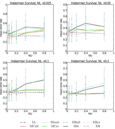
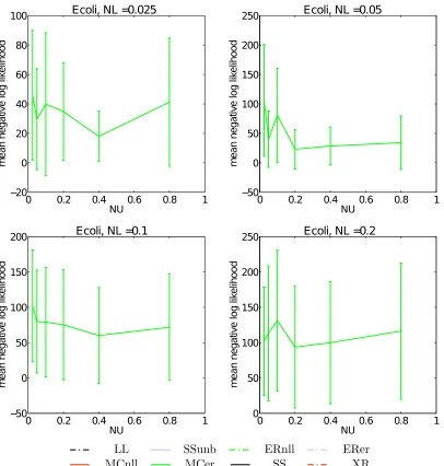
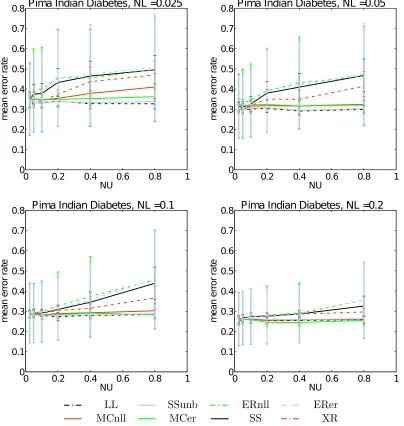
Figure 1 consists of four plots, showing how the mean negative log likelihood of the
Blood data set varies as NU is increased, for all four values of NL tested. Error bars indicate a single standard deviation. Note how for small values ofNU all methods perform similarly, with some benefit from using unlabelled data. As NU increases and the upper bound weakens, the methods begin to diverge - theER methods, along with SSband XR
worsen consistently. LL remains approximately constant (as expected) and slightly larger than SSunb. MCnll sits somewhere between LL and SSunb, worsening a little as the proportion of unlabelled data grows. This qualitative description of the observed behaviour applies to a significant proportion of the results. The main exceptions to this trend were in theGlass, Wineand Haber data sets for small values of NL, where competing methods (noticeably XR) performed better though this advantage tended to tail off as NL grew -for example see Figure 3, which shows the Haberman data set per-forming very well under
XR training.
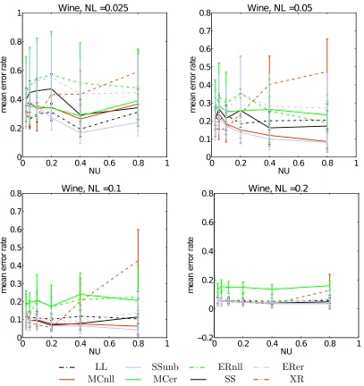
Figure 2 shows how the mean error rate of the same data set varies. For small quantities of labelled data SSunb tends to tie withLL. However as the quantity of labelled data grows competing methods begin to out perform it. In general we found that the proposed unbi-ased method was not always best (most commonly being out performed byXR), but often very competitive. It also rarely showed degradation in behaviour as the quantity of unla-belled data was increased - as we would expect, given the manner in which it automatically downgrades the influence of additional unlabelled samples.
0 0.2 0.4 0.6 0.8 1 0
2 4 6 8 10 12
NU
m
e
a
n
n
e
g
a
ti
v
e
lo
g
lik
e
lih
o
o
d
Blood Transfusion, NL =0.025
0 0.2 0.4 0.6 0.8 1
0 2 4 6 8 10
NU
m
e
a
n
n
e
g
a
ti
v
e
lo
g
lik
e
lih
o
o
d
Blood Transfusion, NL =0.05
0 0.2 0.4 0.6 0.8 1
0 1 2 3 4 5 6
NU
m
e
a
n
n
e
g
a
ti
v
e
lo
g
lik
e
lih
o
o
d
Blood Transfusion, NL =0.1
0 0.2 0.4 0.6 0.8 1
0.5 1 1.5 2 2.5 3 3.5 4 4.5
NU
m
e
a
n
n
e
g
a
ti
v
e
lo
g
lik
e
lih
o
o
d
Blood Transfusion, NL =0.2
LL SSunb ERnll ERer
MCnll MCer SSb XR
Figure 1: Four sample plots of the mean negative log likelihood of the Blood data set for a variety of values of NL, as NU grows. Note that M Cer is excluded, as it significantly underperformed and caused unfavourable axis scaling.
0 0.2 0.4 0.6 0.8 1 0
0.1 0.2 0.3 0.4 0.5 0.6 0.7 0.8
NU
m
e
a
n
e
rr
o
r
ra
te
Blood Transfusion, NL =0.025
0 0.2 0.4 0.6 0.8 1
0 0.1 0.2 0.3 0.4 0.5 0.6 0.7 0.8
NU
m
e
a
n
e
rr
o
r
ra
te
Blood Transfusion, NL =0.05
0 0.2 0.4 0.6 0.8 1
0 0.1 0.2 0.3 0.4 0.5 0.6 0.7 0.8
NU
m
e
a
n
e
rr
o
r
ra
te
Blood Transfusion, NL =0.1
0 0.2 0.4 0.6 0.8 1
0 0.1 0.2 0.3 0.4 0.5 0.6 0.7 0.8
NU
m
e
a
n
e
rr
o
r
ra
te
Blood Transfusion, NL =0.2
LL SSunb ERnll ERer
MCnll MCer SSb XR
Figure 2: Four sample plots of the mean error rate of the Blood data set for a variety of values ofNL, as NU grows.
better. What is also notable is how, while several other methods initially provide a bonus when NU is small (where the proportion rises above 0.5, indicating that they were more likely than not to improve learning), they tend to degrade quite rapidly as unlabelled data is added, often making it more probable that they will worsen performance by the time
0 0.2 0.4 0.6 0.8 1 0
0.2 0.4 0.6 0.8 1
NU
m
e
a
n
e
rr
o
r
ra
te
Haberman Survival, NL =0.025
0 0.2 0.4 0.6 0.8 1
0 0.1 0.2 0.3 0.4 0.5 0.6 0.7 0.8
NU
m
e
a
n
e
rr
o
r
ra
te
Haberman Survival, NL =0.05
0 0.2 0.4 0.6 0.8 1
0 0.1 0.2 0.3 0.4 0.5 0.6 0.7 0.8
NU
m
e
a
n
e
rr
o
r
ra
te
Haberman Survival, NL =0.1
0 0.2 0.4 0.6 0.8 1
0 0.1 0.2 0.3 0.4 0.5 0.6 0.7 0.8
NU
m
e
a
n
e
rr
o
r
ra
te
Haberman Survival, NL =0.2
LL SSunb ERnll ERer
MCnll MCer SSb XR
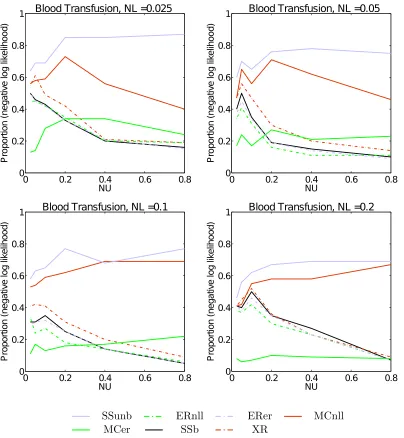
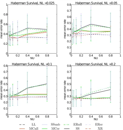
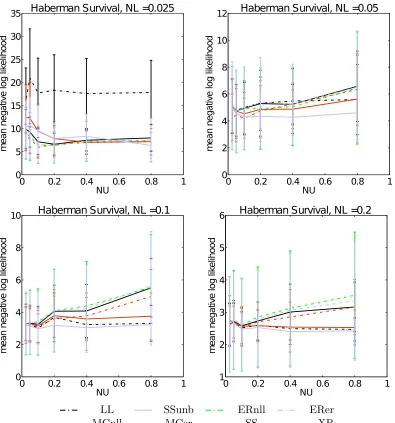
Figure 3: Four sample plots of the proportion of tests in which each semi-supervised learning scheme outperformed learning on the labelled data alone as measured by the negative log likelihood on theHabermandata set for a variety of values of NL, asNU grows.
0 0.2 0.4 0.6 0.8 0 0.2 0.4 0.6 0.8 1 NU P ro p o rt io n (n e g a ti v e lo g lik e lih o o d )
Blood Transfusion, NL =0.025
0 0.2 0.4 0.6 0.8
0 0.2 0.4 0.6 0.8 1 NU P ro p o rt io n (n e g a ti v e lo g lik e lih o o d )
Blood Transfusion, NL =0.05
0 0.2 0.4 0.6 0.8
0 0.2 0.4 0.6 0.8 1 NU P ro p o rt io n (n e g a ti v e lo g lik e lih o o d )
Blood Transfusion, NL =0.1
0 0.2 0.4 0.6 0.8
0 0.2 0.4 0.6 0.8 1 NU P ro p o rt io n (n e g a ti v e lo g lik e lih o o d )
Blood Transfusion, NL =0.2
SSunb ERnll ERer MCnll
MCer SSb XR
Figure 4: Four sample plots of the proportion of tests in which each semi-supervised learning scheme outperformed learning on the labelled data alone as measured by the negative log likelihood on the Blood data set for a variety of values of NL, as NU grows.
0 0.2 0.4 0.6 0.8 0
0.2 0.4 0.6 0.8 1
NU
P
ro
p
o
rt
io
n
(e
rr
o
r)
Blood Transfusion, NL =0.025
0 0.2 0.4 0.6 0.8
0 0.2 0.4 0.6 0.8 1
NU
P
ro
p
o
rt
io
n
(e
rr
o
r)
Blood Transfusion, NL =0.05
0 0.2 0.4 0.6 0.8
0 0.2 0.4 0.6 0.8 1
NU
P
ro
p
o
rt
io
n
(e
rr
o
r)
Blood Transfusion, NL =0.1
0 0.2 0.4 0.6 0.8
0 0.2 0.4 0.6 0.8 1
NU
P
ro
p
o
rt
io
n
(e
rr
o
r)
Blood Transfusion, NL =0.2
SSunb ERnll ERer MCnll
MCer SSb XR
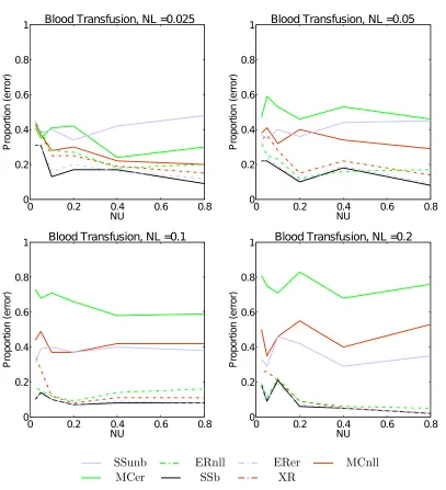
Figure 5: Four sample plots of the proportion of tests in which each semi-supervised learning scheme outperformed learning on the labelled data alone as measured by the error rate on theBlood data set for a variety of values ofNL, asNU grows.
6. Conclusions
Additionally, we have demonstrated a simple example of a new unbiased objective func-tion which approximately minimises KL(P(X, Y)||P(X, Y|θ)). This method is no more computationally complex than simply augmenting the likelihood, demonstrates very good behaviour with even very large quantities of unlabelled data, and requires quite weak condi-tions on the correlation between the conditional and generative components of the likelihood to reduce the variance of our estimator.
Although not covered, much of the analysis presented here likely to be applicable to regression problems as well as classification ones. We leave this as an avenue for possible future work.
Acknowledgments
This work was supported by the EPSRC.
Appendix A. Supplementary Results Of Unbiased Semi-Supervised Training
There are two measures of performance we examine, evaluated over a holdout set:
• The error rate
• The negative log likelihood
For each of these measures two statistics are calculated:
• The mean performance over all repetitions, and the associated variance.
• The proportion of repetitions in which the performance was better than that achieved using the labelled data alone.
The former gives an approximate measure of ‘average risk’, according to whether we consider risk in terms of misclassification rate (for example when designing a classification algorithm) or negative log likelihood (such as when building a compression algorithm, say). The latter tells us, for each measure of ‘risk’, whether or not including unlabelled data has improved or worsened our performance.
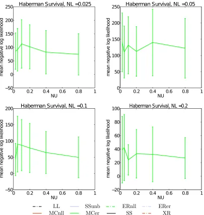
Multi conditional learning, when cross validated according to error rate, often gave extremely bad negative log likelihood results. This caused unfavourable scaling of the axis, making other results indistinguishable. As such, the mean negative log likelihood results of
MCerhave been separated out and plotted alone.
See the main body of the text for such as abbreviations and data sets.
A.1 Mean Errors And Negative Log Likelihood
0 0.2 0.4 0.6 0.8 1 0
0.1 0.2 0.3 0.4 0.5 0.6 0.7 0.8
NU
m
e
a
n
e
rr
o
r
ra
te
Diabetes, NL =0.025
0 0.2 0.4 0.6 0.8 1
0 0.1 0.2 0.3 0.4 0.5 0.6 0.7 0.8
NU
mean
error
rate
Diabetes, NL =0.05
0 0.2 0.4 0.6 0.8 1
0 0.1 0.2 0.3 0.4 0.5 0.6 0.7 0.8
NU
m
e
a
n
e
rr
o
r
ra
te
Diabetes, NL =0.1
0 0.2 0.4 0.6 0.8 1
0 0.1 0.2 0.3 0.4 0.5 0.6 0.7 0.8
NU
m
e
a
n
e
rr
o
r
ra
te
Diabetes, NL =0.2
LL SSunb ERnll ERer
MCnll MCer SS XR
Figure 6: Mean error results of Diabetes data set
A.2 Proportion In Which Performance Improves
0 0.2 0.4 0.6 0.8 1 2
4 6 8 10 12
NU
m
e
a
n
n
e
g
a
ti
v
e
lo
g
lik
e
lih
o
o
d
Diabetes, NL =0.025
0 0.2 0.4 0.6 0.8 1
1 2 3 4 5 6 7 8
NU
m
e
a
n
n
e
g
a
ti
v
e
lo
g
lik
e
lih
o
o
d
Diabetes, NL =0.05
0 0.2 0.4 0.6 0.8 1
1 2 3 4 5 6 7
NU
m
e
a
n
n
e
g
a
ti
v
e
lo
g
lik
e
lih
o
o
d
Diabetes, NL =0.1
0 0.2 0.4 0.6 0.8 1
1 1.5 2 2.5 3 3.5 4 4.5 5
NU
m
e
a
n
n
e
g
a
ti
v
e
lo
g
lik
e
lih
o
o
d
Diabetes, NL =0.2
LL SSunb ERnll ERer
MCnll MCer SS XR
0 0.2 0.4 0.6 0.8 1 50
100 150 200 250 300 350
NU
m
e
a
n
n
e
g
a
ti
v
e
lo
g
lik
e
lih
o
o
d
Diabetes, NL =0.025
0 0.2 0.4 0.6 0.8 1
50 100 150 200 250 300 350 400
NU
m
e
a
n
n
e
g
a
ti
v
e
lo
g
lik
e
lih
o
o
d
Diabetes, NL =0.05
0 0.2 0.4 0.6 0.8 1
0 50 100 150 200 250
NU
m
e
a
n
n
e
g
a
ti
v
e
lo
g
lik
e
lih
o
o
d
Diabetes, NL =0.1
0 0.2 0.4 0.6 0.8 1
−20 0 20 40 60 80 100 120 140
NU
m
e
a
n
n
e
g
a
ti
v
e
lo
g
lik
e
lih
o
o
d
Diabetes, NL =0.2
LL SSunb ERnll ERer
MCnll MCer SS XR
0 0.2 0.4 0.6 0.8 1 0
0.1 0.2 0.3 0.4 0.5 0.6 0.7 0.8
NU
m
e
a
n
e
rr
o
r
ra
te
SVMguide1, NL =0.025
0 0.2 0.4 0.6 0.8 1
0 0.1 0.2 0.3 0.4 0.5 0.6 0.7 0.8
NU
m
e
a
n
e
rr
o
r
ra
te
SVMguide1, NL =0.05
0 0.2 0.4 0.6 0.8 1
0 0.1 0.2 0.3 0.4 0.5 0.6 0.7 0.8
NU
m
e
a
n
e
rr
o
r
ra
te
SVMguide1, NL =0.1
0 0.2 0.4 0.6 0.8 1
0 0.1 0.2 0.3 0.4 0.5 0.6 0.7 0.8
NU
m
e
a
n
e
rr
o
r
ra
te
SVMguide1, NL =0.2
LL SSunb ERnll ERer
MCnll MCer SS XR
0 0.2 0.4 0.6 0.8 1 0
1 2 3 4 5 6 7
NU
m
e
a
n
n
e
g
a
ti
v
e
lo
g
lik
e
lih
o
o
d
SVMguide1, NL =0.025
0 0.2 0.4 0.6 0.8 1
0 1 2 3 4 5 6
NU
m
e
a
n
n
e
g
a
ti
v
e
lo
g
lik
e
lih
o
o
d
SVMguide1, NL =0.05
0 0.2 0.4 0.6 0.8 1
0 1 2 3 4 5
NU
m
e
a
n
n
e
g
a
ti
v
e
lo
g
lik
e
lih
o
o
d
SVMguide1, NL =0.1
0 0.2 0.4 0.6 0.8 1
0 0.5 1 1.5 2 2.5 3
NU
m
e
a
n
n
e
g
a
ti
v
e
lo
g
lik
e
lih
o
o
d
SVMguide1, NL =0.2
LL SSunb ERnll ERer
MCnll MCer SS XR
0 0.2 0.4 0.6 0.8 1 −100
0 100 200 300 400
NU
m
e
a
n
n
e
g
a
ti
v
e
lo
g
lik
e
lih
o
o
d
SVMguide1, NL =0.025
0 0.2 0.4 0.6 0.8 1
−50 0 50 100 150 200 250 300
NU
m
e
a
n
n
e
g
a
ti
v
e
lo
g
lik
e
lih
o
o
d
SVMguide1, NL =0.05
0 0.2 0.4 0.6 0.8 1
−50 0 50 100 150
NU
m
e
a
n
n
e
g
a
ti
v
e
lo
g
lik
e
lih
o
o
d
SVMguide1, NL =0.1
0 0.2 0.4 0.6 0.8 1
−40 −20 0 20 40 60 80 100 120
NU
m
e
a
n
n
e
g
a
ti
v
e
lo
g
lik
e
lih
o
o
d
SVMguide1, NL =0.2
LL SSunb ERnll ERer
MCnll MCer SS XR
0 0.2 0.4 0.6 0.8 1 0
0.2 0.4 0.6 0.8 1
NU
m
e
a
n
e
rr
o
r
ra
te
Wine, NL =0.025
0 0.2 0.4 0.6 0.8 1
0 0.1 0.2 0.3 0.4 0.5 0.6 0.7 0.8
NU
m
e
a
n
e
rr
o
r
ra
te
Wine, NL =0.05
0 0.2 0.4 0.6 0.8 1
0 0.1 0.2 0.3 0.4 0.5 0.6 0.7 0.8
NU
m
e
a
n
e
rr
o
r
ra
te
Wine, NL =0.1
0 0.2 0.4 0.6 0.8 1
−0.2 0 0.2 0.4 0.6 0.8
NU
m
e
a
n
e
rr
o
r
ra
te
Wine, NL =0.2
LL SSunb ERnll ERer
MCnll MCer SS XR
0 0.2 0.4 0.6 0.8 1 0
50 100 150 200
NU
m
e
a
n
n
e
g
a
ti
v
e
lo
g
lik
e
lih
o
o
d
Wine, NL =0.025
0 0.2 0.4 0.6 0.8 1
0 10 20 30 40 50 60 70 80
NU
m
e
a
n
n
e
g
a
ti
v
e
lo
g
lik
e
lih
o
o
d
Wine, NL =0.05
0 0.2 0.4 0.6 0.8 1
−10 0 10 20 30 40 50
NU
m
e
a
n
n
e
g
a
ti
v
e
lo
g
lik
e
lih
o
o
d
Wine, NL =0.1
0 0.2 0.4 0.6 0.8 1
0 2 4 6 8 10
NU
m
e
a
n
n
e
g
a
ti
v
e
lo
g
lik
e
lih
o
o
d
Wine, NL =0.2
LL SSunb ERnll ERer
MCnll MCer SS XR
0 0.2 0.4 0.6 0.8 1 20
30 40 50 60 70 80 90 100
NU
m
e
a
n
n
e
g
a
ti
v
e
lo
g
lik
e
lih
o
o
d
Wine, NL =0.025
0 0.2 0.4 0.6 0.8 1
20 30 40 50 60 70 80
NU
m
e
a
n
n
e
g
a
ti
v
e
lo
g
lik
e
lih
o
o
d
Wine, NL =0.05
0 0.2 0.4 0.6 0.8 1
20 40 60 80 100 120
NU
m
e
a
n
n
e
g
a
ti
v
e
lo
g
lik
e
lih
o
o
d
Wine, NL =0.1
0 0.2 0.4 0.6 0.8 1
20 40 60 80 100 120 140 160 180
NU
m
e
a
n
n
e
g
a
ti
v
e
lo
g
lik
e
lih
o
o
d
Wine, NL =0.2
LL SSunb ERnll ERer
MCnll MCer SS XR
0 0.2 0.4 0.6 0.8 1 0
0.2 0.4 0.6 0.8 1 1.2 1.4
NU
mean
error
rate
Glass Identification, NL =0.025
0 0.2 0.4 0.6 0.8 1
0 0.2 0.4 0.6 0.8 1
NU
m
e
a
n
e
rr
o
r
ra
te
Glass Identification, NL =0.05
0 0.2 0.4 0.6 0.8 1
0 0.2 0.4 0.6 0.8 1
NU
m
e
a
n
e
rr
o
r
ra
te
Glass Identification, NL =0.1
0 0.2 0.4 0.6 0.8 1
0 0.2 0.4 0.6 0.8 1
NU
m
e
a
n
e
rr
o
r
ra
te
Glass Identification, NL =0.2
LL SSunb ERnll ERer
MCnll MCer SS XR