The
fastclime
Package for Linear Programming and
Large-Scale Precision Matrix Estimation in
R
Haotian Pang [email protected]
Department of Electrical Engineering Princeton University
Olden St
Princeton, NJ 08540, USA
Han Liu [email protected]
Robert Vanderbei [email protected]
Department of Operations Research and Financial Engineering Princeton University
98 Charlton St
Princeton, NJ 08540, USA
Editor:Antti Honkela
Abstract
We develop an R package fastclime for solving a family of regularized linear program-ming (LP) problems. Our package efficiently implements the parametric simplex algorithm, which provides a scalable and sophisticated tool for solving large-scale linear programs. As an illustrative example, one use of our LP solver is to implement an important sparse pre-cision matrix estimation method calledCLIME(ConstrainedL1Minimization Estimator).
Compared with existing packages for this problem such asclimeandflare, our package has three advantages: (1) it efficiently calculates the full piecewise-linear regularization path; (2) it provides an accurate dual certificate as stopping criterion; (3) it is completely coded in C and is highly portable. This package is designed to be useful to statisticians and machine learning researchers for solving a wide range of problems.
Keywords: high dimensional data, sparse precision matrix, linear programming, para-metric simplex method, undirected graphical model
1. Introduction and Parametric Simplex Method
We introduce an R package, fastclime, that efficiently solves a family of regularized LP problems. Our package has two major components. First, we provide an interface function that implements the parametric simplex method (PSM). This algorithm can efficiently solve large-scale LPs. Second, we apply the PSM to implement an important sparse precision ma-trix estimation method called CLIME (Cai et al., 2011), which is useful in high-dimensional graphical models. In the rest of this section, we describe briefly the main idea of the PSM. We refer readers who are unfamiliar with simplex methods in general to Vanderbei (2008). Consider the LP problem
where A∈ Rn×d, c∈
Rd and b∈Rn are given and, “≥” and “≤” are defined component-wise. Simplex methods expect problems in “equality form”. Therefore, the first task is to introduce new variables which we tack onto the end ofβ and make it a longer vector ˆβ. We rewrite the constraints with the new variables on the left and the old ones on the right:
maxcTβN subject to: βB =b−AβN, βB≥0, βN ≥0.
Here,N ={1,2, . . . , d},B ={d+ 1, d+ 2, . . . , d+n}, andβBandβN denote subvectors of ˆβ associated with the indices in the set. In each iteration, one variable on the left is swapped with one on the right. In general, the variables on the left are called basic variables and the variables on the right are called nonbasic variables. As the algorithm progresses, the set of nonbasic variables changes and the objective function is re-expressed purely in terms of the current nonbasic variables and therefore the coefficients for the objective function change. In a similar manner, the coefficients in the linear equality constraints also change. We denote these changed quantities by ˆA, ˆb, and ˆc. Associated with each of these updated representations of the equations of the problem is a particular candidate “solution” obtained by setting βN = 0 and reading off the corresponding values for basic variables βB = ˆb. If ˆb≥0, then the candidate solution is feasible (that is, satisfies all constraints). If in addition ˆ
c≤0, then the solution is optimal.
Each variant of the simplex method is defined by the rule for choosing the pair of variables to swap at each iteration. The PSM’s rule is described as follows (Vanderbei, 2008). Before the algorithm starts, it parametrically perturbsb and c:
max(c+λc∗)Tβ subject to: Aβ≤b+λb∗, β≥0. (1)
Hereb∗ ≥0 andc∗ ≤0; they are calledperturbation vectors. With this choice, the perturbed problem is optimal for large λ. The method then uses pivots to systematically reduce λ
to smaller values while maintaining optimality as it goes. Once the interval of optimal λ
values covers zero, we simply set λ= 0 and read off the solution to the original problem. Sometimes there is a natural choice of the perturbation vectors b∗ and c∗ suggested by the underlying problem for which it is known that the initial solution to the perturbed problem is optimal for some value ofλ. Otherwise, the solver generates perturbations on its own.
If we are only interested in solving generic LPs, the PSM is comparable to any other variant of the simplex method. However, as we will see in the next section, the parametric simplex method is particularly well-suited to machine learning problems since the relaxation parameter λ in (1) is naturally related to the regularization parameter in sparse learning problems. This connection allows us to solve a full range of learning problems corresponding to all the regularization parameters. If a regularized learning problem can be formulated as (1), then the entire solution path can be obtained by solving one LP with the PSM. More precisely, at each iteration of the PSM, the current “solution” is the optimal solution for some interval ofλvalues. If these solutions are stored, then whenλreaches 0, we have the optimal solution to everyλ-perturbed problem for allλbetween 0 and the starting value.
2. Application to Sparse Precision Matrix Estimation
Estimating large covariance and precision matrices is a fundamental problem which has many applications in modern statistics and machine learning. We denote Ω = Σ−1, where Σ is the population covariance matrix. Under Gaussian model, the sparse precision ma-trix Ω encodes the conditional independence relationships among the variables and that is why sparse precision matrices are closely related to undirected graphs. Recently, sev-eral sparse precision matrix estimation methods have been proposed, including penalized maximum-likelihood estimation (MLE) (Banerjee et al., 2008; Friedman et al., 2007b,a, 2010), neighborhood selection method (Meinshausen and B¨uhlmann, 2006) and LP based methods (Cai et al., 2011; Yuan, 2011). In general, solvers based on penalized MLE meth-ods, such as QUIC (Hsieh et al., 2011) and HUGE (Zhao and Liu, 2012), are faster than the others. However, these MLE methods aim to find an approximate solution quickly whereas the linear programming methods are designed to find solutions that are correct essentially to machine precision. The comparison of classification performance can be found in Cai et al. (2011) and it is shown that CLIME uniformly outperforms the MLE methods. Be-cause of the good theoretical properties shown by CLIME, we would like to develop a fast algorithm for implementing this method which serves as an important building block for more sophisticated learning algorithms.
The CLIME solves the following optimization problem
minkΩk1 subject to: kΣnΩ−Idkmax≤λ and Ω∈Rd×d,
where Id is the d-dimensional identity matrix, Σn is the sample covariance matrix, and
λ > 0 is a tuning parameter. Here kΩk1 = Pj,k|Ω|j,k and k · kmax is the elementwise sup-norm. This minimization problem can be further decomposed intodsmaller problems, which allows us to recover the precision matrix in a column by column fashion. For thei-th subproblem, we get thei-th column of Ω, denoted as ˆβ, by solving
minkβk1 subject to: kΣnβ−eik∞≤λ and β ∈Rd, (2) wherekβk1=Pdj=1|βj|and ei ∈Rd is the i-th basis vector.
The originalclimepackage manually sets a default path forλand solves the LP problem for each different value ofλ. In this paper, we propose to use the PSM to solve this problem more efficiently. CLIME can be easily formulated in parametric simplex LP form. Let β+
and β− be the positive and negative parts of β. Sinceβ =β+−β− and kβk1 =β++β−, Equation (2) becomes:
minβ++β− subject to:
Σn −Σn
−Σn Σn
β+ β−
≤
λ+ei
λ−ei
. (3)
Comparing (1) and (3), we can give the following identification:
A=
Σn −Σn
−Σn Σn
, b=
ei
−ei
, c=
−1 .. . −1 , b
∗ = 1 .. . 1 , c
The path ofλdefined by the PSM corresponds to the path ofλas described in CLIME. Therefore, CLIME can be solved efficiently by the PSM; furthermore, when the optimal solution is sparse, the parametric simplex is able to find the optimal solution after very few iterations.
3. Performance Benchmark
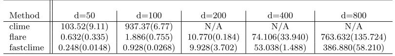
For our experiments we focused solely on CLIME. We compare the timing performance of our package with the packages flare and clime. Flare uses the Alternating Direction Method of Multipliers (ADMM) algorithm to evaluate CLIME (Li et al., 2012), whereas climesolves a sequence of LP problems for a certain specific set of values ofλ. As explained in Section 1, our method calculates the solution forallλ, whileflareandclimeuse a dis-crete set ofλvalues as specified in the function. We fix the sample sizento be 200 and vary the data dimension dfrom 50 to 800. We generate our data usingfastclime.generator, without any particular data structures. Clime and fastclime are based on algorithms that solve problems to machine precision (10−5). Flare, on the other hand, is an ADMM-based algorithm that stops when the change from one iteration to the next drops below the same threshold. As shown in Table 1, fastclime performances significantly faster than clime when d equals 50 and 100. When d becomes large, we are not able to obtain re-sults fromclime in one hour. We also notice that, in most cases,fastclimeperformances consistently better than flare, and it has a smaller deviation compared with flare. The reasonfastclimeoutperforms the other methods is primarily because the PSM only solves one LP problem to get the entire solution path for all λ quickly and without using much memory. The code is implemented on a i5-3320 2.6GHz computer with 8G RAM, and the R version used is 2.15.0.
Method d=50 d=100 d=200 d=400 d=800
clime 103.52(9.11) 937.37(6.77) N/A N/A N/A
flare 0.632(0.335) 1.886(0.755) 10.770(0.184) 74.106(33.940) 763.632(135.724) fastclime 0.248(0.0148) 0.928(0.0268) 9.928(3.702) 53.038(1.488) 386.880(58.210)
Table 1: Average Timing Performance of Three Solvers in Seconds
4. Summary and Acknowledgements
References
O. Banerjee, L. E. Ghaoui, and A. d’Aspremont. Model selection through sparse maximum likelihood estimation. Journal of Machine Learning Research, 9:485–516, 2008.
T. Cai, W. Liu, and X. Luo. A constrained l1 minimization approach to sparse precision matrix estimation. J. American Statistical Association, 106:594–607, 2011.
J. Friedman, T. Hastie, H. H¨ofling, and R. Tibshirani. Pathwise coordinate optimization. Annals of Applied Statistics, 1(2):302–332, 2007a.
J. Friedman, T. Hastie, and R. Tibshirani. Sparse inverse covariance estimation with the graphical lasso. Biostatistics, 9(3):432–441, 2007b.
J. Friedman, T. Hastie, and R. Tibshirani. Regularization paths for generalized linear models via coordinate descent. Journal of Statistical Software, 33(1), 2010.
C-J. Hsieh, M. A. Sustik, I. S. Dhillon, and P. Ravikumar. Sparse inverse covariance matrix estimation using quadratic approximation. Advances in Neural Information Processing Systems, 24, 2011.
X. Li, T. Zhao, X. Yuan, and H. Liu. An R package flare for high dimensional linear regression and precision matrix estimator. R Package Vigette, 2012.
N. Meinshausen and P. B¨uhlmann. High dimensional graphs and variable selection with the lasso. Annals of Statistics, 34(3):1436–1462, 2006.
R. Vanderbei. Linear Programming, Fundations and Extensions. Springer, 2008.
M. Yuan. High dimensional inverse covariance matrix estimation via linear programming. Journal of Machine Learning Research, 11:2261–2286, 2011.