Learning Using Anti-Training with Sacrificial Data
Michael L. Valenzuela [email protected]
Jerzy W. Rozenblit [email protected]
Electrical and Computer Engineering Department University of Arizona
1230 E. Speedway Blvd.
Tucson, AZ 85721, UNITED STATES
Editor:Martin Pelikan
Abstract
Traditionally the machine-learning community has viewed the No Free Lunch (NFL) theorems for search and optimization as a limitation. We review, analyze, and unify the NFL theorem with the perspectives of ``blind"" search and meta-learning to arrive at necessary conditions for improving black-box optimization. We survey meta-learning literature to determine when and how meta-learning can benefit machine learning. Then, we generalize meta-learning in the context of the NFL theorems, to arrive at a novel technique called anti-training with sacrificial data (ATSD). Our technique applies at the meta level to arrive at domain specific algorithms. We also show how to generate sacrificial data. An extensive case study is presented along with simulated annealing results to demonstrate the efficacy of the ATSD method.
Keywords: Machine Learning, Optimization, Meta Optimization, No Free Lunch, Anti-Training, Sacrificial Data
1. Introduction
Most types of machine learning involve fitting a model to data. These models may be
artificial neural networks, Bayesian networks, cluster centers, decision trees, etc. The
fitting process uses objective/fitness functions to determine how well the learned model
represents the training data. While many models (e.g., artificial neural networks) have
training algorithms (e.g., backpropagation), it is not always clear which algorithm is best
to use for a particular data set. This is the issue John Rice describes as the algorithm selection problem (Rice, 1976).
The same virtue that makes black-box optimizers so widely used is also their inherent weakness---black-box optimizers use only a history of inputs into, and outputs from an objective function. This allows black-box optimizers to function on symbolic representa-tions, experimental data, or results from simulations. The black-box optimizer does not use any knowledge about the symbolic function, data, or simulation. The No Free Lunch (NFL) theorems for search and optimization state that any such black-box optimization is expected to perform on average as well as a random guesser (Wolpert and Macready, 1997). If the objective function comes from a slow simulation or a physical experiment, then every function evaluation is precious. Thus, an algorithm tailored toward a particular problem distribution can make better use of the function evaluations.
In this work, we introduce a completely novel concept: anti-training with sacrificial
data, for tailoring learning and optimization algorithms to problem distributions. At its
base, anti-training is a generalization of a type of meta-learning. We take advantage of the fact that all optimization algorithms perform the same on average (according to the NFL theorems). Essentially, anti-training worsens the performance over problems suspected to be impossible or exceedingly unlikely to occur. Since the average performance remains constant, the performance elsewhere must increase. Consider the following water balloon analogy: the NFL theorems function as the conservation of volume. Squeezing the water (performance) out of one area of the balloon will transfer it to other areas.
Unlike many forms of meta-learning, anti-training inherently adheres to the NFL the-orems since it is derived through the manipulation of the NFL thethe-orems. Anti-training is expected to benefit learning performance whenever the objective functions are compressible. Moreover, because the sacrificial data used by anti-training is inexpensive to generate, it is possible to use anti-training where meta-learning cannot be applied. It can also be applied in conjunction with meta-learning and can prevent overtraining.
Following preliminaries and nomenclature in Section 2, we rewrite an NFL theorem to derive our technique and proceed to analyze it in Section 3. Section 4 discusses how to generate the sacrificial data required for anti-training. We extensively discuss several experiments in Section 5 and the results in Section 6. We then conclude with a discussion and future work in Section 7.
2. Preliminaries and Background
The original NFL theorems apply to arbitrarily large finite domains (e.g., combinatorial
optimization problems). Wolpert and Macready (1997) argue that this makes sense since
computers only have a finite number of bits; the search space \scrX and output space\scrY are
typically bit sequences. Continuing with their notation, letf be a function representing an
optimization problem (e.g., error function, distance, etc.) and\scrF be the set of all functions
having an input x\in \scrX and an output y \in \scrY . If | \scrX | is the size of the search space and | \scrY |
is the size of the output space, then the size of the function space is | \scrF | =| \scrY | | \scrX | (Wolpert
and Macready, 1997). (Just to realize the order of magnitude of | \scrF | , consider a function
with a 16-bit input and an 8-bit output; then | \scrF | = 2219 \approx 2.6\cdot 10157826. This is a large
number of possible functions, but it is still finite.) Moreover, let
\bullet P(f) be a probability mass function, describing the probability off occurring,
\bullet P\^(f) be an estimate ofP(f),
\bullet abe a black-box algorithm that samplesf and uses the input-output data to generate
the next input into f,
\bullet m\in \{ 1, . . . ,| \scrX | \} be the number of unique inputs,
\bullet dx
m be a set of the firstm unique inputs,1
\bullet dym be a set of the corresponding outputs,
\bullet dm be shorthand for dym anddxm combined,
\bullet P\bigl(
dym| f, m, a\bigr) be the conditional probability of finding dym given an algorithm a
iteratedm times on a fitness functionf, and
\bullet \Phi \bigl( dym
\bigr)
be a function that converts the output to some performance metric.
For brevity, we provide the following terms:
\bullet anti-training with sacrificial data is shortened toATSD,
\bullet anti-training with sacrificial data combined with meta-learning is abbreviated as
ATSD+ML,
\bullet meta-learning is abbreviated as ML, and
\bullet No Free Lunch to be abbreviated asNFL.
2.1 NFL
Briefly, the NFL theorems state that for both static and time-varying optimization problems, all algorithms perform the same when averaged across all problems (Wolpert and Macready, 1997). We will focus on static problems. The NFL theorems are cast in a probabilistic framework:
Theorem 1
\sum
f\in \scrF
P\bigl( dym| f, m, a1
\bigr)
= \sum
f\in \scrF
P\bigl( dym| f, m, a2
\bigr)
. (1)
In the words of the authors: ``this means in particular that if some algorithm's per-formance is superior to that of another algorithm over some set of optimization problems, then the reverse must be true over the set of all other optimization problems."" The above
equation is true regardless of the problem distribution, P(f). This is different from saying
all algorithms are equal. For all algorithms to be equal we require:
Theorem 2
\sum
f\in \scrF
P(f)P\bigl( dym| f, m, a1
\bigr)
= \sum
f\in \scrF
P(f)P\bigl( dym| f, m, a2
\bigr)
. (2)
This explicitly depends on P(f). Following the proof provided in Wolpert and Macready
(1997), (2) requires
\sum
f\in \scrF
P(f)P\bigl(
dy1| f, m= 1, a\bigr)
=\sum
f\in \scrF
P(f)\delta \Bigl( dy1, f\bigl(
dx1\bigr) \Bigr)
(3)
to be independent of dx1 and hence a. This sum is used in the base case for the inductive
proof in Wolpert and Macready (1997), where for information theoretic reasons, they assume
a P(f) to be uniform. P(f) could also be any distribution following \prod
x\in \scrX P(y = f(x)),
or certain distributions with specific correlations between costs and inputs (Wolpert and Macready, 1997).
The NFL theorems have been extended to include additional priors and results. Schu-macher et al. (2001) extend this to include sets of functions closed under permutations of the input-space. Thus, all algorithms sum to the same performance and generate the same
collection ofdmwhen all functions are considered (Schumacher et al., 2001). Other analyses
and extensions can be found in Culberson (1998); Droste et al. (2002); Corne and Knowles (2003a,b); Igel and Toussaint (2003, 2004); Giraud-Carrier and Provost (2005); Whitley and Watson (2005); Wolpert and Macready (2005); Auger and Teytaud (2007, 2010)). The results of these studies show that the No Free Lunch theorems are valid, but their relevance varies depending on the situation. Yet, despite all the extensions and debate, ``there are no specific methods or algorithms that directly follow from NFL"" (Whitley and Watson, 2005). In the paper, we provide a method that stems from the NFL theorems.
The NFL theorems treat the definition of ``algorithms"" differently than the typical definition of algorithm implies. In the NFL theorems, the ``algorithms"" are more about exploring the search space (points) in some order than about the actual instructions carried out by the computer. Two ``algorithms"" are considered identical if they always visit points in the same order, even if the underlying programming code is different. Likewise, the NFL theorems call two ``algorithms"" different even if they share the same code, but run with
different hyper-parameters (e.g.,step-size, branching preference, etc.) so long as points are
visited in a different order.
In the following subsections, we briefly summarize information theory and meta-learning prerequisites needed to establish the foundations for ATSD.
2.2 Information Theory
Information theory is a useful tool for studying learning (Bialek et al., 2001; Rissanen, 1984, 1986, 1987, 1989) and analyzing the NFL theory (Schumacher et al., 2001). In informa-tion theory, there are two common measures of complexity: ``entropy"" and ``Kolmogorov complexity."" Entropy is typically defined as:
H(X) =\sum
x\in \scrX
where X is a discrete random variable and \scrX is the support of X. Entropy is sometimes interpreted as random variable's uncertainty. Kolmogorov complexity, sometimes called al-gorithmic entropy or complexity under analysis, cannot be specified so concisely. Essentially Kolmogorov complexity describes the size of the smallest program needed to reproduce a
specified sequence (e.g.,bits, characters, numbers, etc.). Since there are multiple languages
and machine architectures, Kolmogorov complexity is an incomputable function (Cover and
Thomas, 2006; Li and Vit\'anyi, 2008). In this paper, when we say something is compressible
or incompressible, we mean this in the sense of Kolmogorov complexity. Information
theory shows most functions are incompressible (a proof can be found in the work of Cover and Thomas (2006)). One should be careful to distinguish the ideas of a function being compressible versus being represented in polynomial space. If the number of bits needed to represent a sequence can be halved, there are still an exponential number of such bit sequences.
Culberson (1998) indirectly uses entropy when discussing the NFL theorems from dif-ferent degrees of ``blindness."" The degrees of ``blindness"" range from complete information (the objective function is known) to no information. When these degrees of ``blindness"" are recast in a probabilistic framework, one can see that the random variable describing the objective function has zero entropy in the case of complete information and maximal entropy when nothing is known. Thus a main point of Culberson (1998) is that optimization performance degrades as the problem distribution becomes more complex.
2.3 Meta-learning
Before we begin our formulation of ATSD, due to the strong ties between ML and ATSD, it is important to address questions pertaining to the NFL theorems and ML. The first and probably most important question is: ``can ML successfully improve performance in light of the NFL theorems?"" If so, when does ML help? How can one judge the quality of an algorithm's learning biases?
ML is generally concerned with learning to learn better. Nevertheless, it can be
applied to learning to optimize better. One perspective of ML is the algorithm selection problem (Rice, 1976). That is, given a specific instance of a problem, which algorithm solves the problem best? Giraud-Carrier and Provost (2005) address whether ML can escape the limitations imposed by the NFL theorems. Their ultimate conclusion is that only techniques
that learn about the problem distribution P(f) can overcome the NFL theorems. Hence,
ML can be useful in light of the NFL theorems.
Vilalta and Drissi (2002) introduce two important ML concepts. One is that of struc-tured versus random problems. Strucstruc-tured problems have lower Kolmogorov complexity
than random problems. This structure can be exploited by algorithms to solve these
problems more efficiently. By this definition, random problems have no such structure that ML can exploit. Consequently, ML is limited (with respect to its effectiveness) to structured problems. In terms of entropy, structured problems may still require exponential space to
represent. To see this let there be| \scrF | functions represented by 2nbits, then there are about
with the size of | \scrF | . In other words, ML applies as long as most problems are considered irrelevant.
One may like to know how to measure one's success in selecting an algorithm. To do so, we first need a definition of success. Vilalta and Drissi (2002) introduce the concept of
algorithm biases expressed as restrictions and rankings of potential hypotheses (the truef).
In our formal notation, this means each algorithm assumes some P(f). Then successfully
selecting an algorithm means that the selected algorithm's assumed problem distribution matches the actual problem distribution. Both a theoretical and realistic measure exist to judge how well these match. Wolpert and Macready (1997) propose using the inner product
betweenP(f) and P(dym| f, m, a) overf \in \scrF for a desireddym. However, this method is only
theoretical as computing the inner product is difficult due to the size of \scrF . A much more
realistic measure is the off-training-set error (Wolpert, 2001).
We can use the answers to these three questions to lead us down a path of investigation. When ML samples from the problem distribution, the distributions are compressible (most problems are irrelevant), and the current method is suboptimal, then ML may operate within the NFL framework. Therefore, we will investigate how ML may manifest itself in the NFL framework. Second, due to the similarities between ML and ATSD, we will derive ATSD by applying an opposite goal to the opposite data. This in effect forms a ``dual problem,"" which leads to our formulation of ATSD.
3. Anti-training
Section 2.3 gives us a research direction: derive ML from the NFL theorems, and subse-quently, ATSD from that. To ensure our technique follows from (1), we begin by rewriting
one side. First, we split\scrF into three partitions (non-overlapping sets that cover the whole
set):
\sum
f\in \scrF
P\bigl( dym| f, m, a\bigr) =\sum
f\in \scrF +
P\bigl( dym| f, m, a\bigr) +\sum
f\in \scrF 0
P\bigl( dym| f, m, a\bigr) +\sum
f\in \scrF -
P\bigl( dym| f, m, a\bigr) . (4)
Here \scrF +, is the partition of problems already encountered, considered likely, or relevant;
\scrF - represents the partition of problems that cannot occur (in the given context) or are
considered unlikely to occur; and \scrF 0 consists of problems that are borderline likely or
undefined. Equation 4 explicitly shows that we can trade-off performance between problem
sets. Performance gained overf \in \scrF + must be lost over f \in \scrF 0\cup \scrF - .
The inquisitive reader may wonder why we use three partitions and particularly why we
include the\scrF 0 partition. We include\scrF 0 for three reasons: first, an objective function does
not always cleanly lie in either \scrF + or \scrF - . This is because we avoid strict mathematical
definitions of\scrF +,\scrF 0, and \scrF - . One may choose, for example, \scrF + =\{ f| P(f)>100/| \scrF | \} and
\scrF - =\{ f| P(f)<0.01/| \scrF | \} . This flexibility necessitates\scrF 0. Second,\scrF 0is useful for describing
an important difference between ML and ATSD: the difference between the forthcoming (6)
and (7). Third, when approximating\scrF + and\scrF - ,\scrF 0 is a catch-all for the remaining cases.
Thus, three partitions are the minimum number needed to capture these degrees of freedom.
Equation 1 implies (4) is independent of a. However, each sum over a partition of
sets of functions not closed under permutation.2 Schumacher et al. (2001) show in their Lemmas 1 and 2 that the NFL theorems apply if and only if the set of functions is closed
under permutation. Since the fraction of sets closed under permutation is exceedingly
rare (Igel and Toussaint, 2003), the NFL theorems fail to apply, with high probability, to
each partitioning of \scrF . In turn, this means that each sum is generally allowed to change,
implying that it is possible to improve the performance over \scrF +.
Let us extend (4) in two ways. First, multiply by \Phi \bigl( dym
\bigr)
(a performance metric such as
final error) and bring it inside the sum. Second, sum several \sum
f\in \scrF \Phi \bigl(
dym
\bigr)
P\bigl(
dym| f, m, a
\bigr)
together for different values of dym. Then we have
\sum
dym \sum
f\in \scrF
u=\sum
dym \left(
\sum
f\in \scrF +
u+ \sum
f\in \scrF 0
u+ \sum
f\in \scrF -
u
\right)
, (5)
where
u= \Phi \bigl( dym\bigr) P\bigl( dym| f, m, a\bigr) .
3.1 Anti-training as Meta-learning
Recall that a type of ML taking into account the NFL theorems is the one that attempts
to learnP(f) directly (Giraud-Carrier and Provost, 2005). However, this is often infeasible
due to the cardinality of \scrF . A simple alternative to approximate this method is to
learn an optimizer that performs well on the empirically common functions. This is a
meta-optimization problem to improve the performance over \scrF +. More accurately, the
meta-optimization will improve the conditional expected value of \Phi \bigl( dym
\bigr)
. Without loss of
generality, hence forth assume \Phi is a performance metric to be minimized (e.g., an error
function). Then, improving (minimizing) the conditional expected value means:
a \star = arg min
a
\sum
dym \sum
f\in \scrF +
\Phi \bigl(
dym\bigr) \^
P+(f)P
\bigl(
dym| f, m, a\bigr)
.
However, the above equation is neither governed by nor does it follow from the NFL
theorems! The introduction of a function dependent on f, in this case the approximation
\^
P+(f), generally voids the NFL requirement that (3) is independent of a. Nevertheless,
if we consider the typical approximation of \^P+(f) used in practice, we realize that rarely
does an identical objective function occur twice. See Appendix A for further justification
of this assertion. This means \^P+(f) is practically going to be a two-valued function: 0 and
\bigm| \bigm|
\bigm| P\^+(f)
\bigm| \bigm| \bigm|
- 1
. Thus, in practice we drop the term \^P+(f). This recovers the first term on the
right-hand-side of (5), which follows from the NFL theorems:
a \star = arg min
a
\sum
dym \sum
f\in \scrF +
\Phi \bigl(
dym\bigr)
P\bigl(
dym| f, m, a\bigr)
. (6)
We make several more notes about the above equation. First, when using a deterministic
a (or a random algorithm with a fixed random seed) P\bigl( dym| f, m, a
\bigr)
will be either 0 or 1;
only a single dym will be produced. This makes it easier to optimize in practice. Second,
\Phi \bigl(
dym
\bigr)
determines the behavior of a \star ; a \star could produce a low final error, low cumulative
error, etc. While it is also possible to modify (6) to optimize over the cross-validation error, care must be taken as cross-validation alone is subject to the NFL theorem (Wolpert, 2001).
Typically\scrF + will be approximated using samples from a problem distributionP(f) arising
from a limited domain. Additionally, (6) says nothing about the search for a \star . Unless a
is being modified intelligently, the meta-optimization problem will be subject to the NFL theorems itself. This means that finding better algorithms will be possible, but costly.
The NFL theorems say that any performance gained over a set of functions must be lost over the set's complement. Equation 4 must remain constant. Thus, ML improves
the performance over \scrF + at the cost of performance over \scrF 0 \cup \scrF - . This is potentially
detrimental for prediction, generalization, and avoiding overfitting. To help mitigate this
issue we now introduce anti-training with sacrificial data (ATSD). This means ATSD is
about the optimization of one of the terms from (5):
a \star = arg max
a
\sum
dym \sum
f\in \scrF -
\Phi \bigl( dym\bigr) P\bigl( dym| f, m, a\bigr) . (7)
This translates into
a \star = arg min
a
\sum
dym \sum
f\in \scrF 0\cup \scrF +
\Phi \bigl( dym\bigr) P\bigl( dym| f, m, a\bigr) .
Again, without loss of generality, we treat \Phi as an error function to be minimized. As one can see, ATSD is an approximate dual of ML. ATSD achieves an improvement in the
sum of performance over \scrF +\cup \scrF 0 by directly worsening the performance over \scrF - . If the
performance over \scrF - decreases, then by (4), the sum over \scrF 0\cup \scrF + must improve. Despite
ATSD being less efficient than ML, it has other benefits. For a more complete discussion, please see Sections 3.2 and 3.3.
It is critical to note that the performance improvement is over \scrF 0\cup \scrF +. Without
addi-tional care, ATSD could drop the performance over \scrF +, but improve the performance over
\scrF 0. To help avoid this, ATSD should be combined with ML (ATSD+ML). Combining (6)
and (7), we have
a \star = arg min
a
\sum
dym \left(
\sum
f\in \scrF +
\Phi \bigl( dym\bigr) P\bigl( dym| f, m, a\bigr) - \beta \sum
f\in \scrF -
\Phi \bigl( dym\bigr) P\bigl( dym| f, m, a\bigr)
\right)
(8)
where \beta \geq 0 determines the relative strength of anti-training. The above optimization
technique is just one straightforward approach to combining ML and ATSD. ATSD+ML can be achieved by using a meta-optimization technique similar to the aforementioned
process for ML. According to Bergstra and Bengio (2012), a random search for a \star is in
some sense optimal. Although, preliminary tests suggest that local searches find locally optimal continuous hyper-parameters on continuous domains.
We feel it is important to note that ATSD+ML is not strictly limited to operating over \sum
f\in \scrF + and
\sum
to simply using (8) with an adjusted \beta . The median is another statistic that could be used. Meta-optimizing using the medians would be the same as dynamically selecting one
or two f to improve or worsen their performance. For the same reason, percentiles are
valid statistics to improve or degrade. Since percentiles could be used, one may wonder if the interquartile-range (IQR) is a valid statistic for ATSD+ML. ATSD+ML should avoid
using the IQR statistic over\scrF - , as this amounts to improving the performance over some
f \in \scrF - .
Algorithm 1 demonstrates the basic approach. The parameter metaSearch is a search
algorithm for finding black-box search/optimization/learning algorithms; metaM etric is
Algorithm 1 Anti-Training Combined with Meta-Learning
1: Procedure Anti-Meta-Search(
metaSearch, metaM etric, pM etric, \scrF \^+, \scrF \^ - , m)
2: metaOut\leftarrow empty
3: repeat
4: searchAlg\leftarrow metaSearch(metaOut)
5: listP osP erf s\leftarrow empty
6: for allobjF unc\in \scrF \^+ do
7: optResults\leftarrow Optimize(searchAlg, pM etric, objF unc, m)
8: AppendoptResults\rightarrow listP osP erf s \{ Accumulate results from \^\scrF +\}
9: end for
10: listN egP erf s\leftarrow empty
11: for allobjF unc\in \scrF \^ - do
12: optResults\leftarrow Optimize(searchAlg, pM etric, objF unc, m)
13: AppendoptResults\rightarrow listN egP erf s \{ Accumulate results from \^\scrF - \}
14: end for
15: algP erf ormance\leftarrow metaMetric (listP osP erf s, listN egP erf s) \{ e.g., (8)\}
16: Append (searchAlg, algP erf ormance)\rightarrow metaOut
17: untilalgP erf ormanceis good enough
18: Return Argmin(metaOut)
1: Procedure Optimize(searchAlg, perf ormanceM etric, objF unc, m)
2: dm \leftarrow empty
3: foritr= 1 to itr=m do
4: x\leftarrow searchAlg(dm)
5: Append (x)\rightarrow dxm
6: y\leftarrow objF unc(dxm)
7: Append (y)\rightarrow dym
8: Append (dxm, dym)\rightarrow dm
9: perf ormance\leftarrow perf ormanceM etric(dm)
10: end for\{ Alternatively end when performance is good enough\}
11: return perf ormance \{ If ending when performance is good enough return number of
the metric for preferring one black-box algorithm over another, such as (8); and pM etric
is \Phi \bigl( dym
\bigr)
, which rates the quality of outputs. The subroutine Optimize is a black-box
search/optimization algorithm that runs the searchAlg to generate the inputdxm into the
black-box objective function objF unc.
Algorithm 1 starts by selecting, generating, or modifying a search/optimization/learning
algorithm. For simplicity, let us assume the goal is optimization. The optimization
subroutine generates the next inputxfrom the history of inputs and outputs. The objective
function (from \^\scrF - or \^\scrF +) is evaluated at x. This process is repeated, building up thedm
vector. After enough iterations, the subroutine returns the performance metric, \Phi \bigl(
dym\bigr) .
The performance over each f \in \scrF \^+ \cup \scrF \^ - is computed and stored using this subroutine.
The meta-fitness function evaluates the optimization algorithm using ATSD+ML. This whole process is repeated for enough iterations or until the algorithm's performance is good enough.
3.2 Analysis
We now present how effective the ATSD is from a theoretical perspective. An extensive, empirical study follows in Section 5. It is difficult to analyze ATSD without making strong assumptions. Thus, we make the following assumptions as general as possible and defend them using logic similar to that used in the original NFL theorems (Wolpert and Macready, 1997).
Allow an algorithm to be represented by its learning biases as discussed by Vilalta and
Drissi (2002). We choose to interpret these biases as ana priori rank ordering of functions.
To help illustrate this point, imagine an algorithm represented by a deck of cards, where each
card represents an objective functionf to be optimized. Denote Ra(f)\in
\bigl\{
1,2, . . . ,| \scrF | \bigr\} as
algorithma's ranking (i.e., position in the deck) off. A lower ranking means the algorithm
is more biased toward finding the optimal solution in fewer iterations. The function with
rank one will have its optimum input guessed first. Then allf \in \scrF in violation of the first
input-output pair,d1, are removed from the deck of hypotheses and the process is repeated.
Allow \^\scrF + and \^\scrF - to be samples from \scrF + and \scrF - respectively. Furthermore, since we
are working with domain specific optimizers, we may assume the majority of problems are not highly relevant:
\bigm| \bigm| \scrF +
\bigm|
\bigm| \ll | \scrF 0| \bigm|
\bigm| \scrF + \bigm| \bigm| \ll
\bigm| \bigm| \scrF -
\bigm| \bigm| .
Rather than debate the percentf \in \scrF - , allow
| \scrF | =c\bigm| \bigm| \scrF - \bigm| \bigm| ,
for a constantc. For example, if\bigm| \bigm| \scrF - \bigm|
\bigm| \approx | \scrF 0| thenc\approx 2.0. Nevertheless, we will continue to
usec symbolically to remain more flexible and general, allowing the reader to impose their
own assumptions.
f \in \scrF \^+lowers in rank, then on average allow allg\in \scrF + to lower proportionally by a factor
of\rho +.3 This will provide the average behavior for describing why ML works. To capture the
corresponding effects of ATSD, when somef\prime \in \scrF \^ - rises in rank due to meta-optimization,
allow all g\prime \in \scrF - to rise proportionally by a factor of \rho - . We use the symbols g and g\prime to
denote objective functions that are ``dragged"" along due to correlations in rankings. The
two factors, \rho + and \rho - , are functions of the compressibility of \^\scrF + and \^\scrF - respectively.
Assume that the meta-optimization task improves/degrades the rankings bypc(percent
change). That is, for f \in \scrF \^+ and f \in \scrF \^ - the ranking changes fromRa(f) to
Ra(f) (1 - pc) +pc, and
| \scrF | pc+Ra(f) (1 - pc)
respectively. Thus the differences in rank after ML and subsequently ATSD are approxi-mately
\bigl(
Ra(f) - 1
\bigr)
pc, and
\bigl(
| \scrF | - Ra(f)
\bigr)
pc.
If we assume the starting algorithm is chosen at random, then we can assume the
rankings are uniformly distributed: P(Ra(f)) \sim U
\bigl( 1,| \scrF | \bigr)
. This follows from the same
reasoning Wolpert and Macready (1997) use to argue thatP(f) ought to assume a uniform
distribution when lacking further information. Then
E\bigl[
Ra(f)
\bigr]
= | \scrF | + 1 2
Now, we will proceed to show that the expected rank improvements from ML and ATSD
are comparable. After accounting for rank correlations, improving a singlef \in \scrF \^+produces
on average
\mu +(f) =pc
\left(
Ra(f) - 1 -
\bigl(
Ra(f) - 1
\bigr)
\rho +
\sum
g\in \scrF +
\bigl(
Ra(g) - 1
\bigr)
\rho +
\right)
rank improvements. The term \bigl( Ra(f) - 1
\bigr)
\rho + is subtracted to avoid double counting f as
f \in \scrF +, and the term Ra(g)| g\in \scrF + is any function that may have its rank improved due
to correlations between problems. Substituting in the expected values of Ra(f) and Ra(g)
produces
E\bigl[ \mu +(f)
\bigr]
=pc
\Biggl(
| \scrF | - 1 2
\bigl( 1 - \rho +
\bigr)
+| \scrF | - 1 2
\bigm| \bigm| \scrF +
\bigm| \bigm| \rho +
\Biggr)
=pc
\Biggl(
| \scrF | - 1 2
\Biggr) \biggl(
1 + \Bigl(
\bigm| \bigm| \scrF +
\bigm|
\bigm| - 1
\Bigr)
\rho +
\biggr)
. (9)
Next we will compute the number of ranks degraded during ATSD. After accounting for
correlations, but being careful to avoid double counting f\prime , the number of ranks degraded
on average for anti-training a single f\prime \in \scrF \^ - is
\mu - \Bigl(
f\prime \Bigr) =pc
\left( \biggl(
| \scrF | - Ra
\Bigl(
f\prime \Bigr)
\biggr) \bigl(
1 - \rho - \bigr) + \sum
g\prime \in \scrF
- \biggl(
| \scrF | - Ra
\Bigl(
g\prime \Bigr)
\biggr)
\rho - \right)
.
Substituting in the expected values of Ra(f\prime ) andRa(g\prime ) produces
E
\biggl[
\mu - \Bigl(
f\prime \Bigr)
\biggr]
=pc
\Biggl(
| \scrF | - 1 2
\Biggr) \biggl(
1 +\Bigl( \bigm| \bigm| \scrF - \bigm|
\bigm| - 1
\Bigr)
\rho - \biggr)
. (10)
We cannot directly compare (9) and (10) yet. Equation 10 is in terms of ranks degraded
for f\prime \in \scrF - , not ranks improved for f \in \scrF +. We can calculate the expected number of
f \in \scrF + promotions as a result of anti-training demotions by multiplying (10) by the ratio
\bigm| \bigm| \scrF +
\bigm|
\bigm| /| \scrF | . Recalling | \scrF | =c
\bigm| \bigm| \scrF -
\bigm|
\bigm| , we have
E
\Bigl[
\mu \prime - (f) \Bigr]
=pc
\Biggl(
| \scrF | - 1 2
\Biggr) \left(
\zeta + \Biggl( \bigm|
\bigm| \scrF + \bigm| \bigm|
c - \zeta
\Biggr)
\rho - \right)
where\zeta = | \scrF +|
c| \scrF - | . Thus the relative power of ATSD versus ML is given by
E\Bigl[ \mu \prime - (f)\Bigr]
E\bigl[
\mu +(f)
\bigr] =
\Biggl(
\zeta + \biggl(
| \scrF +| c - \zeta
\biggr)
\rho - \Biggr)
\biggl(
1 +\Bigl( \bigm| \bigm| \scrF + \bigm|
\bigm| - 1
\Bigr)
\rho +
\biggr) . (11)
Note \zeta = | \scrF | \scrF | +| \approx 0 by assumption. Provided a sufficiently large \bigm| \bigm| \scrF + \bigm|
\bigm| , we are justified in
dropping additive terms on the order of 1 or less. Then (11) becomes
E
\Bigl[
\mu \prime - \Bigr]
E\bigl[ \mu +
\bigr] \approx
\rho -
c \rho +
. (12)
If we allow \rho - and \rho + to be on the same order of magnitude and let c\approx 2.0, then ATSD
will be roughly half as powerful per training sample as ML.
3.3 Other Considerations
Here, we consider several questions about ATSD+ML. Can performance over some elements in \scrF - decrease, only to increase performance on other elements in \scrF - ? What happens if
\scrF - is specified incorrectly? What benefits does ATSD+ML have over traditional ML?
Even though performance over the sacrificial data \scrF - is minimized, there is no reason
some elements in\scrF - may increase. However, ATSD+ML only requires thenet performance overf \in \scrF - to decrease. There are two things that can make the net performance over\scrF -
improve during the meta-optimization procedure (8). First,\scrF - may be too ``similar"" to\scrF +,
meaning the algorithms being investigated treat both sets of problems similarly. This can
occur when the search for a \star is incomplete, such as when searching only for an optimizer's
hyper-parameters instead of program code. The fixed program code may be biased toward
treating both sets similarly. Alternatively, the\beta value in (8) needs to be greater.
ATSD's behavior is similar to ML's behavior when the data sets are specified incorrectly.
To the contrary, ATSD+ML is more robust than ML when \^\scrF - is specified correctly.
Consider the case when \^\scrF + poorly approximates \scrF +. If the approximation is sufficiently
poor, performance over \scrF + will decrease and performance over \scrF - will change randomly.
ATSD+ML helps ensure a drop in performance over\scrF - , regardless. This is assuming \^\scrF -
is specified correctly, which is generally easy. Section 4 addresses this issue. Alternatively,
consider the scenario where \^\scrF += \^\scrF - . One of three things may happen according to (8). If
\beta <1, then the behavior defaults back to traditional ML. If \beta = 1, all algorithms appear
equal and nothing happens. If \beta >1, then the performance \^\scrF + worsens. In general, even
when \^\scrF +\not = \^\scrF - , a safe value for\beta is\beta <
\bigm| \bigm| \bigm| \scrF \^+
\bigm| \bigm| \bigm| /
\bigm| \bigm| \bigm| \scrF \^ -
\bigm| \bigm|
\bigm| , as this ensures the traditional ML term
dominates the meta-optimization procedure. However, to strictly follow the NFL derivation
one should set\beta =
\bigm| \bigm| \bigm| \scrF \^+
\bigm| \bigm| \bigm| /
\bigm| \bigm| \bigm| \scrF \^ -
\bigm| \bigm|
\bigm| so that each objective function is weighted equally.
ATSD's use of \scrF - helps define where the learning algorithm will fail. Specifying some
of the failure cases removes some unknown failure cases. This follows from the fact, as
shown by Schumacher et al. (2001), that all algorithms produce the same collection ofdym
when all functions are considered. Also, in theory when\scrF - includes a model of noise, then
the algorithm learns to fail at fitting the noise. This is entirely different from using a less powerful model that cannot represent the noise. The algorithm could still represent the noise, but ATSD would make it more difficult for the algorithm to find models that do so. ATSD also helps when data is hard to come by. When real problems or data are scarce or expensive, ML is limited. Just like normal data fitting, if few data points are provided then
overfitting is problematic. However,\scrF - can be easy and cheap to generate (for more on this
see Section 4). As long as there is a balance between preserving/maximizing performance
over a small \scrF + and minimizing the performance over a large \scrF - , then this should help
avoid overfitting \scrF +.
4. Generation of Sacrificial Data
In this section, we present five methods for generating sacrificial data (i.e., f \in \scrF - ).
We classify these methods into three categories: randomized, empirical, and theoretical. First, we discuss the possibility and consequences of generating the sacrificial data purely
randomly. Yet randomly generated sacrificial data may still lie in \scrF +, so next we discuss
rejecting randomly generated sacrificial data that is too similar to \^\scrF + (using confidence
intervals or other measures of similarity). A similar approach starts with functions in \scrF +
and ``destroys"" patterns that are initially present. A different approach is to use empirical ``pure"" noise. Last, we analyze the efficacy of using a model similar to the source for
etc. Since \scrF - will usually be large, \^\scrF - may be generated with any combination of these techniques.
One technique is to randomly generate functions. Surprisingly, this method works with a
high probability of success given a sufficiently large| \scrF | . Vilalta and Drissi (2002) conjecture
that failing to learn unstructured tasks (i.e., tasks with a large relative Kolmogorov
complexity) carries no negative consequences. As discussed in Section 2.3, the percentage
of structured problems decays geometrically with the size of | \scrF | . Thus, for a sufficiently
large problem space, randomly generated objective functions will be, with high probability,
unstructured.4 Therefore, we can exploit structure present in learning tasks with high
probability, even without knowing the structure. Ergo, sacrificial data can be randomly generated for problems with sufficiently large input and output spaces. While randomly generated functions may work with high probability, they may be a poor choice for the sacrificial data. Consider the result given by (12). Due to the nature of randomly generated
functions, they will probably have larger Kolmogorov complexity and hence a smaller \rho -
than other methods.
If randomly generated sacrificial data is too similar to a problem in \^\scrF +, it may be
rejected. This can be accomplished with confidence intervals or other measures of similarity. Suppose the objective function's output is suspected to follow an unknown ergodic process. Since ergodic processes have estimable statistical properties (by definition), confidence intervals can be constructed on these statistics. New random functions can be generated to have their output lie outside these confidence intervals. One could analyze other metrics besides the functions' outputs, such as correlations, covariance, and mutual information between the input and output. By appropriately selecting the confidence intervals, the
randomly generated functions can be in \scrF - with arbitrary confidence. However, randomly
generating functions will (probabilistically) have a small\rho - .
To improve \rho - , one approach would be to take problems from \^\scrF + and modify the
functions with a few simple steps. This will barely alter the Kolmogorov complexity, by its
very definition (i.e.,minimally sized program to generate the data). Yet, this approach may
be ineffective unless these modifications are ``natural."" Since the Kolmogorov complexity is
dependent on the description language (Li and Vit\'anyi, 2008) and the description language
is dependent on the optimizer, the types of modifications should somehow match the possible optimizers. This is what we mean when we say ``natural."" For instance, consider an attempt to determine an optimal step-size for a local search over a set of smooth objective functions.
Generating \^\scrF - using simple pseudo-randoms would be ``unnatural,"" and possibly result in
a minuscule \rho - in (12). Whereas, scaling the smooth functions may be more useful for
generating \^\scrF - . Again, to ensure the modified functions belong to \scrF - , the modifications
should destroy any patterns originally present, modify correlations, and alter other metrics.
For objective functions that are data-based, another technique is to generate objective
functions f \in \scrF - from signal-less empirical noise. Most would agree that a learner
failing to see patterns in empirical noise is a positive quality. If it is expensive to collect large quantities of empirical noise, then pseudo-random noise could be generated from a random process modeling the empirical noise. If the empirical noise cannot be measured
Table 1: Experiment summary
Name
Objective Meta- Trials Tests
Hypo-type iterations \times thesis
subtrials
Satellite Trajectory Continuous \approx 900 4\times 4 100 ATSD works
optimization
High-dimensional TSP Discrete 10,000 5\times 4 10,000 ATSD fails
optimization
Low-dimensional TSP Discrete 2,000 4 \times 200 400 ATSD works
optimization
\$50k Classification Learning 3,500 10 \times 1 1 ATSD works
with a SVM
directly, time-series analysis offers standard procedures for isolating noise from data carrying trends (Gershenfeld, 1999; Brockwell and Davis, 2002; Shumway and Stoffer, 2011).
The last procedure for generating \^\scrF - makes use of models, simulations, or subject
matter experts (SMEs). The models or simulations can be altered to contradict logical or physical laws. Replacing typical distributions with unlikely or impossible distributions can
likewise lead tof \in \scrF \^ - . Thosef \in \scrF - that come from models and simulations will tend to
have lower Kolmogorov complexity than randomly generated functions. We conjecture that
this translates into a larger \rho - . Even without a simulation, SMEs can help provide high
quality\scrF - due to their knowledge of what is likely, unlikely, and impossible. Furthermore,
models, simulations, and SMEs provide an implicit distribution ofP(f). Yet, the downside
to this approach is that it takes a significant amount of knowledge about the domain from which the problems come, so it might be impractical. This approach is most useful when much is known about the problems, but little is known about which optimizer or learner to use.
5. Experiments
To help verify the theory and investigate the possible interactions between traditional ML and ATSD, we conducted four, very extensive experiments mimicking how
meta-optimization procedures are used in practice. The first experiment focuses on finding
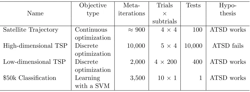
an efficient algorithm for optimizing a satellite's trajectory to monitor space debris. The second experiment involves the search for an algorithm that performs well on highly random traveling salesperson problems (TSP). The third experiment is also a TSP, but this time the cities occur on a ring and their distances are calculated from that. The last experiment tries to maximize the predictive accuracy on a classification problem. We summarize these experiments, their objectives, size, and purpose in Table 1.
In Table 1 ``objective type"" shows what the meta-optimization process was optimizing. The column titled ``meta-iterations"" describes how many unique algorithms were tried in
the search for the best algorithm for the task. ``Trials \times subtrials"" describes how many
ML and ATSD trials were conducted. Specifically, a trial refers to a specific configuration
meta-optimized algorithms found after the specified number of meta-iterations. Each resulting algorithm produced by the meta-optimization process was then tested across the number of tests listed in the ``tests"" column. Lastly, the column titled ``hypothesis,"" describes our hypothesized outcomes according to theory.
Throughout the course of conducting the experiments, we discovered multiple possible ways the meta-optimization process may fail, for both ML and ATSD. When the search for
optimizer algorithms or supervised learning algorithms is constrained (e.g., only adjusting
hyper-parameters), the algorithms may fail to exploit structure, which is embedded in the problem. This was demonstrated with the high-dimensional TSP; it has structure that the investigated optimizers have no capabilities to exploit. Another way for the process to fail is when the number of unique function evaluations is not fixed. Unless the number of unique function evaluations is fixed, some algorithms will use fewer unique function evaluations on
problems from \scrF - . The next problem is two fold: (1) the meta-optimization may fail to
return a near optimal algorithm for the approximate problem distribution ( \^\scrF + and \^\scrF - ),
and (2) this approximation of the problem distribution may be poor. Thus, the accuracy
of the approximation and the quality of the meta-optimization solution must be balanced;5
the optimal algorithm for a poor approximation is undesirable. These problems affect both ML and ATSD alike.
Below we describe each experiment in more detail, including the domain where the objective functions come from, the meta-optimization procedure, which common ML prac-tices we follow, individual tests within the experiment, and the computer setup. Results for each experiment are presented in Section 6. Just a quick note before delving into the first experiment. Whenever we say something is ``low-level,"" we are referring to the base optimization or learning problem. Similarly, if we mention something is ``meta-level"" we are referring to the meta-optimization required for ML and ATSD that optimizes the ``low-level"" algorithm.
5.1 Satellite Trajectory Problem
For the first experiment we use a physics based domain where the pilot problems involve monitoring space debris around a small artificial planet. Monitoring space debris presents a trade-off between the quality of observations and the time until revisiting the same debris. If the satellite were to have nearly the same orbit as a single piece of debris, then the satellite would pass by the debris slower and closer, resulting in higher quality observations. Similarly, a different orbit that is closer to or further from the planet would result in seeing the debris more frequently, but from further away. The low-level optimization objective is to find an orbit for a satellite that visits all debris within a specified distance and with minimal mean-time between visits.
We simplify the domain for the experiment in the following ways. Gravity of the planet is assumed to be uniform. Space debris are treated as points, meaning they have no physical size. Collisions are ignored. We use only 10 pieces of space debris to minimize simulation time. All orbits are in a two-dimensional space. Thus, an orbit's degrees of freedom are its: eccentricity (shape), orientation (angle of the ellipse), semi-major axis (size), and true
Table 2: Comparison of Pilot Problem Distributions
Data Set \scrF + \scrF -
Semi-Major Axis \sim N(400km,30km) half from \sim N(520km,30km)
half from \sim N(280km,30km)
Eccentricity \sim N(0.1,0.1) \sim Exp(1/3), but \leq 1.0
True Anomaly \sim U(0,2\pi ) \sim U(\pi /4,7\pi /4)
Orientation \sim U(0,2\pi ) \sim U(\pi /2,2\pi )
anomaly (phase of the orbit). In spite of these simplifications and the fact all the variables are continuous, the multiple pieces of space debris introduce many local extrema.
Recall that our methods discussed in Section 3.1 require multiple objective functions. We create multiple instantiations of problems from this domain. Each problem has space debris in a different configuration, but drawn from one of two distributions. These distributions
correspond to \scrF + and\scrF - . More details can be found in Table 2. To ensure there were no
large gaps, we used Latin hypercube sampling (McKay et al., 1979).
5.1.1 Meta-Optimization Procedure
The meta-level problem that we investigate is the meta-optimization of an optimizer. We chose to use Matlab's simulated annealing (SA) procedure as our low-level optimizer. SA was chosen for this experiment due to its large number of hyper-parameters and behavior dependent upon these hyper-parameters (Ingber, 1993, 1996). The hyper-parameters we investigate are:
\bullet step length function (two choices),
\bullet initial temperatures (four real numbers),
\bullet cooling function (three choices),
\bullet reannealing time (one integer),
\bullet upper bounds (four real numbers), and
\bullet lower bounds (four real numbers).
The meta-optimization procedure is designed to find an optimizer that quickly minimizes the mean-time between the satellite visiting debris and the satellite's closest approach to each piece of debris. It does this by searching for good values for the above
hyper-parameters. We searched for hyper-parameters that produce a low cumulative
objec-tive value, meaning finding a lower objecobjec-tive value sooner was preferred (i.e., \Phi \bigl( dym
\bigr) =
\sum m
i=1min\{ d y i\} ).
The meta-optimization consisted of three phases: differentiation, SA optimization, and a local search. The starting hyper-parameters were differentiated using SA for 35 iterations. While we recorded only the best solution during these 35 iterations, all remaining optimization iterations were recorded. Then, SA was used to further investigate the
hyper-parameters, due to its global search properties.6 Last, a gradient descent method (Matlab's
Table 3: Four Types of Trials
Methods ATSD+ML3 ML9 ML3 Control
\bigm| \bigm| \bigm|
\^
\scrF +
\bigm| \bigm|
\bigm| 3 9 3 1
\bigm| \bigm| \bigm|
\^
\scrF - \bigm| \bigm|
\bigm| 9 0 0 0
Subtrials 4 4 1 1
Control? No No Yes Yes
\ttf \ttm \tti \ttn \ttc \tto \ttn ) was used to finish the search process. We discovered that gradient descent worked
well to search for real-valued hyper-parameters on this particular problem. The
meta-optimization problem was setup to minimize the median of \^\scrF + and maximize the median
of \^\scrF - . We used \beta =1/3, because our ATSD+ML test uses three times as many sacrificial
functions as probable functions.
5.1.2 Practices Followed
One common practice involves searching for hyper-parameters (e.g., model selection) to minimize the bootstrap- or cross-validation error (Kohavi, 1995; Arlot and Celisse, 2010). Following these practices, we tested ATSD+ML according to (8), to search for good hyper-parameters for an optimization procedure on a collection of pilot problems. However, our experiment differs in three key aspects from common practice. First, we only test (i.e., judge the final performance) against data the optimizer has never seen, as stipulated by Wolpert (2001); Giraud-Carrier and Provost (2005). Second, the meta-optimization occurs across multiple objective functions from a limited domain, as advised by Giraud-Carrier and Provost (2005). Another common practice we purposefully chose to ignore is the partitioning of the data into training, probe/validation, and test partitions. We only use training and test partitions. The reason for this is the need to test if ATSD+ML limits the effects of overtraining. We test the algorithms from only the final iteration for the same reason.
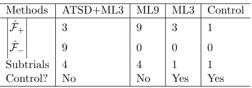
5.1.3 Trials
We conduct four types of trials, summarized in Table 3: ATSD+ML3, ML with three samples (ML3), ML with nine samples (ML9), and a control where no ML nor ATSD are
applied. ML9's \^\scrF + consisted of nine sample problems. ML3 and ATSD+ML3 share a
subset of ML9's \^\scrF +. The control uses one problem from the set ATSD+ML3 and ML3
share. We chose these trials to demonstrate how performance can be improved. The ML3
performance could be improved by either increasing the number of samples from\scrF + (ML9)
or by introducing ATSD (ATSD+ML3). Both these alternatives are tested four times. Each algorithm generated from the table is then tested against 100 samples of never seen before
data from the\scrF + distribution. We leave the analysis over\scrF 0 for another experiment.
5.1.4 Experiment Computer Setup
processor and the third using the Intel i7-3770K quad-core processor. All computers have 4GB of RAM (DDR2 800, DDR3 1033, DDR3 1600). All file I/O is carried out using a virtual drive hosted over the Internet. Both results and computations that could be reused are saved to the virtual drive. Two of the three computers run Matlab on Windows 7. The third computer runs Matlab in Ubuntu.
We acknowledge that this hardware is now dated and that there are better suited environments that should, and will, be used in the future. However, due to the lengthy process to gain access to high performance computing clusters, we only use a small cluster here. Anyone wishing to reproduce the results or to extend them will easily be able to use the coarse-grain parallelism that we built into our code to exploit larger clusters.
The meta-optimization code is written to exploit coarse-grain parallelism, to take advantage of each core available, while avoiding the need to use Matlab's parallel computing toolbox. Each computer performs meta-optimization for one of the ATSD+ML3, ML9, and ML3 trials. To keep one computer responsive for daily tasks, only one trial was performed on ML3. The control case did not use any meta-optimization.
The meta-optimization process takes about 1.5 months to finish for the ML3 experiment, about 4.5 months to finish the ML9 experiment, and approximately 6.0 months to complete
the ATSD+ML3 experiment. After six months, we collect about 1.7 GB of data.7 After the
meta-optimization, we run the algorithms over 100 different problems from the\scrF +to collect
statistical performance data. Each algorithm takes about 10 hours to run over this set of 100 problems. Due to how relatively quick it is to test an algorithm over 100 problems, we did not need to partition the trials over the cluster. This generates another 1.4 GB of data over the course of a week. All 3.1 GB of the data is available, but we also offer just the Matlab scripts (only 100KB) that can generate statistically similar data.
Because the meta-optimization run times were deemed too slow to reproduce statistically similar results, we found ways to improve the execution speed. Since the core kernel of the simulation is already optimized and Matlab's ODE45 was still the bottleneck (taking over 98\% of the time), we copied the ODE45 code and removed all the code for options. Further improvements were made by turning off Matlab's ODE45's interpolation, as we were already interpolating ODE45 results at specific points.
These changes give us approximately a 2x speedup in total. Trimming the ODE45 code improves the speed by about 50\%. We are surprised how much this helps; we attribute it to avoiding the majority of the ODE45's if-branches, removing its switch statement, and reduction in code size. Turning off Matlab's ODE45's interpolation provides another 30\% speed up. With modern hardware and these revisions, it should take only approximately two months to produce statistically similar results.
5.2 High Dimensional Traveling Salesperson Problems
In this experiment we try to demonstrate that theory correctly predicts when ATSD should fail. Theory predicts that if ML fails, then so should ATSD. We believe this is an important experiment as it tries to disprove the theory from the opposite direction; we would be
Table 4: Correlation Matrix by Problem Distribution
\scrF + \scrF 0 \scrF - \Sigma i,j = (1+2.82| i - j| )2 | i - 0.5j| 2 \delta (i, j)
surprised to find that ATSD works where ML fails. ML and ATSD require structure in the input-output pairs. Structure, only in the problem itself but not the input-output pairs, is of little use for an optimizer or learner unless one is attempting to discover the underlying
problem (e.g., the TSP cost matrix) and then solve it with a non-black-box solver. This is
actually one method discussed in (Culberson, 1998).
For all TSP problems in this experiment, we limit the input to only valid sequences of cities. Thus, the entire input space is valid. Only total distance traveled is analyzed. No information from partial solutions is used. The problem distributions are generated with the following technique:
\bullet For each row of the cost matrix, sample a 20 dimensional multivariate normal
distri-bution.
\bullet Compose a cost matrix from 20 such samples.
\bullet Make the cost matrix symmetric by adding it to its own transpose.
\bullet The minimum value is set to zero.
The covariance matrix is defined in Table 4. \scrF + has a nearly singular covariance matrix,
producing 20 random numbers, which approximately follow a random walk.8 Before making
the cost matrix symmetric, each row is an independent sample. This structure is not
readily exploitable by the low-level optimizer. The low-level optimizer avoids analyzing
trends in these random walks. \scrF - produces a random cost matrix where each element is
independently normally distributed. We will assume this is sufficient to make the probability
of particular outputs independent of the inputs, implyingP(f) =\prod
xP(y=f(x)).
5.2.1 Meta-Optimization Procedure
The meta-optimization problem is to find the hyper-parameters for a custom genetic algorithm. The hyper parameters include five initial paths, a mutation rate, a max swap-size schedule, and a swap-swap-size parameter. The initial paths and mutation rate should be self-explanatory. The swap-size parameter defines a random variable distributed according to the exponential distribution, but this value is clamped to never exceed the max swap-size. The max swap-size schedule provides 10 maximum values, each one valid for 10\% of the low-level optimization procedure. The clamped exponentially distributed swap-size determines how many cities are swapped at once.
The custom genetic algorithm primarily differs from a traditional genetic algorithm
in that it only generates valid inputs for the TSP problems. Random mutations are
implemented as random swaps. The crossover operation uses the differences in the paths
Table 5: Five Types of Trials
Methods ML5 ML10 ML15 ATSD250+ML5 ATSD250+ML5 Weak
\bigm| \bigm| \bigm|
\^
\scrF +
\bigm| \bigm|
\bigm| 5 10 15 5 5
\bigm| \bigm| \bigm|
\^
\scrF - \bigm| \bigm|
\bigm| 0 0 0 250 250
Subtrials 4 4 4 4 4
\beta 0 0 0 1 0.2
of the two top performing individuals to guide which cities to swap. We use a population size of five. At the time the experiment was run, the implementation permitted duplicate individuals. This means it is probable that the number of unique function evaluations differ for all trials; this is significant since any subtrial may be put at a disadvantage by exploring fewer possible solutions. However, considering the cost to rerun the experiment, we still present the results. A future experiment should retest this experiment with the number of unique function evaluations fixed. The number of unique function evaluations is made more consistent for the ring-based TSP experiment.
We chose to use Matlab's SA algorithm to perform the meta-optimization, primarily due to its global search property. Any global search meta-optimization routine could be used instead. Instead of using (8) verbatim, we replace the sums with averages. This allows us to vary
\bigm| \bigm| \bigm|
\^
\scrF +
\bigm| \bigm|
\bigm| and
\bigm| \bigm| \bigm|
\^
\scrF - \bigm| \bigm|
\bigm| while continuing to give the same relative importance\beta .
5.2.2 Practices Followed
We followed the same practices as discussed in Section 5.1.2.
5.2.3 Trials
We conduct five types of trials, outlined in Table 5: ML5, ML10, ML15, ATSD250+ML5,
and ATSD250+ML5 Weak. ML5 can be viewed as the control. We chose the trials
ML5, ML10, and ML15 to demonstrate the effects of increasing \bigm| \bigm| \bigm| \scrF \^+
\bigm| \bigm|
\bigm| on a domain where
little to no patterns should be exploitable. The ATSD+ML trials, ATSD250+ML5 and ATSD250+ML5 Weak, demonstrate the effects of using random TSP problems for sacrificial data at differing weights of ML compared to ATSD.
Four subtrials are conducted per trial, all using the same \^\scrF +, \^\scrF - , or both. The subtrials
only differ in the random seed used in the meta-optimization process (i.e., the simulated
annealing random seed). This is designed to roughly estimate the variability of the quality of the algorithms returned from the meta-optimization process. Since we hypothesize ATSD and ML should fail, we want to give every chance for ML and ATSD to work. So we use 10,000 simulated annealing iterations to have a greater chance to exploit structure that only
works on \^\scrF +.
We test each resulting algorithm (a total of 20 algorithms) against 10,000 samples of
−1 −0.5 0 0.5 1 −1
−0.8 −0.6 −0.4 −0.2 0 0.2 0.4 0.6 0.8 1
F0city distribution
x location
y
lo
c
a
ti
o
n
(a) The\scrF 0city distribution
−1 −0.5 0 0.5 1
−1 −0.8 −0.6 −0.4 −0.2 0 0.2 0.4 0.6 0.8 1
F+city distribution
x location
y
lo
c
a
ti
o
n
(b) The\scrF + city distribution
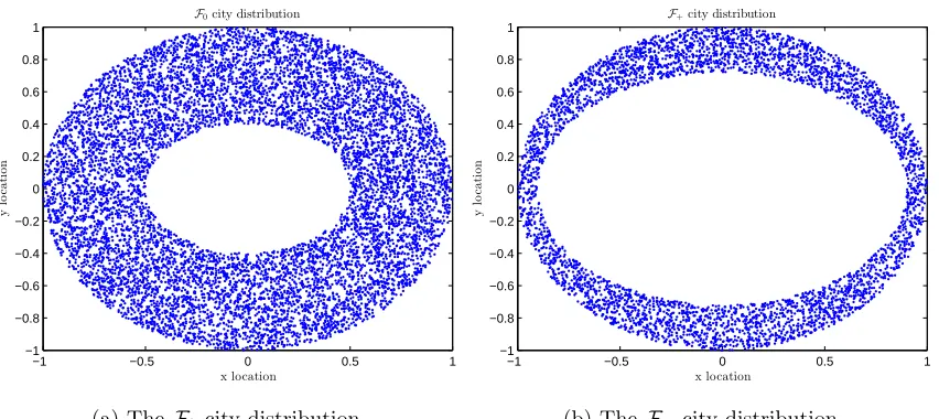
Figure 1: City distributions by problem distribution
5.2.4 Computer setup
The computer setup is very similar to that described in Section 5.1.4. We only use the first two computers as this experiment ran faster, taking only about three days to complete. We use the same Internet based virtual drive for all I/O. The meta-optimization process generates about 963 MB of data including checkpointing every 50 iterations. The code is written to exploit coarse-grain parallelism, scaling up to about 20 instances of Matlab (avoids using the Matlab parallel computing toolbox).
5.3 Traveling Salesperson on a Ring
In this experiment, we investigate ATSD and ML over a discrete optimization problem where multiple properties from the domain should be exploitable. This experiment is in contrast to the high dimensional TSP. As in the previous experiment, we limit the input to only valid sequences of cities. Thus, all input is valid. Only the total distance traveled is analyzed. No information from partial solutions is used. However, rather than generate a correlated cost matrix from random values directly, the cities are randomly placed on a ring
and their cost values are computed as the Euclidean distance between cities (cf. Figure 1).
As the ring's inner and outer diameter become the same, the optimal path converges to traveling in a circular loop. Furthermore, cities are labeled in a clockwise fashion.
The problem distribution comes from the following. \scrF + comes from a narrow ring (cf.
Figure 1b). \scrF 0comes from a wide ring (cf. Figure 1a). \scrF - are TSP problems with randomly
generated cost matrices, similar to the\scrF - in the previous experiment (the high dimensional
TSP experiment).
5.3.1 Meta-Optimization Procedure
Table 6: Four Types of Trials
Methods ML5 ML10 ATSD15+ML5 ATSD50+ML5
\bigm| \bigm| \bigm|
\^
\scrF +
\bigm| \bigm|
\bigm| 5 10 5 5
\bigm| \bigm| \bigm|
\^
\scrF - \bigm| \bigm|
\bigm| 0 0 15 50
Subtrials 200 200 200 200
\beta 0 0 0.2 0.2
swap-size schedule, and swap-size parameter. We use the same custom genetic algorithm as before, with two exceptions. First, we modify the low-level algorithm to force all individuals in the population to represent unique paths. Duplicate paths are replaced with random paths. Because this slows down the low-level algorithm to about half its original speed, we further optimize the low-level algorithm to nearly restore its original performance. We still use Matlab's SA algorithm to find the hyper-parameters. The sums are still replaced with the averages in (8).
5.3.2 Practices Followed
We follow the same practices as discussed in Section 5.1.2.
5.3.3 Trials
We conduct four types of trials, summarized in Table 6: ML5, ML10, ATSD15+ML5, and ATSD50+ML5. ML5 can be viewed as the control. We chose the trials ML5 and ML10 to demonstrate the effects of increasing
\bigm| \bigm| \bigm|
\^
\scrF +\bigm| \bigm|
\bigm| . The ATSD+ML trials, ATSD15+ML5 and
ATSD50+ML5, demonstrate the effects of increasing the number of random TSP problems.
200 subtrials are conducted per trial, all using the same \^\scrF +, \^\scrF - , or both. The subtrials
only differ in the random seed used in the meta-optimization process (i.e., the simulated
annealing random seed). This is designed to accurately estimate the variability of the
quality of the algorithms returned from the meta-optimization process. Because we are using a total of 800 subtrials, we limit the meta-optimization search to 2,000 simulated annealing iterations for time considerations.
We test each resulting algorithm (a total of 800 algorithms) against 400 samples of never
seen before data from the \scrF +,\scrF 0, and \scrF - distributions.
5.3.4 Computer setup
The computer setup is very similar to that described in Section 5.1.4. We only use the first two computers as this experiment took only about one week to complete. We use the same Internet based virtual drive for all I/O. The meta-optimization process generates about 1020 MB of data including checkpointing every 100 iterations. The code is written to exploit
coarse-grain parallelism, scaling up to about 800 instances of Matlab. Our parallelism
5.4 Classification Problem
This experiment tests ATSD+ML against a supervised machine learning problem. Specif-ically, the task is to learn to classify whether an individual makes more than \$50K per year based on 14 attributes such as the sector in which the person works (private, local government, state government, etc.), job type, level of education, sex, age, hours per week, native-country, etc. This data, referred to as the ``adult"" data, is made publicly available and can be found in the UCI Machine Learning Repository (Bache and Lichman, 2013).
This experiment's goal is to demonstrate how ATSD can be used to boost machine learning performance, not to beat previous classification performance. We compare the classification accuracy of support vector machines (SVMs). The kernel and its parameters are meta-optimized using differing numbers of cross-validation samples and sacrificial
prob-lems. Cross-validations are used for \^\scrF +, which is arguably insufficient (Wolpert, 2001).
This is not so much a drawback for the experiment as it demonstrates how quality \^\scrF + may
be difficult to obtain, further motivating the use of ATSD.
We use three types of sacrificial data. One third of \^\scrF - uses real tuples of the attributes,
but with random classification results. Another third of \^\scrF - uses both random tuples of
attributes and classification results. The last third of \^\scrF - uses real tuples of attributes,
but with a very simple classification problem where the result is wholly determined by a logical conjunction based on the sex, age, and number of years of education. This third set of sacrificial data exhibits several properties absent in the actual data: it is noise free, it depends only on three parameters (ignoring important information such as the job type) and has very low Kolmogorov complexity.
5.4.1 Meta-Optimization Procedure
The meta-optimization objective is to find a good set of SVM hyper-parameters. Specifically, the SVM's kernel, box constraint (training error versus complexity), and kernel parameters
(e.g. Gaussian kernel width). We investigate seven SVM kernels including:
\bullet Linear: u\intercal v
\bullet Gaussian: exp( - | u - v| 2/(2\sigma 2))
\bullet Laplace: exp( - | u - v| /\sigma )
\bullet Cauchy: (1 +| u - v| 2/\sigma 2) - 1
\bullet Tanh (Multilayer Perception): tanh(\alpha u\intercal v+c)
\bullet Inhomogeneous polynomial: (\alpha u\intercal v+c)p
\bullet Logarithmic kernel: - log(c+| x - y| p).9
\sigma ,\alpha ,c, and p in this context are kernel parameters. u and v are data. Note that some of
these kernels are only conditionally positive definite. Meaning, if used, the SVM may fail to converge to globally optimal results.