High-dimensional Covariance Estimation Based On Gaussian Graphical Models

High-dimensional Covariance Estimation Based On

Gaussian Graphical Models

Shuheng Zhou SHUHENGZ@UMICH.EDU

Department of Statistics University of Michigan

Ann Arbor, MI 48109-1041, USA

Philipp R ¨utimann RUTIMANN@STAT.MATH.ETHZ.CH

Seminar for Statistics ETH Z¨urich

8092 Z¨urich, Switzerland

Min Xu MINX@CS.CMU.EDU

Machine Learning Department Carnegie Mellon University Pittsburgh, PA 15213-3815, USA

Peter B ¨uhlmann BUHLMANN@STAT.MATH.ETHZ.CH

Seminar for Statistics

ETH Z¨urich

8092 Z¨urich, Switzerland

Editor: Hui Zou

Abstract

Undirected graphs are often used to describe high dimensional distributions. Under sparsity condi-tions, the graph can be estimated usingℓ1-penalization methods. We propose and study the follow-ing method. We combine a multiple regression approach with ideas of thresholdfollow-ing and refittfollow-ing: first we infer a sparse undirected graphical model structure via thresholding of each among many ℓ1-norm penalized regression functions; we then estimate the covariance matrix and its inverse using the maximum likelihood estimator. We show that under suitable conditions, this approach yields consistent estimation in terms of graphical structure and fast convergence rates with respect to the operator and Frobenius norm for the covariance matrix and its inverse. We also derive an explicit bound for the Kullback Leibler divergence.

1. Introduction

There have been a lot of recent activities for estimation of high-dimensional covariance and inverse covariance matrices where the dimension p of the matrix may greatly exceed the sample size n. High-dimensional covariance estimation can be classified into two main categories, one which relies on a natural ordering among the variables [Wu and Pourahmadi, 2003; Bickel and Levina, 2004; Huang et al., 2006; Furrer and Bengtsson, 2007; Bickel and Levina, 2008; Levina et al., 2008] and one where no natural ordering is given and estimators are permutation invariant with respect to indexing the variables [Yuan and Lin, 2007; Friedman et al., 2007; d’Aspremont et al., 2008; Banerjee et al., 2008; Rothman et al., 2008]. We focus here on the latter class with permutation invariant estimation and we aim for an estimator which is accurate for both the covariance matrixΣ and its inverse, the precision matrixΣ−1. A popular approach for obtaining a permutation invariant estimator which is sparse in the estimated precision matrixbΣ−1is given by theℓ1-norm regularized maximum-likelihood estimation, also known as the GLasso [Yuan and Lin, 2007; Friedman et al., 2007; Banerjee et al., 2008]. The GLasso approach is simple to use, at least when relying on publicly available software such as the glasso package in R. Further improvements have been reported when using some SCAD-type penalized maximum-likelihood estimator [Lam and Fan, 2009] or an adaptive GLasso procedure [Fan et al., 2009], which can be thought of as a two-stage procedure. It is well-known from linear regression that such two- or multi-stage methods effectively address some bias problems which arise fromℓ1-penalization [Zou, 2006; Cand`es and Tao, 2007; Meinshausen, 2007; Zou and Li, 2008; B¨uhlmann and Meier, 2008; Zhou, 2009, 2010a].

There are a few key motivations and consequences for proposing such an approach based on graph-ical modeling. We will theoretgraph-ically show that there are cases where our graph based method can accurately estimate conditional independencies among variables, that is, the zeroes ofΣ−1, in sit-uations where GLasso fails. The fact that GLasso easily fails to estimate the zeroes of Σ−1 has been recognized by Meinshausen [2008] and it has been discussed in more details in Ravikumar et al. [2011]. Closer relations to existing work are primarily regarding our first stage of estimating the structure of the graph. We follow the nodewise regression approach from Meinshausen and B¨uhlmann [2006] but we make use of recent results for variable selection in linear models assuming the much weaker restricted eigenvalue condition [Bickel et al., 2009; Zhou, 2010a] instead of the restrictive neighborhood stability condition [Meinshausen and B¨uhlmann, 2006] or the equivalent irrepresentable condition [Zhao and Yu, 2006]. In some sense, the novelty of our theory extending beyond Zhou [2010a] is the analysis for covariance and inverse covariance estimation and for risk consistency based on an estimated sparse graph as we mentioned above. Our regression and thresh-olding results build upon analysis of the thresholded Lasso estimator as studied in Zhou [2010a]. Throughout our analysis, the sample complexity is one of the key focus point, which builds upon results in Zhou [2010b]; Rudelson and Zhou [2011]. Once the zeros are found, a constrained max-imum likelihood estimator of the covariance can be computed, which was shown in Chaudhuri et al. [2007]; it was unclear what the properties of such a procedure would be. Our theory answers such questions. As a two-stage method, our approach is also related to the adaptive Lasso [Zou, 2006] which has been analyzed for high-dimensional scenarios in Huang et al. [2008], Zhou et al. [2009] and van de Geer et al. [2011]. Another relation can be made to the method by R¨utimann and B¨uhlmann [2009] for covariance and inverse covariance estimation based on a directed acyclic graph. This relation has only methodological character: the techniques and algorithms used in R¨utimann and B¨uhlmann [2009] are very different and from a practical point of view, their ap-proach has much higher degree of complexity in terms of computation and implementation, since estimation of an equivalence class of directed acyclic graphs is difficult and cumbersome. There has also been work that focuses on estimation of sparse directed Gaussian graphical model. Verze-len [2010] proposes a multiple regularized regression procedure for estimating a precision matrix with sparse Cholesky factors, which correspond to a sparse directed graph. He also computes non-asymptotic Kullback Leibler risk bound of his procedure for a class of regularization functions. It is important to note that directed graph estimation requires a fixed good ordering of the variables a priori.

1.1 Notation

determinant of W , tr(W) the trace of W . Let ϕmax(W) andϕmin(W) be the largest and smallest eigenvalues, respectively. We write diag(W)for a diagonal matrix with the same diagonal as W and

offd(W) =W₋diag(W). The matrix Frobenius norm is given by_kW_kF=q∑i∑jw2i j. The operator

norm_kW_k2₂ is given byϕmax(WWT). We write_{| · |}1for theℓ1norm of a matrix vectorized, that is, for a matrix_|W_|1=kvecWk1=∑i∑j|wi j|, and sometimes writekWk0for the number of non-zero entries in the matrix. For an index set T and a matrix W = [wi j], write WT ≡(wi jI((i,j)∈T)),

where I(_·)is the indicator function.

2. The Model and the Method

We assume a multivariate Gaussian model

X= (X1, . . . ,Xp)∼

N

p(0,Σ0), where Σ0,ii=1. (1)

The data is generated by X(1), . . . ,X(n)i.i.d._∼

N

_p(0,Σ0). Requiring the mean vector and all vari-ances being equal to zero and one respectively is not a real restriction and in practice, we can easily center and scale the data. We denote the concentration matrix byΘ0=Σ−₀1.

Since we will use a nodewise regression procedure, as described below in Section 2.1, we consider a regression formulation of the model. Consider many regressions, where we regress one variable against all others:

Xi=

∑

j6=i

βi

jXj+Vi(i=1, . . . ,p), where (2)

Vi∼

N

(0,σV2i)independent of{Xj; j6=i}(i=1, . . . ,p). (3)

There are explicit relations between the regression coefficients, error variances and the concentration matrixΘ0= (θ0,i j):

βi

j=−θ0,i j/θ0,ii,Var(Vi):=σV2i =1/θ0,ii(i,j=1, . . . ,p). (4)

Furthermore, it is well known that for Gaussian distributions, conditional independence is encoded inΘ0, and due to (4), also in the regression coefficients:

Xiis conditionally dependent of Xjgiven{Xk; k∈ {1, . . . ,p} \ {i,j}}

⇐⇒ θ0,i j6=0 ⇐⇒ βij6=0 andβij6=0. (5)

For the second equivalence, we assume that Var(Vi) =1/θ0,ii>0 and Var(Vj) =1/θ0,j j>0.

Con-ditional (in-)dependencies can be conveniently encoded by an undirected graph, the conCon-ditional independence graph which we denote by G= (V,E0). The set of vertices is V ={1, . . . ,p}and the set of undirected edges E0⊆V×V is defined as follows:

there is an undirected edge between nodes i and j

⇐⇒ θ0,i j6=0 ⇐⇒ βij6=0 andβ i

Note that on the right hand side of the second equivalence, we could replace the word ”and” by ”or”. For the second equivalence, we assume Var(Vi),Var(Vj)>0 following the remark after (5).

We now define the sparsity of the concentration matrixΘ0 or the conditional independence graph. The definition is different than simply counting the non-zero elements of Θ0, for which we have supp(Θ0) = p+2_|E0|. We consider instead the number of elements which are sufficiently large. For each i, define the number si_0,nas the smallest integer such that the following holds:

p

∑

j=1,j₆=i

min_{θ2_{0,i j},λ2θ0,ii} ≤ si0,nλ2θ0,ii, where λ=

p

2 log(p)/n, (7)

where essential sparsity si_0,n at row i describes the number of “sufficiently large” non-diagonal elementsθ0,i j relative to a given(n,p)pair andθ0,ii,i=1, . . . ,p. The value S0,nin (8) is summing essential sparsity across all rows ofΘ0,

S0,n := p

∑

i=1

si_0,n. (8)

Due to the expression of λ, the value of S0,n depends on p and n. For example, if all non-zero

non-diagonal elementsθ0,i j of the ith row are larger in absolute value thanλpθ0,ii, the value si_0,n

coincides with the node degree si. However, if some (many) of the elements_|θ0,i j|are non-zero

but small, si_0,n is (much) smaller than its node degree si; As a consequence, if some (many) of

|θ0,i j|,∀i,j,i6= j are non-zero but small, the value of S0,nis also (much) smaller than 2|E0|, which is the “classical” sparsity for the matrix(Θ0₋diag(Θ0)). See Section A for more discussions.

2.1 The Estimation Procedure

The estimation of Θ0 andΣ0 =Θ−₀1 is pursued in two stages. We first estimate the undirected graph with edge set E0as in (6) and we then use the maximum likelihood estimator based on the estimateEbn, that is, the non-zero elements ofΘbncorrespond to the estimated edges inEbn. Inferring

the edge set E0can be based on the following approach as proposed and theoretically justified in Meinshausen and B¨uhlmann [2006]: perform p regressions using the Lasso to obtain p vectors of regression coefficientsbβ1, . . . ,bβp_{where for each i,}b_βi_={b_βi

j; j∈ {1, . . . ,p} \i}; Then estimate the

edge set by the “OR” rule,

estimate an edge between nodes i and j_⇐⇒bβi_j6=0 orbβ_ij₆=0. (9)

2.1.1 NODEWISEREGRESSIONS FORINFERRING THEGRAPH

In the present work, we use the Lasso in combination with thresholding [Zhou, 2009, 2010a]. Con-sider the Lasso for each of the nodewise regressions

βi

init=argminβi n

∑

r=1

(X_i(r)₋

∑

j6=i

βi jX

(r)

j )

2_+λ

n

∑

j6=i

whereλn>0 is the same regularization parameter for all regressions. Since the Lasso typically

es-timates too many components with non-zero estimated regression coefficients, we use thresholding to get rid of variables with small regression coefficients from solutions of (10):

b βi

j(λn,τ) =βij,init(λn)I(|βij,init(λn)|>τ), (11)

whereτ>0 is a thresholding parameter. We obtain the corresponding estimated edge set as defined by (9) using the estimator in (11) and we use the notation

b

En(λn,τ). (12)

We note that the estimator depends on two tuning parametersλnandτ.

The use of thresholding has clear benefits from a theoretical point of view: the number of false positive selections may be much larger without thresholding (when tuned for good prediction). and a similar statement would hold when comparing the adaptive Lasso with the standard Lasso. We refer the interested reader to Zhou [2009, 2010a] and van de Geer et al. [2011].

2.1.2 MAXIMUMLIKELIHOODESTIMATIONBASED ONGRAPHS

Given a conditional independence graph with edge set E, we estimate the concentration matrix by maximum likelihood. Denote bySbn=n−1∑nr=1X(r)(X(r))T the sample covariance matrix (using that the mean vector is zero) and by

b

Γn=diag(Sbn)−1/2(Sbn)diag(Sbn)−1/2

the sample correlation matrix. The estimator for the concentration matrix in view of (1) is:

b

Θn(E) =argmin_Θ∈Mp,E

tr(ΘbΓn)−log|Θ|

, where

M

_p,E =_{Θ_∈Rp×p_; Θ_{≻0 and}θ_{i j=0 for all(i,j)6∈E, where i6= j} (13)} defines the constrained set for positive definite Θ. If n_≥q∗ where q∗ is the maximal clique size of a minimal chordal cover of the graph with edge set E, the MLE exists and is unique, see, for example Uhler [2011, Corollary 2.3]. We note that our theory guarantees that n_≥q∗ holds with high probability for G= (V,E), where E=Ebn(λn,τ)), under Assumption (A1) to be introduced in

the next section. The definition in (13) is slightly different from the more usual estimator which uses the sample covarianceSbnrather thanΓbn. Here, the sample correlation matrix reflects the fact

that we typically work with standardized data where the variables have empirical variances equal to one. The estimator in (13) is constrained leading to zero-values corresponding to Ec=_{(i,j): i,j=1, . . . ,p,i₆= j,(i,j)_6∈E_}.

If the edge set E is sparse having relatively few edges only, the estimator in (13) is already suffi-ciently regularized by the constraints and hence, no additional penalization is used at this stage. Our final estimator for the concentration matrix is the combination of (12) and (13):

b

2.1.3 CHOOSING THEREGULARIZATION PARAMETERS

We propose to select the parameterλn via cross-validation to minimize the squared test set error

among all p regressions:

b_λn=argmin_λ

p

∑

i=1

(CV-score(λ) of ith regression),

where CV-score(λ) of ith regression is with respect to the squared error prediction loss. Sequentially proceeding, we then selectτby cross-validating the multivariate Gaussian log-likelihood, from (13). Regarding the type of cross-validation, we usually use the 10-fold scheme. Due to the sequential nature of choosing the regularization parameters, the number of candidate estimators is given by the number of candidate values for λplus the number of candidate value forτ. In Section 4, we describe the grids of candidate values in more details. We note that for our theoretical results, we do not analyze the implications of our method using estimatedbλnandbτ.

3. Theoretical Results

In this section, we present in Theorem 1 convergence rates for estimating the precision and the co-variance matrices with respect to the Frobenius norm; in addition, we show a risk consistency result for an oracle risk to be defined in (16). Moreover, in Proposition 4, we show that the model we select is sufficiently sparse while at the same time, the bias term we introduce via sparse approximation is sufficiently bounded. These results illustrate the classical bias and variance tradeoff. Our analysis is non-asymptotic in nature; however, we first formulate our results from an asymptotic point of view for simplicity. To do so, we consider a triangular array of data generating random variables

X(1), . . . ,X(n)i.i.d._∼

N

_p(0,Σ0),n=1,2, . . . (15)

whereΣ0=Σ0,nand p=pnchange with n. LetΘ0:=Σ−₀1. We make the following assumptions.

(A0) The size of the neighborhood for each node i_∈V is upper bounded by an integer s<p and the sample size satisfies for some constant C

n_≥Cs log(p/s).

(A1) The dimension and number of sufficiently strong non-zero edges S0,nas in (8) satisfy:

dimen-sion p grows with n following p=o(ecn)for some constant 0<c<1 and

S0,n=o(n/log max(n,p)) (n→∞).

(A2) The minimal and maximal eigenvalues of the true covariance matrix Σ0 are bounded: for some constants Mupp≥Mlow>0, we have

Moreover, throughout our analysis, we assume the following. There exists v2>0 such that for all i, and Vi as defined in (3): Var(Vi) =1/θ0,ii≥v2.

Before we proceed, we need some definitions. Define forΘ_≻0

R(Θ) =tr(ΘΣ0)₋log_|Θ_|, (16) where minimizing (16) without constraints givesΘ0. Given (8), (7), andΘ0, define

C_diag2 :=min_{ max

i=1,...pθ

2

0,ii,_imax

=1,...,p s i

0,n/S0,n

· kdiag(Θ0)_k2_F}. (17) We now state the main results of this paper. We defer the specification on various tuning parameters, namely,λn,τto Section 3.2, where we also provide an outline for Theorem 1.

Theorem 1 Consider data generating random variables as in (15) and assume that (A0), (A1), and (A2) hold. We assumeΣ0,ii=1 for all i. Then, with probability at least 1−d/p2, for some small constant d>2, we obtain under appropriately chosenλnandτ, an edge setEbnas in (12), such that |Eb_{n| ≤}2S0,n, where |Ebn\E0| ≤S0,n; (18) and forΘbnandΣbn= (Θbn)−1as defined in (14), the following holds,

bΘn−Θ0

2≤ k b

Θn−Θ0kF = OP

q

S0,nlog max(n,p)/n

,

bΣn−Σ0

2≤ kΣbn−Σ0kF = OP q

S0,nlog max(n,p)/n

,

R(Θbn)−R(Θ0) = OP(S0,nlog max(n,p)/n),

where the constants hidden in the OP() notation depend on τ, Mlow,Mupp, Cdiag as in (17), and

constants concerning sparse and restrictive eigenvalues ofΣ0(cf. Section 3.2 and B).

We note that convergence rates for the estimated covariance matrix and for predictive risk depend on the rate in Frobenius norm of the estimated inverse covariance matrix. The predictive risk can be interpreted as follows. Let X ∼

N

(0,Σ0)with fΣ0 denoting its density. Let fbΣ_n be the density

for

N

(0,Σbn) and DKL(Σ0kbΣn) denotes the Kullback Leibler (KL) divergence from

N

(0,Σ0) to

N

(0,bΣn). Now, we have forΣ,bΣn≻0, R(Θbn)−R(Θ0):=2E0

h

log fΣ0(X)−log fΣb_n(X)

i

:=2DKL(Σ0kΣbn)≥0. (19)

Actual conditions and non-asymptotic results that are involved in the Gelato estimation appear in Sections B, C, and D respectively.

Remark 2 Implicitly in (A1), we have specified a lower bound on the sample size to be n= Ω(S0,nlog max(n,p)). For the interesting case of p>n, a sample size of

is sufficient in order to achieve the rates in Theorem 1. As to be shown in our analysis, the lower bound on n is slightly different for each Frobenius norm bound to hold from a non-asymptotic point of view (cf. Theorem 19 and 20).

Theorem 1 can be interpreted as follows. First, the cardinality of the estimated edge set exceeds S0,n at most by a factor 2, where S0,n as in (8) is the number of sufficiently strong edges in the

model, while the number of false positives is bounded by S0,n. Note that the factors 2 and 1 can

be replaced by some other constants, while achieving the same bounds on the rates of convergence (cf. Section D.1). We emphasize that we achieve these two goals by sparse model selection, where only important edges are selected even though there are many more non-zero edges in E0, under conditions that are much weaker than (A2). More precisely, (A2) can be replaced by conditions on sparse and restrictive eigenvalues (RE) ofΣ0. Moreover, the bounded neighborhood constraint (A0) is required only for regression analysis (cf. Theorem 15) and for bounding the bias due to sparse approximation as in Proposition 4. This is shown in Sections B and C. Analysis follows from Zhou [2009, 2010a] with earlier references to Cand`es and Tao [2007], Meinshausen and Yu [2009] and Bickel et al. [2009] for estimating sparse regression coefficients.

We note that the conditions that we use are indeed similar to those in Rothman et al. [2008], with (A1) being much more relaxed when S0,n≪ |E0|. The convergence rate with respect to the Frobenius norm should be compared to the rate OP(

p

|E0|log max(n,p)/n)in case diag(Σ0)is known, which is the rate in Rothman et al. [2008] for the GLasso and for SCAD [Lam and Fan, 2009]. In the scenario where_|E0| ≫S0,n, that is, there are many weak edges, the rate in Theorem 1 is better than

the one established for GLasso [Rothman et al., 2008] or for the SCAD-type estimator [Lam and Fan, 2009]; hence we require a smaller sample size in order to yield an accurate estimate ofΘ0.

Remark 3 For the general case where Σ0,ii,i=1, . . . ,p are not assumed to be known, we could achieve essentially the same rate as stated in Theorem 1 for _kΘbn−Θ0k2 andkbΣn−Σ0k2 under (A0),(A1) and(A2) following analysis in the present work (cf. Theorem 6) and that in Rothman

et al. [2008, Theorem 2]. Presenting full details for such results are beyond the scope of the current paper. We do provide the key technical lemma which is essential for showing such bounds based on estimating the inverse of the correlation matrix in Theorem 6; see also Remark 7 which immediately follows.

In this case, for the Frobenius norm and the risk to converge to zero, a too large value of p is not allowed. Indeed, for the Frobenius norm and the risk to converge,(A1)is to be replaced by:

(A3) p_≍nc for some constant 0<c<1 and p+S0,n=o(n/log max(n,p)) as n→∞. In this case, we have

kΘbn−Θ0kF = OP

q

(p+S0,n)log max(n,p)/n

,

kbΣn−Σ0kF = OP

q

(p+S0,n)log max(n,p)/n

,

Moreover, in the refitting stage, we could achieve these rates with the maximum likelihood estimator based on the sample covariance matrixSbnas defined in (20):

b

Θn(E) =argmin_Θ∈Mp,E

tr(ΘSbn)−log|Θ|

, where

M

_p,E =_{Θ_∈Rp×p_; Θ_{≻0 and}θ_{i j=0 for all(i,j)6∈E, where i6= j}. (20)}

A real high-dimensional scenario where p_≫n is excluded in order to achieve Frobenius norm consistency. This restriction comes from the nature of the Frobenius norm and when considering, for example, the operator norm, such restrictions can indeed be relaxed as stated above.

It is also of interest to understand the bias of the estimator caused by using the estimated edge set

b

Eninstead of the true edge set E0. This is the content of Proposition 4. For a givenEbn, denote by

e

Θ0=diag(Θ0) + (Θ0)_Eb

n =diag(Θ0) +Θ0,Ebn∩E0,

where the second equality holds sinceΘ0,Ec

0 =0. Note that the quantityΘ0e is identical toΘ0onEbn

and on the diagonal, and it equals zero onEb_nc=_{(i,j): i,j=1, . . . ,p,i₆= j,(i,j)_6∈Ebn}. Hence, the

quantityΘ0_,D :=Θ0e −Θ0measures the bias caused by a potentially wrong edge set Ebn; note that

e

Θ0=Θ0ifEbn=E0.

Proposition 4 Consider data generating random variables as in expression (15). Assume that (A0), (A1), and (A2) hold. Then we have for choices onλn,τas in Theorem 1 andEbnin (12),

Θ0,D_F :=kΘ0e −Θ0kF =OP

q

S0,nlog max(n,p)/n

.

We note that we achieve essentially the same rate for _k(Θ0e )−1₋Σ0_k

F; see Remark 27. We give

an account on how results in Proposition 4 are obtained in Section 3.2, with its non-asymptotic statement appearing in Corollary 17.

3.1 Discussions and Connections to Previous Work

It is worth mentioning that consistency in terms of operator and Frobenius norms does not depend too strongly on the property to recover the true underlying edge set E0in the refitting stage. Regard-ing the latter, suppose we obtain with high probability the screenRegard-ing property

E0⊆E, (21)

Theorem 5 Consider data generating random variables as in expression (15) and assume that (A1) and (A2) hold, where we replace S0,nwith S :=|E0|=∑_ip₌₁si. We assumeΣ0,ii=1 for all i. Suppose on some event

E

, such thatP₍

E

)_≥1₋d/p2for a small constant d, we obtain an edge set E such that E0⊆E and|E\E0|=O(S). Let Θbn(E)be the minimizer as defined in (13). Then, we have kΘbn(E)−Θ0kF =OP

p

S log max(n,p)/n.

It is clear that this bound corresponds to exactly that of Rothman et al. [2008] for the GLasso estimation under appropriate choice of the penalty parameter for a generalΣ_≻0 withΣii=1 for all i (cf. Remark 3). We omit the proof as it is more or less a modified version of Theorem 19, which proves the stronger bounds as stated in Theorem 1. We note that the maximum node-degree bound in (A0) is not needed for Theorem 5.

We now make some connections to previous work. First, we note that to obtain with high probability the exact edge recovery, E=E0, we need again sufficiently large non-zero edge weights and some restricted eigenvalue (RE) conditions on the covariance matrix as defined in Section A even for the multi-stage procedure. An earlier example is shown in Zhou et al. [2009], where the second stage estimatorbβcorresponding to (11) is obtained with nodewise regressions using adaptive Lasso [Zou, 2006] rather than thresholding as in the present work in order to recover the edge set E0with high probability under an assumption which is stronger than (A0). Clearly, given an accurateEbn, under

(A1) and (A2) one can then apply Theorem 5 to accurately estimate Θbn. On the other hand, it is

known that GLasso necessarily needs more restrictive conditions onΣ0than the nodewise regression approach with the Lasso, as discussed in Meinshausen [2008] and Ravikumar et al. [2011] in order to achieve exact edge recovery.

Furthermore, we believe it is straightforward to show that Gelato works under the RE conditions on Σ0and with a smaller sample size than the analogue without the thresholding operation in order to achieve nearly exact recovery of the support in the sense that E0⊆Ebnand maxi|Ebn,i\E0,i|is small,

that is, the number of extra estimated edges at each node i is bounded by a small constant. This is shown essentially in Zhou [2009, Theorem1.1] for a single regression. Given such properties of

b

En, we can again apply Theorem 5 to obtainΘbn under (A1) and (A2). Therefore, Gelato requires

relatively weak assumptions onΣ0in order to achieve the best sparsity and bias tradeoff as illustrated in Theorem 1 and Proposition 4 when many signals are weak, and Theorem 5 when all signals in E0 are strong.

Finally, it would be interesting to derive a tighter bound on the operator norm for the Gelato estima-tor. Examples of such bounds have been recently derived for a restricted class of inverse covariance matrices in Yuan [2010] and Cai et al. [2011].

3.2 An Outline for Theorem 1

the lower bounds for d0, D4, and hence also that forλn and t0that appear below. We simplify our notation in this section to keep it consistent with our theoretical non-asymptotic analysis to appear toward the end of this paper.

3.2.1 REGRESSION

We choose for some c0≥4

√

2, 0<θ<1, andλ=p2 log(p)/n,

λn=d0λ, where d0≥c0(1+θ)2 p

ρmax(s)ρmax(3s0).

Letβi_init,i=1, . . . ,p be the optimal solutions to (10) with λn as chosen above. We first prove an

oracle result on nodewise regressions in Theorem 15.

3.2.2 THRESHOLDING

We choose for some constants D1,D4to be defined in Theorem 15,

t0= f0λ:=D4d0λ where D4≥D1

and D1 depends on restrictive eigenvalue of Σ0; Apply (11) with τ=t0 and βiinit,i=1, . . . ,p for thresholding our initial regression coefficients. Let

D

i=_{j : j₆=i,βi_j,init<t0=f0λ},

where bounds on

D

i_{,i=1, . . . ,p are given in Lemma 16. In view of (9), we let}

D

=_{(i,j): i=₆ j :(i,j)_∈

D

i ∩

D

j

}. (22)

3.2.3 SELECTINGEDGESETE

Recall for a pair(i,j)we take the OR rule as in (9) to decide if it is to be included in the edge set E: for

D

as defined in (22), define

E :=_{(i,j): i,j=1, . . . ,p,i₆= j,(i,j)_6∈

D

_}. (23)

to be the subset of pairs of non-identical vertices of G which do not appear in

D; Let

e

Θ0=diag(Θ0) +Θ0,E0∩E (24)

for E as in (23), which is identical toΘ0on all diagonal entries and entries indexed by E0∩E, with the rest being set to zero. As shown in the proof of Corollary 17, by thresholding, we have identified a sparse subset of edges E of size at most 4S0,n, such that the corresponding bias

Θ0,D

_F :=

3.2.4 REFITTING

In view of Proposition 4, we aim to recover Θ0e given a sparse subset E; toward this goal, we use (13) to obtain the final estimatorΘbnandbΣn= (Θbn)−1. We give a more detailed account of this

procedure in Section D, with a focus on elaborating the bias and variance tradeoff. We show the rate of convergence in Frobenius norm for the estimatedΘbnandΣbn in Theorem 6, 19 and 20, and

the bound for Kullback Leibler divergence in Theorem 21 respectively.

3.3 Discussion on Covariance Estimation Based on Maximum Likelihood

The maximum likelihood estimate minimizes over allΘ_≻0,

b

Rn(Θ) =tr(ΘSbn)−log|Θ|, (25)

whereSbnis the sample covariance matrix. MinimizingRbn(Θ)without constraints givesΣbn=Sbn. We

now would like to minimize (25) under the constraints that some pre-defined subset

D

of edges are set to zero. Then the follow relationships hold regardingΘbn(E)defined in (20) and its inverseΣbn,

andSbn: for E as defined in (23),

b

Θn,i j = 0,∀(i,j)∈

D

, and

b

Σn,i j = Sbn,i j,∀(i,j)∈E∪ {(i,i),i=1, . . . ,p}.

Hence the entries in the covariance matrix bΣn for the chosen set of edges in E and the diagonal

entries are set to their corresponding values inSbn. Indeed, we can derive the above relationships via

the Lagrange form, where we add Lagrange constantsγjkfor edges in

D,

ℓC(Θ) =log|Θ| −tr(SbnΘ)−

∑

(j,k)∈D

γjkθjk. (26)

Now the gradient equation of (26) is:

Θ−1_−Sb

n−Γ=0,

whereΓis a matrix of Lagrange parameters such thatγjk6=0 for all(j,k)∈

D

andγjk=0 otherwise.

Similarly, the follow relationships hold regardingΘbn(E)defined in (13) in caseΣ0,ii=1 for all i,

whereSbnis replaced withbΓn, and its inverseΣbn, andbΓn: for E as defined in (23),

b

Θn,i j = 0,∀(i,j)∈

D

, and

b

Σn,i j = Γbn,i j =Sbn,i j/bσibσj,∀(i,j)∈E, and

b

Σn,ii = 1,∀i=1, . . . ,p.

estimator is based on estimating the inverse of the correlation matrix, which we denote byΩ0. We use the following notations. LetΨ0= (ρ0,i j)be the true correlation matrix and letΩ0=Ψ−₀1. Let W=diag(Σ0)1/2_{. Let us denote the diagonal entries of W withσ1, . . . ,σ}

pwhereσi:=Σ

1/2

0,ii for all i.

Then the following holds:

Σ0 = WΨ0W andΘ0 = W−1Ω0W−1.

Given sample covariance matrix Sbn, we construct sample correlation matrix Γbn as follows. Let

b

W=diag(Sbn)1/2and

b

Γn=Wb−1(Sbn)Wb−1, where Γbn,i j=

b

Sn,i j

b σibσj

= hXi,Xji

kX_ik2Xj

2 wherebσ2

i :=Sbn,ii. ThusΓbn is a matrix with diagonal entries being all 1s and non-diagonal entries

being the sample correlation coefficients, which we denote bybρi j.

The maximum likelihood estimate forΩ0=Ψ−₀1minimizes over allΩ_≻0,

b

Rn(Ω) =tr(ΩΓbn)−log|Ω|. (27)

To facilitate technical discussions, we need to introduce some more notation. Let

S

₊₊p denote the set of p_×p symmetric positive definite matrices:

S

₊₊p =_{Θ_∈Rp×p_|Θ_≻0}.

Let us define a subspace

S

_Epcorresponding to an edge set E_{⊂ {}(i,j): i,j=1, . . . ,p,i₆= j_}:

S

_Ep:=_{Θ_∈Rp×p_|θ_{i j=0∀i6= j s.t.(i,j)6∈E} and denote}

S

_n =

S

₊₊p _∩

S

_Ep. (28) Minimizing Rbn(Θ) without constraints gives Ψbn =bΓn. Subject to the constraints that Ω∈

S

n as

defined in (28), we write the maximum likelihood estimate forΩ0:

b

Ωn(E):=arg min

Ω∈Sn

b

Rn(Ω) =arg min

Ω∈S₊₊p _∩S_Ep

tr(ΩbΓn)−log|Ω| , (29)

which yields the following relationships regardingΩbn(E), its inverseΨbn= (Ωbn(E))−1, andbΓn. For E as defined in (23),

b

Ωn,i j = 0,∀(i,j)∈

D

,

b

Ψn,i j = bΓn,i j:=bρi j ∀(i,j)∈E,

and Ψbn,ii = 1 ∀i=1, . . . ,p.

GivenΩbn(E)and its inverseΨbn= (Ωbn(E))−1, we obtain

b

and therefore the following holds: for E as defined in (23),

b

Θn,i j = 0,∀(i,j)∈

D

,

b

Σn,i j = bσibσjΨbn,i j=bσiσbjbΓn,i j=Sbn,i j ∀(i,j)∈E,

and Ψbn,ii = bσ2i =Sbn,ii ∀i=1, . . . ,p.

The proof of Theorem 6 appears in Section E.

Theorem 6 Consider data generating random variables as in expression (15) and assume that(A1)

and(A2)hold. Letσ2_max:=maxiΣ0,ii<∞andσ2_min:=miniΣ0,ii>0. Let

E

be some event such that P₍

E

)_≥1₋d/p2for a small constant d. Let S0,nbe as defined in (8). Suppose on event

E

:

1. We obtain an edge set E such that its size_|E_|=lin(S0,n)is a linear function in S0,n. 2. And forΘ0e as in (24) and for some constant Cbiasto be specified in (59), we have

Θ0,D

F :=

eΘ0−Θ0

F≤Cbias

q

2S0,nlog(p)/n. (30)

LetΩbn(E)be as defined in (29) Suppose the sample size satisfies for C3≥4 p

5/3,

n>144σ

4 max

M_low2

4C3+

13Mupp 12σ2_min

2

max2_|E_|log max(n,p),C_bias2 2S0,nlog p . (31)

Then with probability_≥1₋(d+1)/p2, we have for M= (9σ4_max/(2k2))_· 4C3+13Mupp/(12σ2min)

bΩn(E)−Ω0

F ≤(M+1)max

p

2_|E_|log max(n,p)/n,Cbias q

2S0,nlog(p)/n

. (32)

Remark 7 We note that the constants in Theorem 6 are by no means the best possible. From (32), we can derive bounds on _kΘbn(E)−Θ0k2 andkbΣn(E)−Σ0k2 to be in the same order as in (32)

following the analysis in Rothman et al. [2008, Theorem 2]. The corresponding bounds on the

Frobenius norms on covariance estimation would be in the order of OP

q

p+S0 n

as stated in

Remark 3.

4. Numerical Results

We consider the empirical performance for simulated and real data. We compare our estimation method with the GLasso, the Space method and a simplified Gelato estimator without thresholding for inferring the conditional independence graph. The comparison with the latter should yield some evidence about the role of thresholding in Gelato. The GLasso is defined as:

b

ΘGLasso=argmin

Θ≻0

(tr(bΓnΘ)−log|Θ|+ρ

∑

i<j

wherebΓnis the empirical correlation matrix and the minimization is over positive definite matrices.

Sparse partial correlation estimation (Space) is an approach for selecting non-zero partial correla-tions in the high-dimensional framework. The method assumes an overall sparsity of the partial correlation matrix and employs sparse regression techniques for model fitting. For details see Peng et al. [2009]. We use Space with weights all equal to one, which refers to the method typespace in Peng et al. [2009]. For the Space method, estimation ofΘ0is done via maximum likelihood as in (13) based on the edge setEbn(Space)from the estimated sparse partial correlation matrix. For

com-putation of the three different methods, we used the R-packagesglmnet [Friedman et al., 2010], glasso[Friedman et al., 2007] andspace[Peng et al., 2009].

4.1 Simulation Study

In our simulation study, we look at three different models.

• An AR(1)-Block model. In this model the covariance matrix is block-diagonal with equal-sized AR(1)-blocks of the formΣBlock={0.9|i−j|}i,j.

• The random concentration matrix model considered in Rothman et al. [2008]. In this model, the concentration matrix isΘ=B+δI where each off-diagonal entry in B is generated inde-pendently and equal to 0 or 0.5 with probability 1₋πorπ, respectively. All diagonal entries of B are zero, andδis chosen such that the condition number ofΘis p.

• The exponential decay model considered in Fan et al. [2009]. In this model we consider a case where no element of the concentration matrix is exactly zero. The elements ofΘ0 are given byθ0,i j=exp(−2|i−j|)equals essentially zero when the difference|i−j|is large.

We compare the three estimators for each model with p=300 and n=40,80,320. For each model we sample data X(1), . . . ,X(n)i.i.d. _∼

N

(0,Σ0). We use two different performance measures. The Frobenius norm of the estimation error _kbΣn−Σ0kF and kΘbn−Θ0kF, and the Kullback Leibler

divergence between

N

(0,Σ0)and

N

(0,bΣn)as defined in (19).

For the three estimation methods we have various tuning parameters, namely λ,τ (for Gelato),ρ (for GLasso) and η(for Space). We denote the regularization parameter of the Space technique by ηin contrary to Peng et al. [2009], in order to distinguish it from the other parameters. Due to the computational complexity we specify the two parameters of our Gelato method sequentially. That is, we derive the optimal value of the penalty parameter λby 10-fold cross-validation with respect to the test set squared error for all the nodewise regressions. After fixingλ=λCV we obtain

respect to the negative Gaussian log-likelihood. The grids of candidate values are given as follows:

λk=Ak

r

log p

n k=1, . . . ,10 with τk=0.75·Bk

r

log p n ,

ρk=Ck

r

log p

n k=1, . . . ,10,

ηr=1.56√nΦ−1

1− Dr

2p2

r=1, . . . ,7,

where Ak,Bk,Ck∈ {0.01,0.05,0.1,0.3,0.5,1,2,4,8,16}and Dr∈ {0.01,0.05,0.075,0.1,0.2,

0.5,1}. The two different performance measures are evaluated for the estimators based on the sample X(1), . . . ,X(n) with optimal CV-estimated tuning parametersλ, τ, ρandηfor each model from above. All results are based on 50 independent simulation runs.

4.1.1 THEAR(1)-BLOCKMODEL

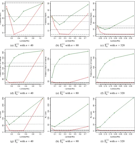
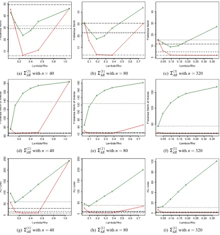
We consider two different covariance matrices. The first one is a simple auto-regressive process of order one with trivial block size equal to p=300, denoted by Σ(₀1). This is also known as a Toeplitz matrix. That is, we have Σ(_0;i1)_,j =0.9|i−j| ∀i,j∈ {1, ...,p}. The second matrix Σ(₀2) is a block-diagonal matrix with AR(1) blocks of equal block size 30_×30, and hence the block-diagonal of Σ(₀2) equals ΣBlock;i,j =0.9|i−j|, i,j∈ {1, . . . ,30}. The simulation results for the AR(1)-block

models are shown in Figure 1 and 2.

The figures show a substantial performance gain of our method compared to the GLasso in both considered covariance models. This result speaks for our method, especially because AR(1)-block models are very simple. The Space method performs about as well as Gelato, except for the Frobe-nius norm ofΣbn−Σ0. There we see an performance advantage of the Space method compared to

Gelato. We also exploit the clear advantage of thresholding in Gelato for a small sample size.

4.1.2 THERANDOMPRECISIONMATRIXMODEL

For this model we also consider two different matrices, which differ in sparsity. For the sparser matrixΘ(₀3)we set the probabilityπto 0.1. That is, we have an off diagonal entry inΘ(3)of 0.5 with probabilityπ=0.1 and an entry of 0 with probability 0.9. In the case of the second matrixΘ(₀4)we setπto 0.5 which provides us with a denser concentration matrix. The simulation results for the two performance measures are given in Figure 3 and 4.

From Figures 3 and 4 we see that GLasso performs better than Gelato with respect to_kΘbn−Θ0kF

and the Kullback Leibler divergence in both the sparse and the dense simulation setting. If we consider_kbΣn−Σ0kF, Gelato seems to keep up with GLasso to some degree. For the Space method

we have a similar situation to the one with GLasso. The Space method outperforms Gelato for

(a) Σ(₀1)with n=40 (b)Σ₀(1)with n=80 (c)Σ(₀1)with n=320

(d)Σ(₀1)with n=40 (e) Σ₀(1)with n=80 (f) Σ(₀1)with n=320

(g)Σ(₀1)with n=40 (h)Σ₀(1)with n=80 (i)Σ(₀1)with n=320

(a) Σ(_AR2)with n=40 (b)Σ_AR(2)with n=80 (c)Σ(_AR2)with n=320

(d)Σ(_AR2)with n=40 (e) Σ_AR(2)with n=80 (f) Σ(_AR2)with n=320

(g)Σ(_AR2)with n=40 (h)Σ_AR(2)with n=80 (i)Σ(_AR2)with n=320

(a) Θ(₀3)with n=40 (b)Θ₀(3)with n=80 (c)Θ(₀3)with n=320

(d)Θ(₀3)with n=40 (e) Θ₀(3)with n=80 (f) Θ(₀3)with n=320

(g)Θ(₀3)with n=40 (h)Θ₀(3)with n=80 (i)Θ(₀3)with n=320

(a) Θ(₀4)with n=40 (b)Θ₀(4)with n=80 (c)Θ(₀4)with n=320

(d)Θ(₀4)with n=40 (e) Θ₀(4)with n=80 (f) Θ(₀4)with n=320

(g)Θ(₀4)with n=40 (h)Θ₀(4)with n=80 (i)Θ(₀4)with n=320

4.1.3 THEEXPONENTIALDECAYMODEL

In this simulation setting we only have one version of the concentration matrixΘ(₀5). The entries of Θ(5)

0 are generated byθ

(5)

0,i j=exp(−2|i−j|). Thus,Σ0is a banded and sparse matrix.

Figure 5 shows the results of the simulation. We find that all three methods show equal performances in both the Frobenius norm and the Kullback Leibler divergence. This is interesting because even with a sparse approximation ofΘ0(with GLasso or Gelato), we obtain competitive performance for (inverse) covariance estimation.

4.1.4 SUMMARY

Overall we can say that the performance of the methods depend on the model. For the models Σ(1)

0 andΣ

(2)

0 the Gelato method performs best. In case of the modelsΘ

(3)

0 andΘ

(4)

0 , Gelato gets outperformed by GLasso and the Space method and for the modelΘ(₀5) none of the three methods has a clear advantage. In Figures 1 to 4, we see the advantage of Gelato with thresholding over the one without thresholding, in particular, for the simulation settings Σ(₀1), Σ₀(2) and Θ(₀3). Thus thresholding is a useful feature of Gelato.

4.2 Application to Real Data

We show two examples in this subsection.

4.2.1 ISOPRENOIDGENEPATHWAY INARABIDOBSISTHALIANA

In this example we compare the two estimators on the isoprenoid biosynthesis pathway data given in Wille et al. [2004]. Isoprenoids play various roles in plant and animal physiological processes and as intermediates in the biological synthesis of other important molecules. In plants they serve numerous biochemical functions in processes such as photosynthesis, regulation of growth and de-velopment. The data set consists of p=39 isoprenoid genes for which we have n=118 gene expression patterns under various experimental conditions. In order to compare the two techniques we compute the negative log-likelihood via 10-fold cross-validation for different values ofλ,τand ρ. In Figure 6 we plot the cross-validated negative log-likelihood against the logarithm of the av-erage number of non-zero entries (logarithm of theℓ0-norm) of the estimated concentration matrix

b

Θn. The logarithm of the ℓ0-norm reflects the sparsity of the matrix Θbn and therefore the figures

(a) Θ(₀5)with n=40 (b)Θ₀(5)with n=80 (c)Θ(₀5)with n=320

(d)Θ(₀5)with n=40 (e) Θ₀(5)with n=80 (f) Θ(₀5)with n=320

(g)Θ(₀5)with n=40 (h)Θ₀(5)with n=80 (i)Θ(₀5)with n=320

(a) isoprenoid data (b) breast cancer data

Figure 6: Plots for the isoprenoid data from arabidopsis thaliana (a) and the human breast cancer data (b). 10-fold cross-validation of negative log-likelihood against the logarithm of the average number of non-zero entries of the estimated concentration matrixΘbn. The circles

stand for the GLasso and the Gelato is displayed for various values ofτ.

4.2.2 CLINICALSTATUS OFHUMANBREASTCANCER

As a second example, we compare the two methods on the breast cancer data set from West et al. [2001]. The tumor samples were selected from the Duke Breast Cancer SPORE tissue bank. The data consists of p=7129 genes with n=49 breast tumor samples. For the analysis we use the 100 variables with the largest sample variance. As before, we compute the negative log-likelihood via 10-fold cross-validation. Figure 6 shows the results. In this real data example the interpretation of the plots is similar as for the arabidopsis data set. For dense fits, GLasso is better while Gelato has an advantage when requiring a sparse fit.

5. Conclusions

We propose and analyze the Gelato estimator. Its advantage is that it automatically yields a positive definite covariance matrixbΣn, it enjoys fast convergence rate with respect to the operator and

Frobe-nius norm ofΣbn−Σ0andΘbn−Θ0. For estimation ofΘ0, Gelato has in some settings a better rate

the selected edge setEbnwhile ensuring that we do not introduce too much bias. Our Gelato method

also addresses the bias problem inherent in the GLasso estimator since we no longer shrink the en-tries in the covariance matrix corresponding to the selected edge setEbnin the maximum likelihood

estimate, as shown in Section 3.3.

Our experimental results show that Gelato performs better than GLasso or the Space method for AR-models while the situation is reversed for some random precision matrix models; in case of an exponential decay model for the precision matrix, all methods exhibit the same performance. For Gelato, we demonstrate that thresholding is a valuable feature. We also show experimentally how one can use cross-validation for choosing the tuning parameters in regression and thresholding. Deriving theoretical results on cross-validation is not within the scope of this paper.

Acknowledgments

We thank Larry Wasserman, Liza Levina, the anonymous reviewers and the editor for helpful com-ments on this work. Shuheng Zhou thanks Bin Yu warmly for hosting her visit at UC Berkeley while she was conducting this research in Spring 2010. SZ’s research was supported in part by the Swiss National Science Foundation (SNF) Grant 20PA21-120050/1. Min Xu’s research was supported by NSF grant CCF-0625879 and AFOSR contract FA9550-09-1-0373.

Appendix A. Theoretical Analysis and Proofs

In this section, we specify some preliminary definitions. First, note that when we discuss estimating the parametersΣ0andΘ0=Σ−₀1, we always assume that

ϕmax(Σ0):=1/ϕmin(Θ0)_≤1/c<∞ and 1/ϕmax(Θ0) =ϕmin(Σ0)_≥k>0, (33)

where we assume k,c_≤1 so that c_≤1_≤1/k. (34)

It is clear that these conditions are exactly that of (A2) in Section 3 with

Mupp:=1/c and Mlow:=k,

where it is clear that forΣ0,ii=1,i=1, . . . ,p, we have the sum of p eigenvalues ofΣ0,∑_ip₌₁ϕi(Σ0) =

tr(Σ0) =p. Hence it will make sense to assume that (34) holds, since otherwise, (33) implies that

ϕmin(Σ0) =ϕmax(Σ0) =1 which is unnecessarily restrictive.

We now define parameters relating to the key notion of essential sparsity s0as explored in Cand`es and Tao [2007] and Zhou [2009, 2010a] for regression. Denote the number of zero non-diagonal entries in each row of Θ0 by si. Let s=maxi=1,...,psi denote the highest node degree

in G= (V,E0). Consider nodewise regressions as in (2), where we are given vectors of parameters

{βi

si₀≤si≤s as the smallest integer such that p

∑

j=1,j6=i

min((βi

j)2,λ2Var(Vi))≤si0λ2Var(Vi),whereλ=

p

2 log p/n, (35)

where si₀denotes si_0,nas defined in (7).

Definition 8 (Bounded degree parameters.) The size of the node degree sifor each node i is upper bounded by an integer s<p. For si₀as in (35), define

s0 := max

i=1,...,ps i

0≤s and S0,n :=

∑

i=1,...,p

si₀, (36)

where S0,n is exactly the same as in (8), although we now drop subscript n from si0,n in order to simplify our notation.

We now define the following parameters related toΣ0. For an integer m_≤p, we define the smallest and largest m-sparse eigenvalues ofΣ0as follows:

p

ρmin(m) := min

t6=0;m−sparse Σ10/2t

₂

kt_k2 ,

p

ρmax(m) := max

t6=0;m−sparse Σ10/2t

₂

kt_k2 .

Definition 9 (Restricted eigenvalue condition RE(s0,k0,Σ0)). For some integer 1≤s0<p and a

positive number k0, the following condition holds for allυ6=0, 1

K(s0,k0,Σ0)

:= min

J⊆{1,...,p}, |J_|≤s0

min

kυJck1≤k0kυJk1

Σ10/2υ

2

kυJk2

>0, (37)

whereυJ represents the subvector ofυ∈Rpconfined to a subset J of{1, . . . ,p}.

When s0 and k0 become smaller, this condition is easier to satisfy. When we only aim to estimate the graphical structure E0 itself, the global conditions (33) need not hold in general. Hence up till Section D, we only need to assume thatΣ0satisfies (37) for s0as in (35), and the sparse eigenvalue ρmin(s)>0. In order of estimate the covariance matrixΣ0, we do assume that (33) holds, which guarantees that the RE condition always holds on Σ0, andρmax(m),ρmin(m) are upper and lower bounded by some constants for all m_≤p. We continue to adopt parameters such as K,ρmax(s), and ρmax(3s0)for the purpose of defining constants that are reasonable tight under condition (33). In general, one can think of

ρmax(max(3s0,s))≪1/c<∞ and K2(s0,k0,Σ0)≪1/k<∞, for c,k as in (33) when s0is small.

Roughly speaking, for two variables Xi,Xj as in (1) such that their corresponding entry in Θ0=

(θ0,i j)satisfies:θ0,i j<λ

p_θ0

,ii, whereλ=

p

we aim to keep≍si₀edges for node i,i=1, . . . ,p. For a givenΘ0, as the sample size n increases, we are able to select edges with smaller coefficientθ0,i j. In fact it holds that

|θ0,i j|<λ

p

θ0,iiwhich is equivalent to|βij|<λσVi, for all j≥s i

0+1+Ii≤si

0+1, (38)

whereI_{{·} is the indicator function, if we order the regression coefficients as follows:}

|βi

1| ≥ |βi2|...≥ |βii₋1| ≥ |βii+1|....≥ |βip|, in view of (2), which is the same as if we order for row i ofΘ0,

|θ0,i1| ≥ |θ0,i,2|...≥ |θ0,i,i−1| ≥ |θ0,i,i+1|....≥ |θ0,i,p|.

This has been shown by Cand`es and Tao [2007]; See also Zhou [2010a].

A.1 Concentration Bounds for the Random Design

For the random design X generated by (15), letΣ0,ii=1 for all i. In preparation for showing the

oracle results of Lasso in Theorem 33, we first state some concentration bounds on X . Define for some 0<θ<1

F

(θ):=X :_∀j=1, . . . ,p,1₋θ_≤Xj

₂/√n_≤1+θ , (39) where X1, . . . ,Xpare the column vectors of the n×p design matrix X . When all columns of X have

an Euclidean norm close to√n as in (39) , it makes sense to discuss the RE condition in the form of (40) as formulated by Bickel et al. [2009]. For the integer 1_≤s0<p as defined in (35) and a positive number k0, RE(s0,k0,X)requires that the following holds for allυ6=0,

1 K(s0,k0,X)

△

= min

J⊂{1,...,p}, |J|≤s0

min

kυJck1≤k0kυJk1

kXυ_k2 √_n

kυJk2

>0. (40)

The parameter k0>0 is understood to be the same quantity throughout our discussion. The fol-lowing event

R

provides an upper bound on K(s0,k0,X) for a given k0 >0 when Σ0 satisfies

RE(s0,k0,Σ0)condition:

R

(θ):=

X : RE(s0,k0,X) holds with 0<K(s0,k0,X)≤

K(s0,k0,Σ0) 1₋θ

.

For some integer m_≤p, we define the smallest and largest m-sparse eigenvalues of X to be

Λmin(m) := min

υ6=0;m−sparse kXυk 2

2/(nkυk 2 2) and Λmax(m) := max

υ6=0;m−sparsekXυk 2

2/(nkυk 2 2), upon which we define the following event:

M

(θ):=_{X : (41) holds_∀m_≤max(s,(k0+1)s0)},for which

Formally, we consider the set of random designs that satisfy all events as defined, for some 0<θ<1. Theorem 10 shows concentration results that we need for the present work, which follows from Theorem 1.6 in Zhou [2010b] and Theorem 3.2 in Rudelson and Zhou [2011].

Theorem 10 Let 0<θ<1. Let ρmin(s)>0, where s< p is the maximum node-degree in G. Suppose RE(s0,4,Σ0)holds for s0as in (36), whereΣ0,ii=1 for i=1, . . . ,p.

Let f(s0) =min(4s0ρmax(s0)log(5ep/s0),s0log p). Let c,α,c′ >0 be some absolute constants.

Then, for a random design X as generated by (15), we have

P₍

X

):=P₍

R

(θ)_∩

F

(θ)_∩

M

(θ))_≥1₋3 exp(₋cθ2n/α4)

as long as the sample size satisfies

n>max

9c′α4

θ2 max 36K 2_(s

0,4,Σ0)f(s0),log p, 80sα4

θ2 log

5ep sθ

. (42)

Remark 11 We note that the constraint s<p/2, which has appeared in Zhou [2010b, Theorem 1.6] is unnecessary. Under a stronger RE condition onΣ0, a tighter bound on the sample size n, which is independent ofρmax(s0), is given in Rudelson and Zhou [2011] in order to guarantee

R

(θ). We

do not pursue this optimization here as we assume thatρmax(s0)is a bounded constant throughout

this paper. We emphasize that we only need the first term in (42) in order to obtain

F

(θ)and

R

(θ); The second term is used to bound sparse eigenvalues of order s.

A.2 Definitions Of Other Various Events

Under (A1) as in Section 3, excluding event

X

c _{as bounded in Theorem 10 and events}

_C

_a,

_X

0 to be defined in this subsection, we can then proceed to treat X_∈

X

_∩

C

_a as a deterministic design in regression and thresholding, for which

R

(θ)_∩

M

(θ)_∩

F

(θ) holds with

C

_a, We then make use of event

X

0in the MLE refitting stage for bounding the Frobenius norm. We now define two types of correlations events

C

_aand

X

₀.

A.2.1 CORRELATIONBOUNDS ONXj ANDVi

In this section, we first bound the maximum correlation between pairs of random vectors(Vi,Xj),

for all i,j where i₆= j, each of which corresponds to a pair of variables (Vi,Xj) as defined in (2)

and (3). Here we use Xj and Vi, for all i,j, to denote both random vectors and their corresponding

variables.

Let us defineσVj :=

p

Var(Vj)≥v>0 as a shorthand. Let Vj′:=Vj/σVj,j=1, . . . ,p be a standard

normal random variable. Let us now define for all j,k₆= j,

Zjk=

1 nhV

′ j,Xki=

1 n

n

∑

i=1

where for all i=1, . . . ,n v′_j,i,xk,i,∀j,k6= j are independent standard normal random variables. For

some a_≥6, let event

C

a:=

max

j,k |Zjk|< √

1+ap(2 log p)/n where a_≥6

.

A.2.2 BOUNDS ONPAIRWISECORRELATIONS INCOLUMNSOFX

LetΣ0:= (σ0,i j), where we denote σ0,ii:=σ2i. Denote by ∆=XTX/n−Σ0. Consider for some

constant C3>4 p

5/3,

X

₀:=

max

j,k |∆jk|<C3σiσj

p

log max_{p,n_}/n<1/2

. (43)

We first state Lemma 12, which is used for bounding a type of correlation events across all regres-sions; see proof of Theorem 15. It is also clear that event

C

_ais equivalent to the event to be defined in (44). Lemma 12 also justifies the choice ofλn in nodewise regressions (cf. Theorem 15). We

then bound event

X

₀in Lemma 13. Both proofs appear in Section A.3.

Lemma 12 Suppose that p<en/4C22_{. Then with probability at least 1}−₁/_p2_{, we have} ∀j₆=k,

1

nhVj,Xki

≤σVj

√

1+ap(2 log p)/n, (44)

whereσVj =

p

Var(Vj)and a≥6. HenceP(

C

a)≥1−1/p2.

Lemma 13 For a random design X as in (1) with Σ0,j j=1,∀j∈ {1, . . . ,p}, and for p<en/4C 2 3,

where C3>4 p

5/3, we have

P₍

X

₀)_≥1₋1/max_{n,p_}2.

We note that the upper bounds on p in Lemma 12 and 13 clearly hold given (A1). For the rest of the paper, we prove Theorem 15 in Section B for nodewise regressions. We proceed to derive bounds on selecting an edge set E in Section C. We then derive various bounds on the maximum likelihood estimator given E in Theorem 19- 21 in Section D, where we also prove Theorem 1. Next, we prove Lemma 12 and 13 in Section A.3.

A.3 Proof of Lemma 12 and 13

We first state the following large inequality bound on products of correlated normal random vari-ables.

Lemma 14 Zhou et al., 2008, Lemma 38 Given a set of identical independent random variables

Y1, . . . ,Yn∼Y , where Y =x1x2, with x1,x2∼N(0,1) andσ12=ρ12 withρ12≤1 being their

cor-relation coefficient. Let us now define Q= 1

n∑ n