Efficient Margin Maximizing with Boosting
∗Gunnar R¨atsch [email protected]
Friedrich Miescher Laboratory of the Max Planck Society Spemannstrasse 35
72076 T¨ubingen, Germany
Manfred K. Warmuth [email protected]
University of California at Santa Cruz Santa Cruz, CA 95060, USA
Editor: John Shawe-Taylor
Abstract
AdaBoost produces a linear combination of base hypotheses and predicts with the sign of this linear combination. The linear combination may be viewed as a hyperplane in feature space where the base hypotheses form the features. It has been observed that the generalization error of the algo-rithm continues to improve even after all examples are on the correct side of the current hyperplane. The improvement is attributed to the experimental observation that the distances (margins) of the examples to the separating hyperplane are increasing even after all examples are on the correct side. We introduce a new version of AdaBoost, called AdaBoost∗ν, that explicitly maximizes the minimum margin of the examples up to a given precision. The algorithm incorporates a current es-timate of the achievable margin into its calculation of the linear coefficients of the base hypotheses. The bound on the number of iterations needed by the new algorithms is the same as the number needed by a known version of AdaBoost that must have an explicit estimate of the achievable mar-gin as a parameter. We also illustrate experimentally that our algorithm requires considerably fewer iterations than other algorithms that aim to maximize the margin.
1. Introduction
Boosting algorithms are greedy methods for forming linear combinations of base hypotheses. In the most common scenario the algorithm is given a fixed set of labeled training examples and in each iteration updates a distribution on these examples (i.e. a set of non-negative weights that sum to one). It then is given a base hypothesis whose weighted error (probability of wrong classification) is slightly below 50%. This base hypothesis is used to update the distribution on the examples: The algorithm increases the weights of those examples that were wrongly classified by the base hypothesis. At the end of each stage the base hypothesis is added to the linear combination, and the sign of this linear combination forms the current hypothesis of the boosting algorithm.
The most well known boosting algorithm is AdaBoost (Freund and Schapire, 1997). It is ”adap-tive” in that the linear coefficient of the base hypothesis depends on the weighted error of the base hypothesis at the time when the base hypothesis was added to the linear combination. AdaBoost has two interesting properties. First, along with earlier boosting algorithms (Schapire, 1992; Freund, 1995), its training error has the following exponential convergence property: if the weighted train-ing error of the t-th base hypothesis isεt = 12−12γt, then an upper bound on the training error of
the signed linear combination is reduced by a factor of 1−1
2γ2t at stage t. Second, it has been
ob-served experimentally that AdaBoost continues to “learn” even after the training error of the signed linear combination is zero (Schapire et al., 1998). That is, in experiments the generalization error continues to improve. The signed linear combination can be viewed as a homogeneous hyperplane in a feature space, where each base hypothesis represents one feature or dimension. We define the margin of an example as a signed distance to the hyperplane times its±label (See Section 2 and Appendix A for precise definitions). As soon as the training error is zero, the examples are on the right side and all have positive margin. It has also been observed that the margins of the examples continue to increase even after the training error is zero. There are theoretical bounds on the gen-eralization error of linear classifiers (e.g. Schapire et al., 1998; Breiman, 1999; Koltchinskii et al., 2001) that improve with the margin of the classifier, which is defined as the size of the minimum margin of the examples. Thus the fact that the margins improve experimentally seems to explain why AdaBoost still learns after the training error is zero.
There is one flaw in this argument: AdaBoost has not been proven to maximize the margin of the final hypothesis. We demonstrate this experimentally in Section 5. Moreover, Rudin et al. (2004a, 2005) recently showed that there are cases where AdaBoost provably does not maximize the margin. Breiman (1999) proposed a modified algorithm – called Arc-GV (Arcing-Game Value) – suitable for this task and showed that it asymptotically maximizes the margin. Similar results are shown in Grove and Schuurmans (1998) and Bennett et al. (2000). In this paper we present an algorithm that produces a final hypothesis with margin at leastρ∗−ν, whereρ∗is the unknown maximum margin achievable by any convex combination of base hypotheses andνa precision parameter.
If we know ρ∗, then a linear combination with margin at least ρ∗−νcan be found by a pa-rameterized version of AdaBoost called AdaBoostρ (cf. R¨atsch et al. (2001); R¨atsch and Warmuth (2002)): When the parameter ρof AdaBoostρ is set toρ∗−ν, then after 2 ln N
ν2 iterations, where
N is the number of examples, the margin of the produced linear combination is guaranteed to be at least ρ∗−ν. The case when ρ∗ is not known is more difficult. In a preliminary conference paper (R¨atsch and Warmuth, 2002) we used AdaBoostρiteratively in a binary search like fashion: log2(2/ν)calls to AdaBoostρare guaranteed to produce a margin at leastρ∗−ν. All but the last call to AdaBoostρare used to find a suitable value of the parameterρand in the last call this parameter is used to create the final linear combination in at most 2 ln Nν2 iterations.
In this paper we greatly simplify our answer for the case when ρ∗ is unknown. We have a new one pass algorithm called AdaBoost∗ν that produces a linear combination with margin at least ρ∗−νafter 2 ln N
ν2 iterations. Note that this is the same guarantee we had on the number of iterations
of AdaBoostρ when it used the theoretically optimal parameter ρ=ρ∗−ν. The new algorithm AdaBoost∗νuses the parameterνand a current estimate of the achievable margin in the computation of the linear coefficients of the base learners.
a final hypothesis with margin at leastρ∗/2 ifρ∗>0 and if subtle conditions on the chosen base hypotheses are satisfied (cf. Corollary 5).
Recently other versions of AdaBoost have been published that are guaranteed to produce a lin-ear combination of margin at least ρ∗−ν after Ω(ν−3) iterations (Rudin et al., 2004c,b). Even though these algorithms have weaker iteration bounds than AdaBoost∗ν, they were reported to per-form better experimentally (Rudin et al., 2004c,a). We briefly compare AdaBoost∗ν to these more recent algorithms and show that the better empirical performance was due to the wrong choice ofν. The original AdaBoost was designed to find a final hypothesis of margin at least zero. Our algorithm maximizes the margin for all values ofρ∗. This includes the inseparable case (i.e.ρ∗<0), where one minimizes the overlap between the two classes. In this case AdaBoost runs forever without necessarily increasing the margin. Our algorithm is also useful when the base hypotheses given to the Boosting algorithm are strong in the sense that they already separate the data and have margin greater than zero, but less than one. In this case 0<ρ∗ <1 and AdaBoost aborts immediately because the linear coefficients of such hypotheses become unbounded. In contrast, our new algorithm also maximizes the margin when presented with strong learners.
The big advantage of this algorithm is an absolute bound on the number of iterations: After 2 ln N
ν2 iterations AdaBoost∗ν is guaranteed to produce a hypothesis with margin at leastρ∗−ν. Our
algorithm is applicable in sophisticated settings where the number of hypotheses may be infinite. In Appendix B we use AdaBoost∗νto learn a convex combination of support vector kernels and show that the same guarantees hold on the number of iterations of the algorithm.
The paper is structured as follows: Section 2 introduces some basic notation and in Section 3 we first describe AdaBoostρwhich requires a lower boundρof the maximum marginρ∗as a parameter. Then we present our new algorithm AdaBoost∗ν, which is similar to AdaBoostρ, but continuously adaptsρbased on a precision parameterν. Up to this point we stay at a high level of presentation with the goal of making our algorithms accessible to the quick reader. In Section 4 we introduce more notation and give a detailed analysis of both algorithms. First, we prove that if the weighted training error of the t-th base hypothesis isεt = 12−12γt, then an upper bound on the fraction of
examples with margin smaller thanρis reduced by a factor of 1−1
2(ρ−γt)
2at stage t of AdaBoost ρ (cf. Section 4.2) (A slightly improved factor is shown for the case whenρ>0). However, to achieve a large margin one needs to assume that the guessρis smaller thanρ∗. For the latter case we prove an exponential convergence rate of AdaBoostρ. Then we discuss a method for automatically tuning ρdepending on the errors of the base hypotheses and a precision parameterν. We show that after roughly 2 ln Nν2 iterations our new one-pass algorithm AdaBoost∗ν is guaranteed to produce a linear
combination with margin at leastρ∗−ν. This strengthens the results of our preliminary conference paper (R¨atsch and Warmuth, 2002), which had an additional log2(2/ν)factor in the total number times the weak learner is called and much higher constants. In Section 5, we compare the algorithms experimentally and discuss heuristics for tuningνin Section 5.2. Finally we briefly summarize and discuss our results in the Conclusion Section.
2. Preliminaries and Basic Notation
We consider the standard two-class supervised machine learning problem: Given a set of N i.i.d. training examples(xn,yn), n=1, . . . ,N, with xn∈
X
and yn∈Y
:={−1,+1}, we would like toIn the case of ensemble learning (like boosting), there is a fixed underlying set of base hypothe-ses
H
:={h|h :X
→[−1,1]}from which the ensemble is built. For now we only assume thatH
is finite, but we will show in Section 4.5 that this assumption can be dropped in most cases and that all of the following analysis also applies to the case of infinite hypothesis sets.
Boosting algorithms iteratively form non-negative linear combinations of hypotheses from
H
. In each iteration t, a base hypothesis ht∈H
with a non-negative coefficientαt is added to the linearcombination. We denote the combined hypothesis as follows (Note that we normalized the weights):
˜
fα(x) =sign fα(x), where fα(x) = T
∑
t=1 αt
∑T r=tαr
ht(x),ht(x)∈
H
,andαt ≥0 .The “black box” that selects the base hypothesis in each iteration is called the weak learner. For AdaBoost, it has been shown that if the weak learner is guaranteed to select base hypotheses of weighted error slightly below 50%, then the combined hypothesis is consistent with the training set in a small number of iterations (Freund and Schapire, 1997). We will discuss bounds on the number of iterations in detail in Section 4. Since at most one new base hypothesis is added in each iteration, the size of the final hypothesis is bounded by the number of iterations. These bounds are important because the sample size bounds provable in the PAC model grow with the size of the final hypothesis (Schapire, 1992; Freund, 1995).
In more recent research (Schapire et al., 1998) it was also shown that a bound on the general-ization error decreases with the size of the margin of the final hypothesis f . The margin of a single example(xn,yn)w.r.t. f is defined as ynfα(xn). Thus the margin quantifies by how far this example
is on the ynside of the hyperplane ˜f . In Appendix A we clarify how the margin of an example is
re-lated to its`∞-distance to the hyperplane with normalα. The margin of the combined hypothesis f is the minimum margin of all N examples. The goal of this paper is to find a small non-negative linear combination of base hypotheses from
H
with margin close to the maximum achievable margin.The following table gives some of the main notations that will be used throughout this paper:
Symbol Description
n,N index and number of examples
m,M index and number of hypotheses if finite t,T index and number of iterations
X
input spaceY
label space{±1}(x,y) an example and its label
H
,hm set of base hypotheses and the m-th elementα hypothesis weight vector d weighting on the training set
I(·) the indicator function: I(true) =1 and I(f alse) =0 ρ the margin parameter of AdaBoostρ
{ρt} the sequence of margin parameters of AdaBoost{ρt}
ρ∗ the maximum margin ˆ
ρt margin in the t-th iteration
ν the accuracy parameter of AdaBoost∗ν ε weighted classification error
Symbol Description
γ an arbitrary edge threshold γt the edge of the t-th hypothesis
3. AdaBoostρ and AdaBoost∗ν
The original AdaBoost was designed to find a consistent hypothesis ˜f which is defined as a signed linear combination f with margin greater zero. We start with a slight modification of AdaBoost, which finds (if possible) a linear combination of base learners with marginρ, whereρis a parameter (cf. Algorithm 1).1 We call this algorithm AdaBoostρ, as it naturally generalizes AdaBoost for the case when the target margin isρ. The original AdaBoost algorithm now becomes AdaBoost0.
Algorithm 1: – The AdaBoostρalgorithm – with margin parameterρ 1. Input: S=h(x1,y1), . . . ,(xN,yN)i, No. of IterationsT, margin targetρ
2. Initialize: dn1=N1 for alln=1. . .N
3. Do for t=1, . . . ,T,
(a) Train classifier on{S,dt}and obtain hypothesish
t : x7→[−1,1] (b) Calculate the edgeγt ofht:γt=
N
∑
n=1
dntynht(xn)
(c) if|γt|=1,thenα1=sign(γt),h1=ht,T =1; break (d) Setαt =
1 2ln
1+γt
1−γt
−1 2ln
1+ρ
1−ρ
(e) Update weights:dtn+1=d t
nexp(−αtynht(xn))
Zt
,
whereZt=∑Nn=1dntexp(−αtynht(xn)) 4. Output: fα(x) =
T
∑
t=1 αt
∑T r=1αr
ht(x)
The algorithm AdaBoostρ was already known as unnormalized Arcing (Breiman, 1999) or AdaBoost-type Algorithm (R¨atsch et al., 2001). Moreover, it is related to algorithms proposed in Freund and Schapire (1999) and Zhang (2002). The only difference from AdaBoost is the choice of the hypothesis coefficientsαt: An additional term−12ln11−ρ+ρ appears in the expression for the
hy-pothesis coefficientαt. This term vanishes whenρ=0. The parameterρcan be seen as a guess of
the maximum marginρ∗. Ifρis chosen properly (slightly belowρ∗), then AdaBoostρwill converge exponentially fast to a combined hypothesis with nearly the maximum margin. See Section 4.2 for details.
The following example illustrates how AdaBoostρworks. Assume the weak learner returns the constant hypothesis ht(x)≡1. The weighted error of this hypothesis is the sum of all negative
weights, i.e.εt=∑yn=−1d
t
nand its edge isγt=1−2εt. The coefficientαt is chosen so that the edge
of ht with respect to the new distribution is exactlyρ(instead of 0 as for the original AdaBoost).
More precisely, the given choice ofαtassures that this edge isρonly for±1-valued base hypotheses.
For a more general base hypothesis ht with continuous range[−1,+1], choosingαt such that
Zt as a function ofαt is minimized, guarantees that the edge of ht with respect to the distribution dt+1 is ρ. See Schapire and Singer (1999) for a similar discussion. Choosingαt as in step 3 (d)
approximately minimizes Zt when the range of ht is[−1,+1].
In Kivinen and Warmuth (1999) and Lafferty (1999), the standard boosting algorithms are in-terpreted as approximate solutions to the following optimization problem: choose a distribution d of maximum entropy subject to the constraints that the edges of the previous hypotheses are equal to zero. In this paper we use the inequality constraints that the edges of the previous hypotheses are at most ρ. Theαt’s function as Lagrange multipliers for these inequality constraints. Since
g(x) =1 2ln
1+x
1−x is an increasing function,
αt=
1 2ln
1+γt
1−γt
−1 2ln
1+ρ
1−ρ ≥ 0 iff γt≥ρ . (1)
Notice that whenρ=0, adding ht or−ht leads to the same distribution dt+1. This symmetry is
broken forρ6=0.
Since one does not know the value of the optimum marginρ∗is not known beforehand, one also needs to find ρ∗. In R¨atsch and Warmuth (2002) we presented the Marginal AdaBoost algorithm which constructs a sequence {ρr}Rr=1 converging to ρ∗. A fast way to find a real value up to a certain accuracyνin the interval[−1,1]is a binary search since one needs only log2(2/ν)steps.2 Thus the previous Marginal AdaBoost algorithm uses AdaBoostρr (Algorithm 1) to decide whether
the current guessρris larger or smaller thanρ∗. Depending on the outcome,ρr can be chosen so
that the region of uncertainty forρ∗ is roughly cut in half. However, in the previous algorithm all but the last of the log2(2/ν)
In this paper we propose a different algorithm, called AdaBoost∗ν. Here ν>0 is a precision parameter. The algorithm finds a non-negative linear combination with margin at leastρ∗−ν. Like Arc-GV (Breiman, 1999), the new algorithm essentially runs AdaBoostρonce but instead of using a fixed margin estimate ρ, it updates ρ in an appropriate way. We shall show iteration bounds for our algorithm AdaBoost∗ν which are not known for Arc-GV. The latter algorithm produces an essentially3 monotonically increasing sequence of margin estimates, while in AdaBoost∗ν we use a monotonically decreasing sequence. The improved sequence of estimates is based on two new theoretical insights, which will be developed in the next section.
We will show that the number of iterations required by the new one-pass AdaBoost∗νalgorithm (see Algorithm 2 for pseudo-code) is at most 2 ln Nν2 . This equals the iteration bound for the best
algorithm we know of for the case whenρ∗ is known and we seek a linear combination of margin at leastρ∗−ν: AdaBoostρwith parameterρ=ρ∗−ν. The iteration bound for the new algorithm is the same as the iteration bound for the last call to AdaBoostρof the previous Marginal AdaBoost algorithm.
2. If one knows thatρ∗∈[a,b], one needs only log2((b−a)/ν)steps.
Algorithm 2: – The AdaBoost∗νalgorithm – with accuracy parameterν 1. Input: S=h(x1,y1), . . . ,(xN,yN)i, No. of IterationsT, desired accuracyν 2. Initialize: dn1=1/Nfor alln=1. . .N
3. Do for t=1, . . . ,T,
(a) Train classifier on{S,dt}and obtain hypothesish
t : x7→[−1,1] (b) Calculate the edgeγt ofht:γt=
N
∑
n=1
dntynht(xn)
(c) if|γt|=1,thenα1=sign(γt),h1=ht,T =1; break (d) γtmin= min
r=1,...,tγr; ρt =γ
min
t −ν
(e) Setαt =
1 2ln
1+γt
1−γt
−1 2ln
1+ρt
1−ρt
(f) Update weights:dtn+1=d t
nexp(−αtynht(xn))
Zt
,
whereZt=∑Nn=1dntexp(−αtynht(xn)) 4. Output: fα(x) =
T
∑
t=1 αt
∑T r=1αr
ht(x)
4. Detailed Analysis
In this section we are going to analyze the algorithms in detail. We start by showing the relationship between optimal edges and margins, prove and illustrate the convergence properties of AdaBoostρ and finally prove the convergence of AdaBoost∗ν.
4.1 Weak learning and margins
The standard assumption made on the weak learning algorithm for the PAC analysis of Boosting algorithm is that the weak learner returns a hypothesis h from a fixed set
H
that is slightly better than random guessing. That is, that the error rateε is consistently smaller than 12. Note that the error rate of 12 could easily be reached by a fair coin, assuming both classes have the same prior probabilities. More formally, the error ε of a±1 valued hypothesis is defined as the fraction of examples that are misclassified. In Boosting this is extended to weighted example sets and the error is defined asεh(d) = N
∑
n=1
dnI(yn6=h(xn)),
where h is the hypothesis returned by the weak learner and I is the indicator function with I(true) =1 and I(false) =0. The distribution d= (d1, . . . ,dN)of the examples is such that dn≥0 and∑Nn=1dn=
When the range of a hypothesis h is the entire interval[−1,+1], then the edgeγh(d) =∑Nn=1dnynh(xn)
is a more convenient quantity for measuring the quality of h. This edge is an affine transformation of the error for the case when h has range±1:εh(d) =12−12γh(d)andεh(d)≤21 iffγh(d)≥0.
Recall from Section 2 that the margin of a given example(xn,yn)is defined as ynfα(xn). Also
recall that
H
is the set from which the weak learner chooses its base hypotheses. Assume for a moment thatH
is finite. If we combine all hypotheses fromH
, then the following well-known the-orem establishes the connection between margins and edges (first seen in connection with Boosting in Freund and Schapire, 1996; Breiman, 1999):4Theorem 1 (Min-Max-Theorem, von Neumann (1928))
γ∗:=min
d m=max1,...,M N
∑
n=1
dnynhm(xn) = max
α n=min1,...,Nyn M
∑
m=1
αmhm(xn) =:ρ∗, (2)
where d∈
P
N,α∈P
Mand M=|H
|. HereP
kdenotes the k-dimensional probability simplex.Thus, the minimum edgeγ∗that can be achieved over all possible distributions d of the training set is equal to the maximum marginρ∗of any linear combination of hypotheses from
H
. Also, for any non-optimal distributions d and and hypothesis weightsαwe always havemax
h∈H γh(d) > γ
∗=ρ∗ > min
n=1,...,Nynfα(xn).
In particular, if the weak learning algorithm is guaranteed to return a hypothesis with edge at least γfor any distribution on the examples, thenγ∗≥γand by the above duality there exists a combined hypothesis with margin at leastγ. Ifγis equal to its upper boundγ∗then there exists a combined hypothesis with margin exactlyγ=ρ∗ that only uses hypotheses that are actually returned by the weak learner in response to certain distributions on the examples.
From this discussion we can derive a sufficient condition on the weak learning algorithm to reach the maximum margin (for the case when
H
finite). If the weak learner returns hypotheses whose edges are at leastγ∗, then there exists a linear combination of these hypotheses that attains a margin γ∗=ρ∗. We will prove later that our AdaBoost∗ν algorithm efficiently finds a linear combination with margin close toρ∗(cf. Theorem 6).
Constraining the edges of the previous hypotheses to equal zero (as done in the totally corrective algorithm of Kivinen and Warmuth (1999)) leads to a problem if there is no solution satisfying these constraints. At the end of trial t, the set of previous hypotheses is
H
t ={h1, . . . ,ht}and the totallycorrective algorithm finds a distribution such thatγh(d) =0, for all h∈
H
t. Because of the aboveduality and the fact that
H
t⊆H
, γ∗t :=min d maxh∈Ht
γh(d) ≤ γ∗=ρ∗ .
The non-decreasing sequence(γ∗
t) converges toρ∗ from below. If ρ∗>0, then the equality
con-straints on the edges are not satisfiable as soon asγ∗t >0.
In contrast our new algorithm AdaBoost∗ν is motivated by a system of inequality constraints γh(d)≤ρ, for h∈Ht, whereρis adapted. Again, ifρ<ρ∗, then the system of inequalities with this
ˆ
ρmay not have a solution (and the Lagrange multipliers may diverge to infinity). In AdaBoost∗νwe start withρlarge and decrease it when necessary. As we shall see, the algorithm maintains a margin parameterρthat is always at leastρ∗−ν.
4.2 Convergence properties of AdaBoostρ
Let AdaBoost{ρt}denote the version of AdaBoostρthat uses a time varying margin parameterρt at
iteration t. Thus in step 3 (d) of the algorithm,ρis replaced byρt. This extension will be necessary
for the later analysis of AdaBoost∗ν. The sequences{ρt}tT=1 might be specified while running the algorithm. For instance, in the algorithm Arc-GV, Breiman (1999) choosesρtas min
n=1,...,Nynfαt−1(xn).
Breiman (1999) showed that Arc-GV asymptotically converges to the maximum margin (see dis-cussion in next section). In the following we answer the question how to best choose the sequence {ρt}so as to optimize bounds on the fraction of examples which have a margin at mostρ.
Lemma 2 For anyρ∈[−1,1], the final hypothesis fα of AdaBoost{ρt} satisfies the following in-equality:
1 N
N
∑
n=1
I(ynfα(xn)≤ρ) ≤ T
∏
t=1 Zt ! exp ( T
∑
t=1 ραt
)
= T
∏
t=1
exp{ραt+ln Zt} (3)
where Zt =∑Nn=1dtnexp(−αtynht(xn))andαt =12ln1−γ1+γtt−12ln11−ρ+ρtt.
The proof directly follows from a simple extension of Theorem 1 in Schapire and Singer (1999) (see also Schapire et al. (1998)).
We now use a lemma from R¨atsch et al. (2001) to upper bound the right hand side (rhs) of the above inequality:
Lemma 3 Letγt be the edge of ht in the t-th iteration of AdaBoost{ρt}. Assume−1≤ρt ≤γt. Then
for allρ∈[−1,1],
exp{ραt+ln Zt} ≤exp
−1+ρ
2 ln
1+ρt
1+γt
−1−ρ 2 ln
1−ρt
1−γt
. (4)
Note that this generalizes Theorem 5 of (Freund and Schapire, 1997) to the case when the target margin is not zero.
AdaBoost{ρt} makes progress, if the rhs of (4) is smaller than one. Suppose we would like to reach a marginρon all training examples, where we obviously need to assumeρ≤ρ∗. We can then ask which sequence of{ρt}Tt=1one should use to find such combined hypothesis in as few iterations as possible. The rhs of (4) can be rewritten as
exp(∆2(ρ,ρt)−∆2(ρ,γt)),
where∆2(a,b):=1+2aln11++ba+1−2aln1−1−abdenotes the binary relative entropy between a,b∈[−1,1]. Therefore the rhs of (4) is minimized forρt =ρ(independent ofγt) and one should always use this
constant choice.
This means that when ρt =ρ then the rhs of (4) is reduced by a factor of exp(−∆2(ρ,γt)),
which can be upper bounded by inspecting the Taylor expansion atγt =ρand noticing that when
0≤ρ<γt, all terms of order three and higher are negative:
exp(−∆2(ρ,γt))<1−
1 2
(ρ−γt)2
The denominator 1−ρ2speeds up the convergence whenρ0. Notice that whenρ=0, then we recover the original AdaBoost bound.
Now we determine an upper bound on the number of iterations needed by AdaBoostρfor achiev-ing a margin ofρon all examples, given that the maximum margin isρ∗:
Corollary 4 Assume the weak learner always returns a base hypothesis with an edgeγt ≥ρ∗. If
0≤ρ≤ρ∗−ν,ν>0, then AdaBoostρwill converge to a solution with margin at least ρon all examples in at most 2 ln Nν(1−ρ2 2) iterations.
Proof By Lemma 2 and (4), (5):
1 N
N
∑
n=1
I(ynf(xn)≤ρ)< T
∏
t=1
1−1 2
(ρ−γt)2
1−ρ2
≤
1−1 2
ν2 1−ρ2
T .
The margin is at leastρfor all examples, if the rhs is smaller than N1; hence after at most ln N
−ln
1−121−ρν22
≤
2 ln N(1−ρ2) ν2
iterations, which proves the statement.
Whenρ<0, then inequality (5) can be replaced with the following weaker inequality which holds for all distinctρ,γt∈[−1,1]:
exp(−∆2(ρ,γt))<exp
−1
2(ρ−γt) 2
. (6)
This leads to the same bound as in the above corollary except that the factor(1−ρ2) is omitted. Thus whenρ<0, the bound on the number of iterations becomes 2 ln Nν2 (R¨atsch, 2001, page 25). 4.3 Asymptotic Margin of AdaBoostρ
With the methods shown so far we can determine the asymptotic value of margin of the hypothesis produced by the original AdaBoost algorithm. First, we state a lower bound on the margin that is achieved by AdaBoostρ. There is a gap between this lower bound and the upper bound of Theorem 1. In a second part we consider an experiment that shows that depending on some subtle properties of the weak learner, the margin of combined hypotheses generated by AdaBoost can converge to quite different values (while the maximum margin is kept constant). We observe that the previously lower bound on the margin is quite tight in empirical cases.
As long as each factor in the rhs of Eq. (3) is smaller than 1, the bound decreases. If the factor is at most 1−µ and µ>0, then the rhs converges exponentially fast to zero. The following corollary considers the asymptotic case and gives a lower bound on the margin.
Corollary 5 (R¨atsch (2001)) Assume AdaBoostρgenerates hypothesis h1,h2, . . .with edgesγ1,γ2, . . .and coefficientsα1,α2, . . .. Letγmin=inft=1,2,...γt and assumeγmin>ρ. Furthermore, let
ˆ
ρt = min n=1,...,N
yn∑tr=1αrhr(xn)
be the achieved margin in the t-th iteration and ˆρ=supt=1,2,...ρˆt. Then the margin ˆρof the combined
hypothesis is bounded from below by
ˆ
ρ≥ln(1−ρ
2)−ln(1−(γmin)2) ln
1+γmin
1−γmin
−ln
1+ρ
1−ρ
. (7)
From (7) one can understand the interaction betweenρandγmin: If the difference betweenγmin andρis small, then the rhs of (7) is small. Thus, ifρwithρ≤γminis large, then ˆρmust be large, i.e. choosing a largerρresults in a larger margin on the training examples. A Taylor expansion of the rhs of (7) shows that the margin is lower bounded byγmin2+ρ. This known lower bound (Breiman, 1999, Theorem 7.2) is greater thanρifγmin>ρ.
In Section 4.1 we reasoned thatγmin≤ρ∗. If the parameter AdaBoost
ρis chosen too small, then we guarantee only that the margin of the produced linear combination converges asymptotically to a value at belowρ∗. In the original formulation of AdaBoost we haveρ=0 and we guarantee only that AdaBoost0achieves a margin of at least γ
min+ρ
2 =
1
2γmin. This shortfall in the margin provable for AdaBoost motivates our new AdaBoost∗νwhich is guaranteed to optimize the margin.
4.3.1 EXPERIMENTALILLUSTRATION OFCOROLLARY5
To illustrate the above-mentioned gap, we perform an experiment showing how tight (7) can be. We analyze two different settings: (i) the weak learner selects the hypothesis with largest edge over all hypotheses (i.e. the best case) and (ii) the weak learner selects the hypothesis with minimum edge among all hypotheses with edge larger thanρ∗(i.e. the worst case). Corollary 5 holds for both cases since the weak learner is allowed to return any hypothesis with edge larger thanρ∗.
We use random data with N training examples, where N is drawn uniformly between 10 and 200. The labels are drawn at random from a binomial distribution with equal probability. We use a hypothesis set with 104random hypotheses with range{+1,−1}. We first choose a parameter p uniformly in (0,1). Then the label of each hypothesis on each example is chosen to agree with the label of the example with probability p.5First we compute the solutionρ∗of the margin-LP problem via the left hand side of (2). Then we compute the combined hypothesis generated by AdaBoostρ after 104iterations forρ=0 andρ=13 using the best and the worst selection strategy, respectively. The latter algorithm depends onρ∗. We chose 300 hypothesis sets based on 300 random draws of p. The random choice of p ensures that there are cases with small and large optimal margins. For each hypothesis set we did two runs of AdaBoostρusing the best and worst selection strategies. The result of each run is represented as a point in Figure 1. The abscissa is the maximum achievable margin ρ∗ for each run. The ordinate is the margin of AdaBoostρ using the best (green) and the worst strategy (red).
There is a large difference between these selection strategies. Whereas the margin of the worst strategy is tightly lower bounded by (7), the best strategy has near maximum margin. These experi-ments show that one obtains different results by changing the selection strategy of the weak learning algorithm. Our lower bound holds for both selection strategies. The looseness of the bounds is in-deed a problem, as we cannot predict where AdaBoostρconverges to.6 However, note that moving
ˆ
ρcloser toρ∗reduces the gap (see also Figure 1 [right]).
Figure 1: Achieved margins of AdaBoostρusing the best (green) and the worst (red) selection on random data forρ=0 [left] andρ=1
3 [right]. On the abscissa is the maximum achievable marginρ ∗
and on the ordinate the margin achieved by AdaBoostρfor one data realization. For comparison we plotted the upper bound y=x and the lower bound (7). On the interval[ρ,1], there is a clear gap between the performance of the worst and best selection strategies. The margin of the worst strategy is very close to the lower bound (7) and the best strategy has near maximum margin. Ifρ is chosen slightly below the maximum achievable margin then this gap is reduced to 0.
Recently, it has been shown by Rudin et al. (2005) that there exist cases where the weighting dt on the examples cycles indefinitely between non-optimal solutions. This proves that AdaBoost does not generally maximize the margin. Furthermore, it was shown in Rudin et al. (2004b) that the gap exhibited in Figure 1 is not an experimental artifact: under certain conditions the lower bound (7) was proven to be tight.
4.3.2 DECREASING THESTEPSIZE
Breiman (1999) conjectured that the inability to maximize the margin is due to the fact that the normalized hypothesis coefficients may “circulate endlessly through the convex set”, which is de-fined by the lower bound on the margin. In fact, motivated from our previous experiments, it seems possible to implement a weak learner that appropriately switches between optimal and worst case performance, leading to non-convergent normalized hypothesis coefficients.
Rosset et al. (2002) have shown that AdaBoost with infinitesimally small step sizes may max-imize the margin, if the weak learner uses the best selection strategy. This is similar to what we found empirically for finite step sizes and motivates us to analyze AdaBoostρwith step sizes chosen as follows:
ˆ
αt =ηαt =
η 2ln
1+γt
1−γt
−η 2ln
1+ρ
for some η>0. For η=1 we recover AdaBoostρ. Following the same proof technique as for Corollary 5, we can show that under the same conditions as given in Corollary 5
ˆ
ρ≥−ln((1+γ)exp(−αˆ) + (1−γ)exp(αˆ)) ˆ
α ,
where ˆα=η2ln11−γ+γ−η2ln11−ρ+ρ. Note that ifηgoes to zero, then ˆρ=γ. Interestingly, this is
inde-pendent of the choice ofρ. Thus if the weak learner always returns hypotheses with edgesγt ≥ρ∗
(t =1,2, . . .), where ρ∗ is the maximum margin, then by the Min-Max Theorem, the margin is maximized whenηgoes to zero. However, there are no guarantees on the convergence speed.
4.4 Convergence of AdaBoost∗ν
The AdaBoost∗νalgorithm is based on two insights:
• According to the discussion after Lemma 3, the most rapid convergence to a combined hy-pothesis with marginρ∗−νoccurs for AdaBoostρwhen one choosesρt as close as possible
toρ∗−ν.
• For distributions on the examples that are hard for the weak learner (i.e. the weak learner achieves a small edge), the edgeγt will be close toρ∗.
The idea is that by choosingρt= (minr=1,...,tγt)−νwe concentrate on the hardest distribution we
generated so far and can so find a close overestimate ofρ∗−ν. This forces an acceleration of the convergence to a large margin and leads to distributions for which the weak learner has to return small edges.
Note that if the weak learner always returns hypotheses with edge γt =ρ∗ which is the worst
case under the assumption that γt ≥ρ∗, thenρt =ρ∗−νin each iteration. In this case the same
smallest step size is taken in every iteration which is determined byρ∗ andν. This smallest step size decreases with the desired accuracy ν, which matches the intuition from Section 4.3.2 that decreasing the step size achieves larger and therefore more accurate margins.
We will now state and prove our main theorem:
Theorem 6 Assume the weak learner always returns a base hypothesis with an edgeγt≥ρ∗. Then
after 2 ln Nν2 iterations AdaBoost∗ν(Algorithm 2) is guaranteed to produce a combined hypothesis f of
margin at leastρ∗−ν.
Proof Letρ=ρ∗−νbe the margin that we would like to achieve. By assumption on the perfor-mance of the weak learner,ρ∗≤minr=1,...,Tγr=γminT and thusρ=ρ∗−ν≤γminT −ν. In step 3 (d)
of Algorithm 2,ρt was set toγmint −ν. Henceρ≤ρt for each iteration.
Lemmas 2 and 3 imply that 1
N
N
∑
n=1
I(ynf(xn)≤ρ)≤ T
∏
t=1 exp
−1+ρ
2 ln
1+ρt
1+γt
−1−ρ 2 ln
1−ρt
1−γt
We now rewrite the rhs usingαt =12ln1−γ1+γtt −12ln11−ρ+ρtt:
= T
∏
t=1 exp
−1
2ln
1+ρt
1+γt
−1
2ln
1−ρt
1−γt
+ραt
By (1),αt ≥0 sinceρt ≤γt. By replacingρby its upper boundρt we get:
≤
T
∏
t=1 exp
−1+ρt 2 ln
1+ρt
1+γt
−1−ρt 2 ln
1−ρt
1−γt
Finally, by (6) we have:
= T
∏
t=1
exp(−∆(ρt,γt))< T
∏
t=1
exp(−(ρt−γt) 2
2 )≤exp(− Tν2
2 ).
is at most N1, then by the above chain of inequalities, N1∑Nn=1I(ynf(xn)≤ρ)<N1 and the margin of
each of the N examples is at leastρ. The theorem now follows from the fact that N1 <exp −1 2Tν
2 , if the number of iterations T is at least 2 ln Nν2 .
If one assumesρt≥0, then Theorem 6 could be improved by a factor of(1−ρt2)in each iteration,
using the refined upper bound of Corollary 4. Since ρt ≥ρ∗−ν, one would obtain the bound
ln N(1−(ρ∗−ν)2)
ν2 ifρ∗≥ν, but this factor will only matter for very large margins.
4.5 Infinite Hypothesis Sets
So far we have implicitly assumed that the hypothesis space is finite. In this section we will show that this assumption is (often) not necessary. Also note, if the output of the hypotheses is discrete, the hypothesis space is effectively finite (R¨atsch et al., 2002). For infinite hypothesis sets, Theorem 1 can be restated in a weaker form as:
Theorem 7 (Weak Min-Max, e.g. Nash and Sofer (1996))
γ∗:=min
d hsup∈H N
∑
n=1
ynh(xn)dn ≥ sup
α n=min1,...,Nynq:α
∑
q>0
αqhq(xn) =:ρ∗, (8)
where d∈
P
N,α∈P
|H|with finite support.We callΓ=γ∗−ρ∗the “duality gap”. In particular for any d∈
P
N, suph∈H∑Nn=1ynh(xn)dn≥γ∗
and for anyα∈P|H|with finite support, minn=1,...,Nyn∑q:αq≥0αthq(xn)≤ρ
∗.
In theory the duality gap may be nonzero. However, Lemma 3 and Theorem 6 do not assume finite hypothesis sets and show that the margin will converge arbitrarily close toρ∗, as long as the weak learning algorithm can return a hypothesis in each iteration that has an edge not smaller than ρ∗.
In other words, the duality gap may result from the fact that the sup on the left side cannot be replaced by a max, i.e. there might not exists a single hypothesis h with edge larger or equal to ρ∗. By assuming that the weak learner is always able to pick good enough hypotheses (≥ρ∗), one automatically gets by Lemma 3 thatΓ=0.
Under certain conditions on
H
this maximum always exists and strong duality holds (for details see e.g. R¨atsch et al., 2002; R¨atsch, 2001; Hettich and Kortanek, 1993; Nash and Sofer, 1996):In general, this requirement can be fulfilled by the weak learning algorithms whose outputs continuously depend on the distribution d. Furthermore, the outputs of the hypotheses need to be bounded (cf. step 3a in AdaBoostρ). The first requirement might be a problem with weak learning algorithms that are some variants of decision stumps or decision trees. However, there is a simple trick to avoid this problem: Roughly speaking, at each point with discontinuity ˆd, one adds all hypotheses to
H
that are limit points of L(S,ds), where{ds}∞s=1is an arbitrary sequence converging to ˆd and L(S,d)denotes the hypothesis returned by the weak learning algorithm for distribution d and training sample S (R¨atsch, 2001). This procedure assures thatH
is closed.The above theorem is applied in Appendix B to obtain iteration bounds for AdaBoost∗ν in the context of learning a convex combination of support vector kernels.
5. Experimental Comparison
In this section we discuss two experiments: The first one shows that our theoretical bounds can be tight on artificial data and the second one compares our algorithm to the one proposed in Rudin et al. (2004a).
5.1 Illustration on Toy Examples
We are aware that maximizing the margin of the ensemble does not lead to improved generalization performance in all cases. In fact for fairly noisy data sets the opposite has been reported (cf. Quinlan, 1996; Breiman, 1999; Grove and Schuurmans, 1998; R¨atsch et al., 2001). Also, Breiman (1998) reported an example where the margins of all examples are larger in one ensemble than another and the latter generalized considerably better.
0 1 2 3 4
−1 −0.5 0 0.5 1 1.5 2 2.5 3
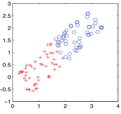
Figure 2: The two discriminative dimensions of our separable one hundred dimensional data set.
Here we report experiments on artificial data to illustrate how our algorithm works and how it compares to AdaBoost. Our data is 100 dimensional and contains 98 nuisance dimensions with uniform noise. The other two dimensions are plotted exemplary in Figure 2. For training we use only 100 examples which means that controlling the capacity of the ensemble is essential.
As the weak learning algorithm we use C4.5 decision trees provided by Quinlan (1992) using an option to control the number of nodes in the tree. We have tuned C4.5 to generate trees with about three nodes. Otherwise, the weak learner often classifies all training examples correctly and over-fits the data already. Furthermore, since in this case the margin is already maximum (equal to 1), boosting algorithms would stop sinceγ=1. We therefore need to limit the complexity of the weak learner, in good agreement with the bounds on the generalization error (Schapire et al., 1998). Moreover, we have to deal with the fact that C4.5 cannot use weighted samples. We therefore use weighted bootstrapping (e.g. Efron and Tibshirani, 1994). However, this amplifies the problem that the resulting hypotheses might in some cases have an edge smaller than the maximum margin, which according to the Min-Max-Theorem should not occur if the weak learner performs optimally. We deal with this problem by repeatedly calling C4.5 on different bootstrap realizations if the edge is smaller than the margin of the current linear combination. Furthermore, for AdaBoost∗ν, a small edge of one hypothesis can spoil the margin estimate ρt. We address this problem by resetting
ρt=ρˆt+ν, wheneverρt≤ρˆt, where ˆρt is the margin of the currently combined hypothesis.
In Figure 3 we see a typical run of AdaBoost, Marginal AdaBoost, AdaBoost∗νand Arc-GV for ν=.1. For comparison we plot the margins of the hypotheses generated by AdaBoost (cf. Figure 3 (left)). One observes that it is not able to achieve a large margin efficiently. After 1000 iterations
ˆ ρ=.37.
Marginal AdaBoost as proposed in R¨atsch and Warmuth (2002) proceeds in stages and first tries to find an estimate of the margin using a binary search. It calls AdaBoostρthree times. The first call of AdaBoostρforρ=0 stops after four iterations because it has generated a consistent combined hypothesis. The lower bound l onρ∗ as computed by Marginal AdaBoost is l=.07 and the upper bound u is.94. The second timeρis chosen to be in the middle of the interval[l,u]and AdaBoostρ reaches the margin ofρ=.51 after 80 iterations. The interval is now[.51, .77]. Because the length of the interval u−l=.27 is small enough, Marginal AdaBoost leaves the loop through an exit condition, calls AdaBoostρthe last time forρ=u−ν=.41 and finally achieves the margin of.55. In a run of Arc-GV for thousand iterations we observe a margin of the combined hypothesis of
.53, while for our new algorithm, AdaBoost∗ν, we find.58. In this case the margin for AdaBoost∗νis larger than the margins of all other algorithms when executed for one thousand iterations. It starts with slightly lower margins in the beginning, but then catches up due the better choice of the margin estimate.
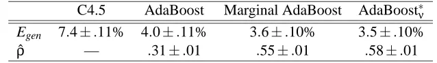
C4.5 AdaBoost Marginal AdaBoost AdaBoost∗ν Egen 7.4±.11% 4.0±.11% 3.6±.10% 3.5±.10%
ˆ
ρ — .31±.01 .55±.01 .58±.01
Figure 3: Illustration of the achieved margin of AdaBoost0 (left), Marginal AdaBoost (middle), Arc-GV, and AdaBoost∗ν (right) at each iteration. Marginal AdaBoost calls AdaBoostρ three times while adapting ρ (dash-dotted). We also plot the values for l and u as in Marginal AdaBoost (dashed). (For details see R¨atsch and Warmuth, 2002) AdaBoost∗ν achieves larger margins than AdaBoost. Compared to Arc-GV it starts slower, but then catches up in the later iterations. Here the correct choice of the parameterρis important.
In Table 2 we see the average performances of the four classifiers. For AdaBoost and AdaBoost∗ν we combined 200 hypotheses for the final prediction. For Marginal AdaBoost we useν=.1 and let the algorithm combine only 200 hypotheses for the final prediction to get a more fair comparison. We see a large improvement of all ensemble methods over the single classifier. There is also a slight, but – according to a t-test with confidence level 98% – significant difference between the generaliza-tion performances of AdaBoost and Marginal AdaBoost as well as AdaBoost and AdaBoost∗ν. Note also that the margins of the combined hypothesis achieved by Marginal AdaBoost and AdaBoost∗ν are on average almost twice as large as for AdaBoost. The difference in generalization performance between AdaBoost∗νand Marginal AdaBoost is not statistically significant.
The differences between the achieved margins of both algorithms seem slightly significant (96%). The slightly larger margins generated by Marginal AdaBoost can be attributed to the fact that it uses many more calls to the weak learner than AdaBoost∗νand after an estimate of the achievable margin is available, it starts optimizing the linear combination using this estimate.
It would be natural to use a two-pass algorithm: In the first pass use AdaBoost∗ν to get a margin estimateρsize at leastρ∗−νand then use this estimate in a final run of AdaBoostρ. The hypothesis produced in the second pass should have a larger margin and use fewer base hypotheses.
5.2 Heuristics for Tuning the Precision Parameterν
Our main results says that after 2 ln Nν2 iterations AdaBoost∗νproduces a hypothesis of margin at least
ρ∗−ν. Thus if the algorithm is allowed to run for T iterations, thenνshould be set toν
T=
q 2 ln N
T .
Ifνis chosen much larger thanνT, then after T iterations AdaBoost∗νoften achieves a margin below
ρ∗−ν
T. Similarly, ifνis chosen much smaller thanνT, then AdaBoost∗νstarts too slowly and after
T iterations its margin is typically again belowρ∗−νT.
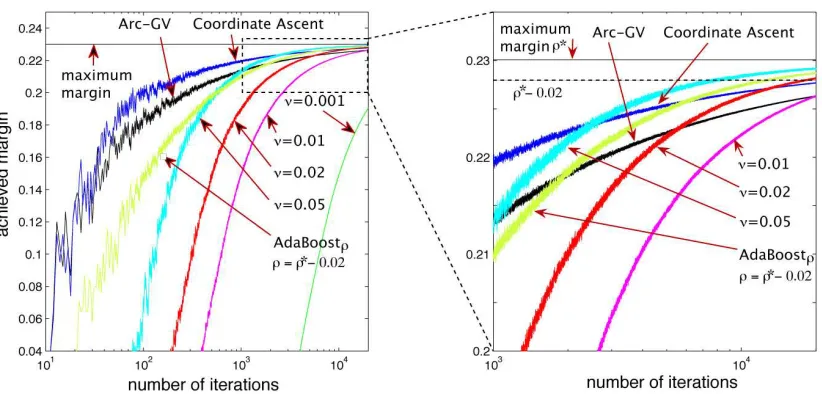
at most Ω(ν−3) iterations to achieve a margin of at leastρ∗−ν. While this theoretical result is clearly inferior to the guarantees which we provide for AdaBoost∗ν, their experimental evaluation of the algorithms seemed to suggest that the algorithm requires significantly fewer iterations than AdaBoost∗ν in practice. However, their observations were only due to the improper choice of the accuracy parameterνfor AdaBoost∗ν: For ν=10−3 (as chosen in their study), AdaBoost∗ν would need millions of iterations to achieve a guaranteed marginρ∗−ν. However, only the first 20K it-erations were displayed and in this range their algorithms achieve a larger margin. For T =20K and N=50, the precision parameter prescribed by our bounds isνT=.02. When this parameter is
used, then AdaBoost∗clearly beats all the other related algorithms (cf. Figure 4). We leave it to the reader to explore other heuristics for tuningνbased on the theoretical results of this paper (See also the discussion at the end of the last subsection).
Figure 4: AdaBoost∗νwith different choices ofνis compared to Arc-GV and the Coordinate Ascent Algorithm on the same artificial dataset 1 used in Rudin et al. (2004c) (We reconstructed this dataset from a figure given in Rudin et al. (2004b)): The number of iterations is T =20K, the dimension of the examples is N=50, and we assume that the base learner returns a hypothesis with maximum edge. Ifνis set to a reasonably close range around the valueνT=.02 prescribed by our bound, then AdaBoost∗νachieves the margin which is
significantly larger than the margins achieved by the other algorithms. Ifν=.001νT
6. Conclusion
We have analyzed a generalized version of AdaBoost in the context of large margin algorithms. From von Neumann’s Min-Max theorem we know that if the weak learner always returns a hypoth-esis with weighted classification error less than 12−1
2γthen the maximum achievable marginρ∗is at leastγ. The asymptotic analysis lead us to a lower bound on the margin of the final hypotheses generated by AdaBoostρ, which was shown to be rather tight in empirical cases. Our results indicate that vanilla AdaBoost generally does not maximize the margin, and only achieves a margin of about half the optimum.
To overcome these problems we provided an algorithm AdaBoost∗νwith the following provable guarantees: It produces a linear combination with margin at least ρ∗−νand the number of base hypotheses used in this linear combination is at most 2 ln nν2 . The new algorithm decreases its
esti-mateρ of the margin iteratively, such that the gap between the best and the worst case becomes arbitrarily small. Our analysis did not require additional properties of the weak learning algorithm. In simulation experiments we have illustrated the validity of our theoretical analysis.
Appendix A. Margins
First recall the definition of margin used in this paper, which is defined for a fixed set of exam-ples {(xn,yn): 1≤n≤N}and a set of hypotheses
H
={h1, . . . ,hM} (here finite for the sake ofsimplicity):
ρ∗(
H
) =maxα n=min1,...,Nyn M
∑
m=1
αmhm(xn),whereαis on the simplex
P
M.Note that we minimize over the margins of individual examples and maximize over the hyperplanes. Define the one-norm margin ρ∗1(
H
) in the same way but now α lies in the larger set {α:α∈RMand||α||1=1}.It is well known that for a fixed example(xn,yn)and normalα∈RM, the
one-norm margin∑Mm=1αmhm(xn)
∑M
m|αm| is the minimum`∞-distance of the example to the hyperplane with normal
α(Mangasarian, 1999; R¨atsch et al., 2002), where the latter distance is defined as
inf
z∈RMs.t.α·z=0 ynm=max1,...,M|hm(xn)−zm|.
Note that in this appendix, margins are defined as a function of the the hypotheses set
H
because we will vary this set in a moment. Let cl(H
) be the closure ofH
under negation, i.e. cl(H
) =H
∪ {−h : h∈H
}. Now, the following relationships are straightforward:1. ρ∗(
H
)≤ρ1∗(H
),ρ∗(cl(H
))≥0, andρ∗(cl(H
))≥ρ∗1(H
). 2. Ifρ∗(cl(H
))>0, thenρ∗(cl(H
)) =ρ∗1(H
).3. Ifρ∗1(
H
)≥0, thenρ∗(cl(H
)) =ρ∗ 1(H
).Appendix B. An Application to Multiple Kernel Learning
Sonnenburg et al. (2005) proposed a new algorithm for solving the multiple kernel learning (MKL) problem that was introduced in Lanckriet et al. (2004); Bach et al. (2004). The idea of MKL is to find a convex combination of J support vector kernels kj:
X
×X
7→R( j=1, . . . ,J) that maximizesthe SVM soft margin (cf. Bach et al. (2004)). In Sonnenburg et al. (2005) the original quadratically-constraint quadratic program was reformulated to the following semi-infinite linear program:
min β∈PJα∈supA
J
∑
j=1
βjSj(α) (9)
where
Sj(α) := −
1 2
N
∑
r,s=1
αrαsyryskj(xr,xs) + N
∑
n=1 αn
A
:=( α
α∈RN,0≤α≤1C,
N
∑
n=1
ynαn=0
)
and C is the SVM regularization constant. Note that this problem has infinitely many constraints: one for every vectorαin its domain
A
. Note that problem (9) is of the same type as the semi-infinite programming problem (8) which can be solved with AdaBoost∗ν (cf. discussion in Section 4.5). Since the Sj(α) are continuous functions andA
is compact, it follows from Theorem 8 that theduality gap is zero.
When AdaBoost∗ν is applied to this problem, a hypothesis with large edge has to be found in each iteration. In this case the hypotheses areαvectors and the edge is
J
∑
j=1
βjSj(α) =−
1
2
∑
r,sαrαsyrysJ
∑
j=1
βjkj(xr,xs)
!
+
∑
iαi.
It has been noted that the edge in this case is nothing else than the negative SVM objective function for the combined kernel k(xr,xs) =∑Jj=1βjkj(xr,xs). Hence, identifying anαvector with maximum
edge amounts to solving the vanilla SVM quadratic optimization problem. Fortunately, many effi-cient SVM packages are available to solve this problem. Thus, the MKL problem can be effieffi-ciently solved using AdaBoost∗νand our iteration bound for AdaBoost∗νis applicable.
References
F. R. Bach, G. R. G. Lanckriet, and M. I. Jordan. Multiple kernel learning, conic duality, and the SMO algorithm. In Twenty-first international conference on Machine learning. ACM Press, 2004. ISBN 1-58113-828-5.
K. P. Bennett, A. Demiriz, and J. Shawe-Taylor. A column generation algorithm for boosting. In P. Langley, editor, Proceedings, 17th ICML, pages 65–72, San Francisco, 2000. Morgan Kauf-mann.
L. Breiman. Prediction games and arcing algorithms. Neural Computation, 11(7):1493–1518, 1999. Also Technical Report 504, Statistics Department, University of California Berkeley, Dec. 1997. B. Efron and R. J. Tibshirani. An Introduction to the Bootstrap, volume 57 of Monographs on
Statistic and Applied Probability. Chapman and Hall/CRC, New York, 1994.
Y. Freund. Boosting a weak learning algorithm by majority. Information and Computation, 121(2): 256–285, September 1995.
Y. Freund and R. E. Schapire. Experiments with a new boosting algorithm. In Proc. 13th Interna-tional Conference on Machine Learning, pages 148–146. Morgan Kaufmann, 1996.
Y. Freund and R. E. Schapire. A decision-theoretic generalization of on-line learning and an appli-cation to boosting. Journal of Computer and System Sciences, 55(1):119–139, 1997.
Y. Freund and R. E. Schapire. Adaptive game playing using multiplicative weights. Games and Economic Behavior, 29:79–103, 1999.
A. J. Grove and D. Schuurmans. Boosting in the limit: Maximizing the margin of learned ensembles. In Proceedings of the Fifteenth National Conference on Artifical Intelligence, 1998.
R. Hettich and K. O. Kortanek. Semi-infinite programming: Theory, methods and applications. SIAM Review, 3:380–429, September 1993.
J. Kivinen and M. Warmuth. Boosting as entropy projection. In Proc. 12th Annu. Conference on Comput. Learning Theory, pages 134–144. ACM Press, New York, NY, 1999.
V. Koltchinskii, D. Panchenko, and F. Lozano. Some new bounds on the generalization error of combined classifiers. In Advances in Neural Information Processing Systems, volume 13, 2001. J. Lafferty. Additive models, boosting, and inference for generalized divergences. In Proc. 12th
Annu. Conf. on Comput. Learning Theory, pages 125–133, New York, NY, 1999. ACM Press.
G. R. G. Lanckriet, T. De Bie, N. Cristianini, M. I. Jordan, and W. S. Noble. A statistical framework for genomic data fusion. Bioinformatics, 2004.
O. L. Mangasarian. Arbitrary-norm separating plane. Operation Research Letters, 24(1):15–23, 1999.
S. Nash and A. Sofer. Linear and Nonlinear Programming. McGraw-Hill, New York, NY, 1996. J. R. Quinlan. C4.5: Programs for Machine Learning. Morgan Kaufmann, 1992.
J. R. Quinlan. Boosting first-order learning. Lecture Notes in Computer Science, 1160:143, 1996. G. R¨atsch. Robust Boosting via Convex Optimization. PhD thesis, University of Potsdam, Neues
Palais 10, 14469 Potsdam, Germany, October 2001.
G. R¨atsch, S. Mika, B. Sch¨olkopf, and K.-R. M¨uller. Constructing boosting algorithms from SVMs: an application to one-class classification. IEEE PAMI, 24(9), September 2002. In press. Earlier version is GMD TechReport No. 119, 2000.
G. R¨atsch, T. Onoda, and K.-R. M¨uller. Soft margins for AdaBoost. Machine Learning, 42(3): 287–320, March 2001. Also NeuroCOLT Technical Report NC-TR-1998-021.
G. R¨atsch and M. K. Warmuth. Maximizing the margin with boosting. In Proc. COLT, volume 2375 of LNAI, pages 319–333, Sydney, 2002. Springer.
S. Rosset, J. Zhu, and T. Hastie. Boosting as a regularized path to a maximum margin separator. Technical report, Department of Statistics, Stanford University, 2002.
C. Rudin, I. Daubechies, and R. E. Schapire. On the dynamics of boosting. In Advances in Neural Information Processing, volume 15, 2004a.
C. Rudin, I. Daubechies, and R. E. Schapire. The dynamics of AdaBoost: Cyclic behavior and convergence of margins. Journal of Machine Learning Research, 2005.
C. Rudin, R. E. Schapire, and I. Daubechies. Analysis of boosting algoritms using the smooth margin function: A study of three algorithms. Unpublished manuscript, October 2004b.
C. Rudin, R. E. Schapire, and I. Daubechies. Boosting based on a smooth margin. In Proc. COLT’04, LNCS. Springer Verlag, July 2004c.
R. E. Schapire. The Design and Analysis of Efficient Learning Algorithms. PhD thesis, MIT Press, 1992.
R. E. Schapire, Y. Freund, P. L. Bartlett, and W. S. Lee. Boosting the margin: A new explanation for the effectiveness of voting methods. The Annals of Statistics, 26(5):1651–1686, October 1998. R. E. Schapire and Y. Singer. Improved boosting algorithms using confidence-rated predictions.
Machine Learning, 37(3):297–336, December 1999.
S. Sonnenburg, G. R¨atsch, and C. Sch¨afer. Learning interpretable svms for biological sequence analysis. In Proc. RECOMB’05, LNCB. Springer Verlag, 2005.
J. von Neumann. Zur Theorie der Gesellschaftsspiele. Math. Ann., 100:295–320, 1928.
![Figure 1: Achieved margins of AdaBoostρ using the best (green) and the worst (red) selection on randomdata for ρ = 0 [left] and ρ = 13 [right]](https://thumb-us.123doks.com/thumbv2/123dok_us/9841075.1970470/12.612.95.514.82.286/figure-achieved-margins-adaboostr-using-green-selection-randomdata.webp)