Working Set Selection Using Second Order Information
for Training Support Vector Machines
Rong-En Fan [email protected]
Pai-Hsuen Chen [email protected]
Chih-Jen Lin [email protected]
Department of Computer Science, National Taiwan University Taipei 106, Taiwan
Editor:Thorsten Joachims
Abstract
Working set selection is an important step in decomposition methods for training support vector machines (SVMs). This paper develops a new technique for working set selection in SMO-type decomposition methods. It uses second order information to achieve fast con-vergence. Theoretical properties such as linear convergence are established. Experiments demonstrate that the proposed method is faster than existing selection methods using first order information.
Keywords: support vector machines, decomposition methods, sequential minimal opti-mization, working set selection
1. Introduction
Support vector machines (SVMs) (Boser et al., 1992; Cortes and Vapnik, 1995) are a useful classification method. Given instances xi, i = 1, . . . , l with labels yi ∈ {1,−1}, the main task in training SVMs is to solve the following quadratic optimization problem:
min α
f(α) = 1 2α
TQα−eTα
subject to 0≤αi≤C, i= 1, . . . , l, (1)
yTα= 0,
where e is the vector of all ones, C is the upper bound of all variables, Q is an l by l symmetric matrix withQij =yiyjK(xi,xj), andK(xi,xj) is the kernel function.
Algorithm 1 (SMO-type decomposition method)
1. Find α1 as the initial feasible solution. Set k= 1.
2. If αk is an optimal solution of (1), stop. Otherwise, find a two-element working set B = {i, j} ⊂ {1, . . . , l}. Define N ≡ {1, . . . , l}\B and αkB and αkN to be sub-vectors of αk corresponding toB and N, respectively.
3. Solve the following sub-problem with the variable αB:
min α B 1 2
αTB (αkN)T
QBB QBN QN B QN N
αB
αkN
−
eT
B eTN
αB
αkN
= 1 2α
T
BQBBαB+ (−eB+QBNαkN)TαB+ constant
= 1 2
αi αj
Qii Qij Qij Qjj
αi αj
+ (−eB+QBNαkN)T
αi αj
+ constant
subject to 0≤αi, αj ≤C, (2)
yiαi+yjαj =−yTNαkN,
wherehQBB QBN
QN BQN N i
is a permutation of the matrix Q.
4. SetαkB+1 to be the optimal solution of (2) and αNk+1 ≡αkN. Set k←k+ 1 and goto Step 2.
Note that the setB changes from one iteration to another, but to simplify the notation, we just use B instead ofBk.
Since only few components are updated per iteration, for difficult problems, the decom-position method suffers from slow convergences. Better methods of working set selection could reduce the number of iterations and hence are an important research issue. Existing methods mainly rely on the violation of the optimality condition, which also corresponds to first order (i.e., gradient) information of the objective function. Past optimization research indicates that using second order information generally leads to faster convergence. Now (1) is a quadratic programming problem, so second order information directly relates to the decrease of the objective function. There are several attempts (e.g., Lai et al., 2003a,b) to find working sets based on the reduction of the objective value, but these selection methods are only heuristics without convergence proofs. Moreover, as such techniques cost more than existing ones, fewer iterations may not lead to shorter training time. This paper de-velops a simple working set selection using second order information. It can be extended for indefinite kernel matrices. Experiments demonstrate that the training time is shorter than existing implementations.
2. Existing and New Working Set Selections
In this section, we discuss existing methods of working set selection and then propose a new approach.
2.1 Existing Selections
Currently a popular way to select the working setB is via the “maximal violating pair:”
WSS 1 (Working set selection via the “maximal violating pair”)
1. Select
i∈arg max
t {−yt∇f(α
k)t|t∈I
up(αk)},
j∈arg min
t {−yt∇f(α
k)t|t∈I
low(αk)}, where
Iup(α)≡ {t|αt< C, yt= 1 orαt>0, yt=−1}, and Ilow(α)≡ {t|αt< C, yt=−1 or αt>0, yt= 1}.
(3)
2. Return B={i, j}.
This working set was first proposed in Keerthi et al. (2001) and is used in, for example, the software LIBSVM (Chang and Lin, 2001). WSS 1 can be derived through the Karush-Kuhn-Tucker (KKT) optimality condition of (1): A vector α is a stationary point of (1) if and only if there is a numberb and two nonnegative vectorsλand µsuch that
∇f(α) +by=λ−µ,
λiαi= 0, µi(C−αi) = 0, λi ≥0, µi ≥0, i= 1, . . . , l,
where∇f(α)≡Qα−eis the gradient of f(α). This condition can be rewritten as
∇f(α)i+byi ≥0 ifαi < C, (4)
∇f(α)i+byi ≤0 ifαi >0. (5)
Since yi=±1, by defining Iup(α) and Ilow(α) as in (3), and rewriting (4)-(5) to −yi∇f(α)i ≤b,∀i∈Iup(α), and
−yi∇f(α)i ≥b,∀i∈Ilow(α), a feasibleα is a stationary point of (1) if and only if
m(α)≤M(α), (6)
where
m(α)≡ max i∈Iup(α)
−yi∇f(α)i, and M(α)≡ min i∈Ilow(α)
−yi∇f(α)i.
Note that m(α) and M(α) are well defined except a rare situation where all yi = 1 (or −1). In this case the zero vector is the only feasible solution of (1), so the decomposition method stops at the first iteration.
Definition 1 (Violating pair) If i∈Iup(α), j ∈Ilow(α), and −yi∇f(α)i>−yj∇f(α)j,
then{i, j} is a “violating pair.”
From (6), indices{i, j} which most violate the optimality condition are a natural choice of the working set. They are called a “maximal violating pair” in WSS 1. It is known that violating pairs are important in the working set selection:
Theorem 2 (Hush and Scovel, 2003) Assume Q is positive semi-definite. SMO-type
methods have the strict decrease of the function value (i.e., f(αk+1) < f(αk),∀k) if and
only ifB is a violating pair.
Interestingly, the maximal violating pair is related to first order approximation of f(α). As explained below,{i, j} selected via WSS 1 satisfies
{i, j}= arg min
B:|B|=2Sub(B), (7)
where
Sub(B)≡min
dB ∇f(α
k)T
BdB (8a)
subject to yBTdB= 0,
dt≥0, ifαkt = 0, t∈B, (8b)
dt≤0, ifαkt =C, t∈B, (8c)
−1≤dt≤1, t∈B. (8d)
Problem (7) was first considered in Joachims (1998). By defining dT ≡ [dT
B,0TN], the objective function (8a) comes from minimizing first order approximationof f(αk+d):
f(αk+d) ≈ f(αk) +∇f(αk)Td
= f(αk) +∇f(αk)T BdB.
The constraintyT
BdB= 0 is fromyT(αk+d) = 0 andyTαk= 0. The condition 0≤αt≤C leads to inequalities (8b) and (8c). As (8a) is a linear function, the inequalities −1≤dt≤ 1, t∈B avoid that the objective value goes to −∞.
A first look at (7) indicates that we may have to check all 2l
B’s in order to find an optimal set. Instead, WSS 1 efficiently solves (7) in O(l) steps. This result is discussed in Lin (2001b, Section II), where more general settings (|B|is any even integer) are considered. The proof for|B|= 2 is easy, so we give it in Appendix A for completeness.
The convergence of the decomposition method using WSS 1 is proved in Lin (2001b, 2002).
2.2 A New Working Set Selection
Instead of using first order approximation, we may consider more accurate second order information. Asf is a quadratic,
f(αk+d)−f(αk) = ∇f(αk)Td+1 2d
T∇2f(αk)d = ∇f(αk)TBdB+
1 2d
T
is exactly the reduction of the objective value. Thus, by replacing the objective function of (8) with (9), a selection method usingsecond order information is
min
B:|B|=2Sub(B), (10)
where
Sub(B)≡min
d
B
1 2d
T
B∇2f(αk)BBdB+∇f(αk)TBdB (11a)
subject to yBTdB= 0, (11b)
dt≥0, ifαkt = 0, t∈B, (11c) dt≤0, ifαkt =C, t∈B. (11d)
Note that inequality constraints −1 ≤ dt ≤ 1, t ∈ B in (8) are removed, as later we will see that the optimal value of (11) does not go to −∞. Though one expects (11) is better than (8), minB:|B|=2Sub(B) in (10) becomes a challenging task. Unlike (7)-(8), which can be efficiently solved by WSS 1, for (10) and (11) there is no available way to avoid checking all 2l
B’s. Note that except the working set selection, the main task per decomposition iteration is on calculating the two kernel columns Qti and Qtj, t = 1, . . . , l. This requires O(l) operations and is needed only ifQis not stored. Therefore, each iteration can become l times more expensive if an O(l2) working set selection is used. Moreover, from simple experiments we know that the number of iterations is, however, not decreased l times. Therefore, anO(l2) working set selection is impractical.
A viable implementation of using second order information is thus to heuristically check several B’s only. We propose the following new selection:
WSS 2 (Working set selection using second order information)
1. Select
i∈arg max
t {−yt∇f(α
k)t|t∈I
up(αk)}. 2. Consider Sub(B) defined in (11) and select
j∈arg min
t {Sub({i, t})|t∈Ilow(α k),−y
t∇f(αk)t<−yi∇f(αk)i}. (12)
3. Return B={i, j}.
By using the sameias in WSS 1, we check onlyO(l) possibleB’s to decidej. Alternatively, one may choose j ∈argM(αk) and search for iby a way similar to (12)1. In fact, such a selection is the same as swapping labelsyfirst and then applying WSS 2, so the performance should not differ much. It is certainly possible to consider other heuristics, and the main concern is how good they are if compared to the one by fully checking all 2l
sets. In Section 7 we will address this issue. Experiments indicate that a full check does not reduce iterations of using WSS 2 much. Thus WSS 2 is already a very good way of using second order information.
1. To simplify the notations, we denote argM(α) as arg mint∈Ilow(α)−yt∇f(α)t and argm(α) as
Despite the above issue of how to effectively use second order information, the real challenge is whether the new WSS 2 can cause shorter training time than WSS 1. Now the two selection methods differ only in selecting j, so we can also consider WSS 2 as a direct attempt to improve WSS 1. The following theorem shows that one could efficiently solve (11), so the working set selection WSS 2 does not cost a lot more than WSS 1.
Theorem 3 If B ={i, j} is a violating pair and Kii+Kjj −2Kij >0, then (11) has the
optimal objective value
−(−yi∇f(α k)i+y
j∇f(αk)j)2 2(Kii+Kjj−2Kij)
.
Proof Define ˆdi≡yidi and ˆdj ≡yjdj. From yTBdB = 0, we have ˆdi =−dˆj and
1 2
di dj
Qii Qij Qij Qjj
di dj
+
∇f(αk)i ∇f(αk)j
di dj
= 1
2(Kii+Kjj−2Kij) ˆd 2
j + (−yi∇f(αk)i+yj∇f(αk)j) ˆdj. (13)
Since Kii+Kjj−2Kij >0 and B is a violating pair, we can define
aij ≡Kii+Kjj−2Kij >0 and bij ≡ −yi∇f(αk)i+yj∇f(αk)j >0. (14)
Then (13) has the minimum at
ˆ
dj =−dˆi =− bij aij
<0, (15)
and
the objective function (11a) =− b 2 ij 2aij
.
Moreover, we can show that ˆdi and ˆdj (di and dj) indeed satisfy (11c)-(11d). If j ∈ Ilow(αk), αkj = 0 implies yj = −1 and hence dj = yjdˆj > 0, a condition required by (11c). Other cases are similar. Thus ˆdi and ˆdi defined in (15) are optimal for (11).
Note that if K is positive definite, then for any i 6= j, Kii+Kjj −2Kij > 0. Using Theorem 3, (12) in WSS 2 is reduced to a very simple form:
j∈arg min t
−b
2 it ait
|t∈Ilow(αk),−yt∇f(αk)t<−yi∇f(αk)i
,
whereaitand bitare defined in (14). If K is not positive definite, the leading coefficientaij of (13) may be non-positive. This situation will be addressed in the next sub-section.
Note that (8) and (11) are used only for selecting the working set, so they do not have to maintain the feasibility 0 ≤ αk
selection procedure is more complicated than solving the sub-problem (11). Besides, these earlier approaches do not provide any convergence analysis. In Section 6 we will investigate the issue of maintaining feasibility in the selection procedure, and explain why using (11) is better.
2.3 Non-Positive Definite Kernel Matrices
Theorem 3 does not hold if Kii+Kjj −2Kij ≤ 0. For the linear kernel, sometimes K is only positive semi-definite, so it is possible that Kii+Kjj −2Kij = 0. Moreover, some existing kernel functions (e.g., sigmoid kernel) are not the inner product of two vectors, so K is even not positive semi-definite. Then Kii+Kjj−2Kij <0 may occur and (13) is a concave objective function.
Once B is decided, the same difficulty occurs for the sub-problem (2) to obtain αk+1. Note that (2) differs from (11) only in constraints; (2) strictly requires the feasibility 0≤αi+ di≤C,∀t∈B. Therefore, (2) also has a concave objective function ifKii+Kjj−2Kij <0. In this situation, (2) may possess multiple local minima. Moreover, there are difficulties in proving the convergence of the decomposition methods (Palagi and Sciandrone, 2005; Chen et al., 2006). Thus, Chen et al. (2006) proposed adding an additional term to (2)’s objective function if aij ≡Kii+Kjj−2Kij ≤0:
min αi,αj
1 2
αi αj
Qii Qij Qij Qjj
αi αj
+ (−eB+QBNαkN)T
αi αj
+
τ −aij
4 ((αi−α k
i)2+ (αj −αkj)2)
subject to 0≤αi, αj ≤C, (16)
yiαi+yjαj =−yTNαkN,
where τ is a small positive number. By defining ˆdi ≡ yi(αi−αik) and ˆdj ≡ yj(αj −αkj), (16)’s objective function, in a form similar to (13), is
1 2τdˆ
2
j +bijdˆj, (17)
wherebij is defined as in (14). The new objective function is thus strictly convex. If{i, j} is a violating pair, then a careful check shows that there is ˆdj <0 which leads to a negative value in (17) and maintains the feasibility of (16). Therefore, we can find αk+1 6= αk
satisfying f(αk+1)< f(αk). More details are in Chen et al. (2006).
For selecting the working set, we consider a similar modification: If B ={i, j} and aij is defined as in (14), then (11) is modified to:
Sub(B)≡min dB
1 2d
T
B∇2f(αk)BBdB+∇f(αk)TBdB+
τ−aij 4 (d
2 i +d2j) subject to constraints of (11).
(18)
Note that (18) differs from (16) only in constraints. In (18) we do not maintain the feasibility of αk
By reformulating (18) to (17) and following the same argument in Theorem 3, the optimal objective value of (18) is
−b 2 ij 2τ.
Therefore, a generalized working set selection is as the following:
WSS 3
(Working set selection using second order information: any symmetric K)
1. Define ats and bts as in (14), and
¯ ats≡
ats ifats >0,
τ otherwise. (19)
Select
i ∈ arg max
t {−yt∇f(α k)
t|t∈Iup(αk)},
j ∈ arg min t
−b
2 it ¯ ait
|t∈Ilow(αk),−yt∇f(αk)t<−yi∇f(αk)i
. (20)
2. Return B={i, j}.
In summary, an SMO-type decomposition method using WSS 3 for the working set selection is:
Algorithm 2 (An SMO-type decomposition method using WSS 3)
1. Find α1 as the initial feasible solution. Set k= 1.
2. If αk is a stationary point of (1), stop. Otherwise, find a working set B ={i, j} by WSS 3.
3. Let aij be defined as in (14). Ifaij >0, solve the sub-problem (2). Otherwise, solve (16). SetαkB+1 to be the optimal point of the sub-problem.
4. SetαkN+1 ≡αkN. Setk←k+ 1 and goto Step 2.
In the next section we study theoretical properties of using WSS 3.
3. Theoretical Properties
To obtain theoretical properties of using WSS 3, we consider the work (Chen et al., 2006), which gives a general study of SMO-type decomposition methods. It considers Algorithm 2 but replaces WSS 3 with a general working set selection2:
WSS 4 (A general working set selection discussed in Chen et al., 2006)
1. Consider a fixed 0< σ≤1 for all iterations.
2. Select anyi∈Iup(αk), j∈Ilow(αk) satisfying
−yi∇f(αk)i+yj∇f(αk)j ≥σ(m(αk)−M(αk))>0. (21)
3. Return B={i, j}.
Clearly (21) ensures the quality of the selected pair by linking it to the maximal violating pair. It is easy to see that WSS 3 is a special case of WSS 4: AssumeB ={i, j} is the set returned from WSS 3 and ¯j∈argM(αk). Since WSS 3 selectsi∈argm(αk), with ¯aij >0 and ¯ai¯j >0, (20) in WSS 3 implies
−(−yi∇f(αk)i+yj∇f(αk)j)2 ¯
aij
≤ −(m(α
k)−M(αk))2 ¯
ai¯j
.
Thus,
−yi∇f(αk)i+yj∇f(αk)j ≥ s
mint,s¯at,s maxt,s¯at,s
(m(αk)−M(αk)),
an inequality satisfying (21) forσ =p
mint,s¯at,s/maxt,sa¯t,s.
Therefore, all theoretical properties proved in Chen et al. (2006) hold here. They are listed below.
It is known that the decomposition method may not converge to an optimal solution if using improper methods of working set selection. We thus must prove that the proposed selection leads to the convergence.
Theorem 4 (Asymptotic convergence (Chen et al., 2006, Theorem 3 and Corol-lary 1))
Let {αk} be the infinite sequence generated by the SMO-type method Algorithm 2. Then
any limit point of {αk} is a stationary point of (1). Moreover, if Q is positive definite,
{αk} globally converges to the unique minimum of (1).
As the decomposition method only asymptotically approaches an optimum, in practice, it is terminated after satisfying a stopping condition. For example, we can pre-specify a small tolerance >0 and check if the maximal violation is small enough:
m(αk)−M(αk)≤. (22)
Alternatively, one may check if the selected working set{i, j} satisfies
−yi∇f(αk)i+yj∇f(αk)j ≤, (23)
Theorem 5 (Finite termination and explanation of caching and shrinking tech-niques (Chen et al., 2006, Theorems 4 and 6))
Assume Q is positive semi-definite.
1. The following set is independent of any optimal solution α¯:
I ≡ {i| −yi∇f( ¯α)i> M( ¯α) or −yi∇f( ¯α)i < m( ¯α)}. (24)
Problem (1) has unique and bounded optimal solutions at αi, i∈I.
2. Assume Algorithm 2 generates an infinite sequence {αk}. There isk¯ such that after
k≥¯k, everyαk
i, i∈I has reached the unique and bounded optimal solution. It remains
the same in all subsequent iterations and ∀k≥¯k:
i6∈ {t|M(αk)≤ −yt∇f(αk)t≤m(αk)}. (25)
3. If (1) has an optimal solution α¯ satisfying m( ¯α) < M( ¯α), then α¯ is the unique
solution and Algorithm 2 reaches it in a finite number of iterations.
4. If {αk} is an infinite sequence, then the following two limits exist and are equal:
lim k→∞m(α
k) = lim k→∞M(α
k) =m( ¯α) =M( ¯α), (26)
where α¯ is any optimal solution.
Finally, the following theorem shows that Algorithm 2 is linearly convergent under some assumptions:
Theorem 6 (Linear convergence (Chen et al., 2006, Theorem 8))
Assume problem (1) satisfies
1. Q is positive definite. Therefore, (1) has a unique optimal solution α¯.
2. The nondegenency condition. That is, the optimal solution α¯ satisfies that
∇f( ¯α)i+ ¯byi= 0 if and only if 0<α¯i < C, (27)
where ¯b=m( ¯α) =M( ¯α) according to Theorem 5.
For the sequence {αk} generated by Algorithm 2, there are c < 1 and ¯k such that for all
k≥¯k,
f(αk+1)−f( ¯α)≤c(f(αk)−f( ¯α)).
This theorem indicates how fast the SMO-type method Algorithm 2 converges. For any fixed problem (1) and a given tolerance , there is ¯ksuch that within
¯
k+O(1/)
iterations,
|f(αk)−f( ¯α)| ≤.
Note thatO(1/) iterations are necessary for decomposition methods according to the anal-ysis in Lin (2001a)3. Hence the result of linear convergence here is already the best worst case analysis.
4. Extensions
The proposed WSS 3 can be directly used for training support vector regression (SVR) and one-class SVM because they solve problems similar to (1). More detailed discussion about applying WSS 4 (and hence WSS 3) to SVR and one-class SVM is in Chen et al. (2006, Section IV).
Another formula which needs special attention is ν-SVM (Sch¨olkopf et al., 2000), which solves a problem with one more linear constraint:
min
α f(α) = 1 2α
TQα
subject to yTα= 0, (28)
eTα=ν,
0≤αi ≤1/l, i= 1, . . . , l,
whereeis the vector of all ones and 0≤ν≤1.
Similar to (6), α is a stationary point of (28) if and only if it satisfies
mp(α)≤Mp(α) and mn(α)≤Mn(α), (29)
where
mp(α)≡ max i∈Iup(α),yi=1
−yi∇f(α)i, Mp(α)≡ min i∈Ilow(α),yi=1
−yi∇f(α)i, and
mn(α)≡ max i∈Iup(α),yi=−1
−yi∇f(α)i, Mn(α)≡ min i∈Ilow(α),yi=−1
−yi∇f(α)i.
A detailed derivation is in, for example, Chen et al. (2006, Section VI).
In an SMO-type method for ν-SVM the selected working set B = {i, j} must satisfy yi = yj. Otherwise, if yi 6= yj, then the two linear equalities make the sub-problem have only one feasible pointαkB. Therefore, to select the working set, one considers positive (i.e., yi = 1) and negative (i.e.,yi =−1) instances separately. Existing implementations such as
LIBSVM (Chang and Lin, 2001) check violating pairs in each part and select the one with
the largest violation. This strategy is an extension of WSS 1. By a derivation similar to that in Section 2, the selection can also be from first or second order approximation of the objective function. Using Sub({i, j}) defined in (11), WSS 2 in Section 2 is modified to
WSS 5 (Extending WSS 2 for ν-SVM)
1. Find
ip∈argmp(αk),
jp∈arg min
t {Sub({ip, t})|yt= 1,αt∈Ilow(α k),−y
t∇f(αk)t<−yip∇f(α
k)i
p}.
2. Find
in∈argmn(αk),
jn∈arg min
t {Sub({in, t})|yt=−1,αt∈Ilow(α k),−y
t∇f(αk)t<−yin∇f(α
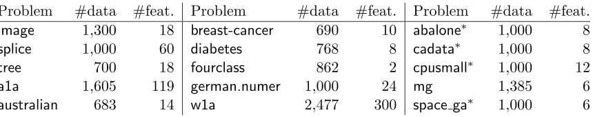
Problem #data #feat. Problem #data #feat. Problem #data #feat.
image 1,300 18 breast-cancer 690 10 abalone∗ 1,000 8
splice 1,000 60 diabetes 768 8 cadata∗ 1,000 8
tree 700 18 fourclass 862 2 cpusmall∗ 1,000 12
a1a 1,605 119 german.numer 1,000 24 mg 1,385 6
australian 683 14 w1a 2,477 300 space ga∗ 1,000 6
Table 1: Data statistics for small problems (left two columns: classification, right column: regression). ∗: subset of the original problem.
3. Check Sub({ip, jp}) and Sub({in, jn}). Return the set with a smaller value.
By Theorem 3 in Section 2, it is easy to solve Sub({ip, t}) and Sub({in, t}) in the above procedure.
5. Experiments
In this section we aim at comparing the proposed WSS 3 with WSS 1, which selects the maximal violating pair. As indicated in Section 2, they differ only in finding the second element j: WSS 1 checks first order approximation of the objective function, but WSS 3 uses second order information.
5.1 Data and Experimental Settings
First, some small data sets (around 1,000 samples) including ten binary classification and five regression problems are investigated under various settings. Secondly, observations are further confirmed by using four large (more than 30,000 instances) classification problems. Data statistics are in Tables 1 and 3.
Problems german.numer and australian are from the Statlog collection (Michie et al., 1994). We selectspace gaandcadatafrom StatLib (http://lib.stat.cmu.edu/datasets). The data sets image, diabetes, covtype, breast-cancer, and abalone are from the UCI ma-chine learning repository (Blake and Merz, 1998). Problems a1a and a9a are compiled in Platt (1998) from the UCI “adult” data set. Problems w1a and w8a are also from Platt (1998). The tree data set was originally used in Bailey et al. (1993). The problem mg is a Mackey-Glass time series. The data sets cpusmall and splice are from the Delve archive
(http://www.cs.toronto.edu/~delve). Problemfourclassis from Ho and Kleinberg (1996)
and we further transform it to a two-class set. The problemIJCNN1is from the first problem of IJCNN 2001 challenge (Prokhorov, 2001).
For most data sets each attribute is linearly scaled to [−1,1]. We do not scale a1a,a9a,
w1a, andw8aas they take two values 0 and 1. Another exception iscovtype, in which 44 of 54 features have 0/1 values. We scale only the other ten features to [0,1]. All data are available
athttp://www.csie.ntu.edu.tw/~cjlin/libsvmtools/. We use LIBSVM(version 2.71)
Different SVM parameters such as C in (1) and kernel parameters affect the training time. It is difficult to evaluate the two methods under every parameter setting. To have a fair comparison, we simulate how one uses SVM in practice and consider the following procedure:
1. “Parameter selection” step: Conduct five-fold cross validation to find the best one within a given set of parameters.
2. “Final training” step: Train the whole set with the best parameter to obtain the final model.
For each step we check time and iterations using the two methods of working set selection. For some extreme parameters (e.g., very large or small values) in the “parameter selection” step, the decomposition method converges very slowly, so the comparison shows if the proposed WSS 3 saves time under difficult situations. On the other hand, the best parameter usually locates in a more normal region, so the “final training” step tests if WSS 3 is competitive with WSS 1 for easier cases.
The behavior of using different kernels is a concern, so we thoroughly test four commonly used kernels:
1. RBF kernel:
K(xi,xj) =e−γk
xi−xjk2
.
2. Linear kernel:
K(xi,xj) =xTi xj.
3. Polynomial kernel:
K(xi,xj) = (γ(xTi xj+ 1))d.
4. Sigmoid kernel:
K(xi,xj) = tanh(γxTi xj+d).
Note that this function cannot be represented asφ(xi)Tφ(xj) under some parameters. Then the matrixQis not positive semi-definite. Experimenting with this kernel tests if our extension to indefinite kernels in Section 2.3 works well or not.
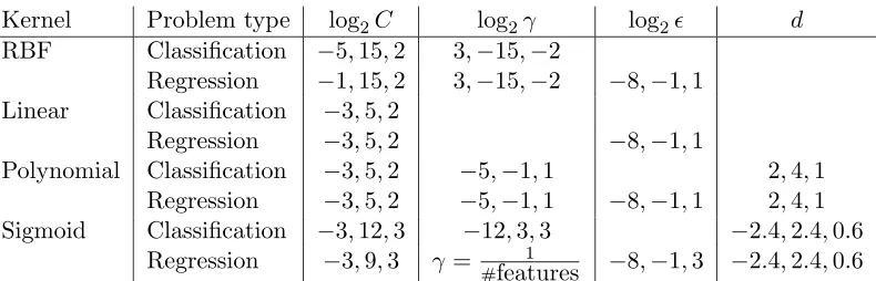
Parameters used for each kernel are listed in Table 2. Note that as SVR has an additional parameter, to save the running time, for other parameters we may not consider as many values as in classification.
It is important to check how WSS 3 performs after incorporating shrinking and caching strategies. Such techniques may effectively save kernel evaluations at each iteration, so the higher cost of WSS 3 is a concern. We consider various settings:
1. With or without shrinking.
Kernel Problem type log2C log2γ log2 d RBF Classification −5,15,2 3,−15,−2
Regression −1,15,2 3,−15,−2 −8,−1,1 Linear Classification −3,5,2
Regression −3,5,2 −8,−1,1
Polynomial Classification −3,5,2 −5,−1,1 2,4,1 Regression −3,5,2 −5,−1,1 −8,−1,1 2,4,1 Sigmoid Classification −3,12,3 −12,3,3 −2.4,2.4,0.6
Regression −3,9,3 γ = 1
#features −8,−1,3 −2.4,2.4,0.6 Table 2: Parameters used for various kernels: values of each parameter are from a uniform
discretization of an interval. We list the left, right end points and the space for discretization. For example,−5,15,2 for log2C means log2C =−5,−3, . . . ,15.
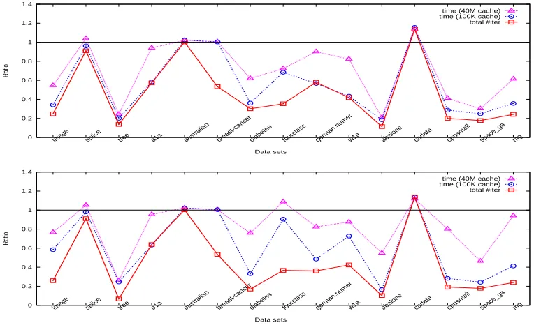
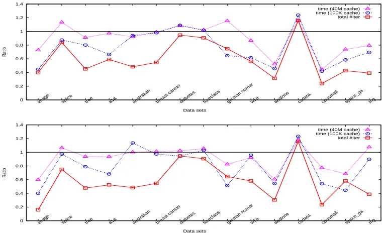
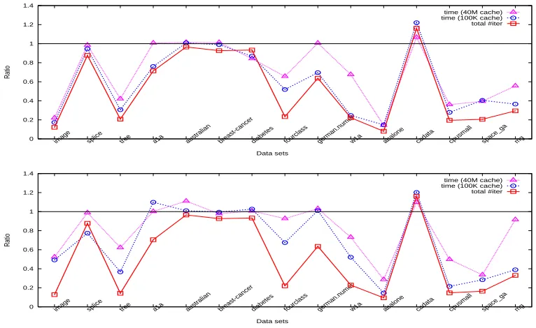
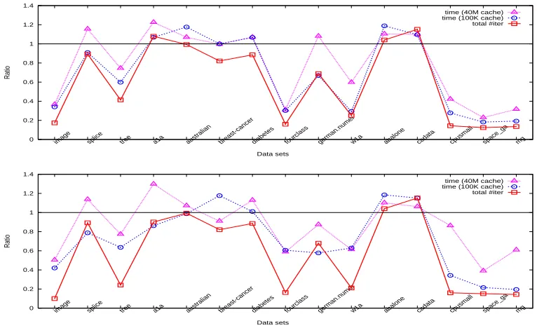
For each kernel, we give two figures showing results of “parameter selection” and “final training” steps, respectively. We further separate each figure to two scenarios: without/with shrinking, and present three ratios between using WSS 3 and using WSS 1:
ratio 1 ≡ # iter. by Alg. 2 with WSS 3 # iter. by Alg. 2 with WSS 1,
ratio 2 ≡ time by Alg. 2 (WSS 3, 100K cache) time by Alg. 2 (WSS 1, 100K cache),
ratio 3 ≡ time by Alg. 2 (WSS 3, 40M cache) time by Alg. 2 (WSS 1, 40M cache).
Note that the number of iterations is independent of the cache size. For the “parameter selection” step, time (or iterations) of all parameters is summed up before calculating the ratio. In general the “final training” step is very fast, so the timing result may not be accurate. Hence we repeat this step several times to obtain more reliable timing values. Figures 1-8 present obtained ratios. They are in general smaller than one, so using WSS 3 is really better than using WSS 1. Before describing other results, we explain an interesting observation: In these figures, if shrinking is not used, in general
ratio 1≤ratio 2≤ratio 3. (30)
Under the two very different cache sizes, one is too small to store the kernel matrix, but the other is large enough. Thus, roughly we have
time per Alg. 2 iteration (100K cache) ≈ Calculating twoQcolumns + Selection, time per Alg. 2 iteration (40M cache) ≈ Selection.
(31)
If shrinking is not used, the optimization problem is not reduced and hence
time by Alg. 2
0 0.2 0.4 0.6 0.8 1 1.2 1.4
image splice tree a1a australian breast-cancerdiabetes fourclass german.numerw1a abalone cadata cpusmall space_ga mg
Ratio
Data sets
time (40M cache) time (100K cache) total #iter
0 0.2 0.4 0.6 0.8 1 1.2 1.4
image splice tree a1a australian breast-cancerdiabetes fourclass german.numerw1a abalone cadata cpusmall space_ga mg
Ratio
Data sets
time (40M cache) time (100K cache) total #iter
Figure 1: Iteration and time ratios between WSS 3 and 1 using the RBF kernel for the “parameter selection” step (top: without shrinking, bottom: with shrinking).
0 0.2 0.4 0.6 0.8 1 1.2 1.4
image splice tree a1a australian breast-cancerdiabetes fourclass german.numerw1a abalone cadata cpusmall space_ga mg
Ratio
Data sets
time (40M cache) time (100K cache) total #iter
0 0.2 0.4 0.6 0.8 1 1.2 1.4
image splice tree a1a australian breast-cancerdiabetes fourclass german.numerw1a abalone cadata cpusmall space_ga mg
Ratio
Data sets
time (40M cache) time (100K cache) total #iter
0 0.2 0.4 0.6 0.8 1 1.2 1.4
image splice tree a1a australian breast-cancerdiabetes fourclass german.numerw1a abalone cadata cpusmall space_ga mg
Ratio
Data sets
time (40M cache) time (100K cache) total #iter
0 0.2 0.4 0.6 0.8 1 1.2 1.4
image splice tree a1a australian breast-cancerdiabetes fourclass german.numerw1a abalone cadata cpusmall space_ga mg
Ratio
Data sets
time (40M cache) time (100K cache) total #iter
Figure 3: Iteration and time ratios between WSS 3 and 1 using the linear kernel for the “parameter selection” step (top: without shrinking, bottom: with shrinking).
0 0.2 0.4 0.6 0.8 1 1.2 1.4
image splice tree a1a australian breast-cancerdiabetes fourclass german.numerw1a abalone cadata cpusmall space_ga mg
Ratio
Data sets
time (40M cache) time (100K cache) total #iter
0 0.2 0.4 0.6 0.8 1 1.2 1.4
image splice tree a1a australian breast-cancerdiabetes fourclass german.numerw1a abalone cadata cpusmall space_ga mg
Ratio
Data sets
time (40M cache) time (100K cache) total #iter
0 0.2 0.4 0.6 0.8 1 1.2 1.4
image splice tree a1a australian breast-cancerdiabetes fourclass german.numerw1a abalone cadata cpusmall space_ga mg
Ratio
Data sets
time (40M cache) time (100K cache) total #iter
0 0.2 0.4 0.6 0.8 1 1.2 1.4
image splice tree a1a australian breast-cancerdiabetes fourclass german.numerw1a abalone cadata cpusmall space_ga mg
Ratio
Data sets
time (40M cache) time (100K cache) total #iter
Figure 5: Iteration and time ratios between WSS 3 and 1 using the polynomial kernel for the “parameter selection” step (top: without shrinking, bottom: with shrinking).
0 0.2 0.4 0.6 0.8 1 1.2 1.4
image splice tree a1a australian breast-cancerdiabetes fourclass german.numerw1a abalone cadata cpusmall space_ga mg
Ratio
Data sets
time (40M cache) time (100K cache) total #iter
0 0.2 0.4 0.6 0.8 1 1.2 1.4
image splice tree a1a australian breast-cancerdiabetes fourclass german.numerw1a abalone cadata cpusmall space_ga mg
Ratio
Data sets
time (40M cache) time (100K cache) total #iter
0 0.2 0.4 0.6 0.8 1 1.2 1.4
image splice tree a1a australian breast-cancerdiabetes fourclass german.numerw1a abalone cadata cpusmall space_ga mg
Ratio
Data sets
time (40M cache) time (100K cache) total #iter
0 0.2 0.4 0.6 0.8 1 1.2 1.4
image splice tree a1a australian breast-cancerdiabetes fourclass german.numerw1a abalone cadata cpusmall space_ga mg
Ratio
Data sets
time (40M cache) time (100K cache) total #iter
Figure 7: Iteration and time ratios between WSS 3 and 1 using the sigmoid kernel for the “parameter selection” step (top: without shrinking, bottom: with shrinking).
0 0.2 0.4 0.6 0.8 1 1.2 1.4
image splice tree a1a australian breast-cancerdiabetes fourclass german.numerw1a abalone cadata cpusmall space_ga mg
Ratio
Data sets
time (40M cache) time (100K cache) total #iter
0 0.2 0.4 0.6 0.8 1 1.2 1.4
image splice tree a1a australian breast-cancerdiabetes fourclass german.numerw1a abalone cadata cpusmall space_ga mg
Ratio
Data sets
time (40M cache) time (100K cache) total #iter
RBF kernel Linear kernel
Shrinking No-Shrinking Shrinking No-Shrinking Problem #data #feat. Iter. Time Iter. Time Iter. Time Iter. Time
a9a 32,561 123 0.73 0.92 0.75 0.93 0.86 0.92 0.88 0.95
w8a 49,749 300 0.48 0.72 0.50 0.81 0.47 0.90 0.53 0.79
IJCNN1 49,990 22 0.09 0.68 0.11 0.43 0.37 0.91 0.41 0.74
covtype∗ 100,000 54 0.37 0.90 0.37 0.76 0.19 0.59 0.22 0.52
Table 3: Large problems: Iteration and time ratios between WSS 3 and WSS 1 for the 16-point parameter selection. ∗: subset of a two-class data transformed from the original multi-class problem.
Since WSS 3 costs more than WSS 1, with (31),
1 ≤ time per Alg. 2 iteration (WSS 3, 100K cache) time per Alg. 2 iteration (WSS 1, 100K cache)
≤ time per Alg. 2 iteration (WSS 3, 40M cache) time per Alg. 2 iteration (WSS 1, 40M cache).
This and (32) then imply (30). When shrinking is incorporated, the cost per iteration varies and (32) may not hold. Thus, though the relationship (30) in general still holds, there are more exceptions.
With the above analysis, our main observations and conclusions from Figures 1-8 are in the following:
1. Using WSS 3 significantly reduces the number of iterations. The reduction is more dramatic for the “parameter selection” step, where some points have slow convergence.
2. The new method is in general faster. Using a smaller cache gives better improvement. When the cache is not enough to store the whole kernel matrix, kernel evaluations are the main cost per iteration. Thus the time reduction is closer to the iteration reduction. This property hints that WSS 3 is useful on large-scale sets for which kernel matrices are too huge to be stored.
3. The implementation without shrinking gives better timing improvement than that with, even though they have similar iteration reduction. Shrinking successfully reduces the problem size and hence the memory use. Then similar to having enough cache, the time reduction does not match that of iterations due to the higher cost on selecting the working set per iteration. Therefore, results in Figures 1-8 indicate that with effective shrinking and caching implementations, it is difficult to have a new selection rule systematically surpassing WSS 1. The superior performance of WSS 3 thus makes important progress in training SVMs.
size is 350M except 800M for covtype. We experiment with RBF and linear kernels. Table 3 gives iteration and time ratios of conducting the 16-point parameter selection. Similar to results for small problems, the number of iterations using WSS 3 is much smaller than that of using WSS 1. The training time of using WSS 3 is also shorter.
6. Maintaining Feasibility in Sub-problems for Working Set Selections
In Section 2, both the linear sub-problem (8) and quadratic sub-problem (11) do not require
αk+dto be feasible. One may wonder if enforcing the feasibility gives a better working set and hence leads to faster convergence. In this situation, the quadratic sub-problem becomes
Sub(B)≡min
d
B
1 2d
T
B∇2f(αk)BBdB+∇f(αk)TBdB
subject to yBTdB= 0, (33)
−αkt ≤dt≤C−αkt,∀t∈B.
For example, from some candidate pairs, Lai et al. (2003a,b) select the one with the smallest value of (33) as the working set. To check the effect of using (33), here we replace (11) in WSS 2 with (33) and compare it with the original WSS 2.
From (9), a nice property of using (33) is that Sub(B) equals the decrease of the objective functionf by moving fromαkto another feasible pointαk+d. In fact, onceBis determined, (33) is also the sub-problem (2) used in Algorithm 1 to obtainαk+1. Therefore, we use the same sub-problem for both selecting the working set and obtaining the next iterationαk+1. One may think that such a selection method is better as it leads to the largest function value reduction while maintaining the feasibility. However, solving (33) is more expensive than (11) since checking the feasibility requires additional effort. To be more precise, if B ={i, j}, using ˆdj = −dˆi =yjdj =−yidi and a derivation similar to (13), we now must minimize 12¯aijdˆ2j +bijdˆj under the constraints
−αk
j ≤dj =yjdˆj ≤C−αkj and −αki ≤di =−yidˆj ≤C−αki. (34)
As the minimum of the objective function happens at−bij/¯aij, to have a solution satisfying (34), we multiply it by −yi and check the second constraint. Next, by dj = −yiyjdi, we check the first constraint. Equation (20) in WSS 3 is thus modified to
j∈arg min t
1 2a¯itdˆ
2
t +bitdˆt|t∈Ilow(αk),−yt∇f(αk)t<−yi∇f(αk)i, ˆ
dt=ytmax(−αkt,min(C−αkt,−ytyimax(−αki,min(C−αki, yibit/a¯it)))) o
.
(35)
Clearly (35) requires more operations than (20).
0.6 0.7 0.8 0.9 1 1.1 1.2 1.3 1.4
image splice tree a1a australianbreast-cancerdiabetesfourclassgerman.numerw1a abalonecadata cpusmallspace_gamg
Ratio
Data sets
time (40M cache) time (100K cache) total #iter
(a) The “parameter selection” step without shrinking 0.6 0.7 0.8 0.9 1 1.1 1.2 1.3 1.4
image splice tree a1a australianbreast-cancerdiabetesfourclassgerman.numerw1a abalonecadata cpusmallspace_gamg
Ratio
Data sets
time (40M cache) time (100K cache) total #iter
(b) The “final training” step without shrinking
0.6 0.7 0.8 0.9 1 1.1 1.2 1.3 1.4
image splice tree a1a australianbreast-cancerdiabetesfourclassgerman.numerw1a abalonecadata cpusmallspace_gamg
Ratio
Data sets
time (40M cache) time (100K cache) total #iter
(c) The “parameter selection” step with shrink-ing 0.6 0.7 0.8 0.9 1 1.1 1.2 1.3 1.4
image splice tree a1a australianbreast-cancerdiabetesfourclassgerman.numerw1a abalonecadata cpusmallspace_gamg
Ratio
Data sets
time (40M cache) time (100K cache) total #iter
(d) The “final training” step with shrinking
Figure 9: Iteration and time ratios between using (11) and (33) in WSS 2. Note that the ratio (y-axis) starts from 0.6 but not 0.
6.1 Solutions of (11) and (33) in final iterations
Theorem 7 Let {αk} be the infinite sequence generated by the SMO-type decomposition
method using WSS 2. Under the same assumptions of Theorem 6, there is k¯ such that for
k≥¯k, WSS 2 returns the same working set by replacing (11) with (33).
Proof SinceKis assumed to be positive definite, problem (1) has a unique optimal solution
¯
α. Using Theorem 4,
lim k→∞α
Since {αk} is an infinite sequence, Theorem 5 shows that m( ¯α) = M( ¯α). Hence we can define the following set
I0 ≡ {t| −yt∇f( ¯α)t=m( ¯α) =M( ¯α)}.
As ¯α is a non-degenerate point, from (27),
δ≡min
t∈I0(¯αt, C−α¯t)>0.
Using 1) Eq. (36), 2) ∇f( ¯α)i =∇f( ¯α)j,∀i, j ∈I0, and 3) Eq. (25) of Theorem 5, there is ¯
ksuch that for all k≥k¯,
|αki −α¯i|< δ
2,∀i∈I
0, (37)
| −yi∇f(αk)i+yj∇f(αk)j| Kii+Kjj−2Kij
< δ
2,∀i, j ∈I
0, K
ii+Kjj−2Kij >0, (38)
and
all violating pairs come fromI0. (39)
For any given index pair B, let Sub(11)(B) and Sub(33)(B) denote the optimal objective values of (11) and (33), respectively. If ¯B={i, j}is a violating pair selected by WSS 2 at thekth iteration, (37)-(39) imply that di anddj defined in (15) satisfy
0< αki+1=αki +di < C and 0< αkj+1=αkj +dj < C. (40) Therefore, the optimal dB¯ of (11) is feasible for (33). That is,
Sub(33)( ¯B)≤Sub(11)( ¯B). (41) Since (33)’s constraints are stricter than those of (11), we have
Sub(11)(B)≤Sub(33)(B),∀B. (42) From WSS 3,
j ∈arg min
t {Sub(11)({i, t})|t∈Ilow(α k),−y
t∇f(αk)t<−yi∇f(αk)i}.
With (41) and (42), this j satisfies
j ∈arg min
t {Sub(33)({i, t})|t∈Ilow(α k),−y
t∇f(αk)t<−yi∇f(αk)i}.
Therefore, replacing (11) in WSS 3 with (33) does not affect the selected working set.
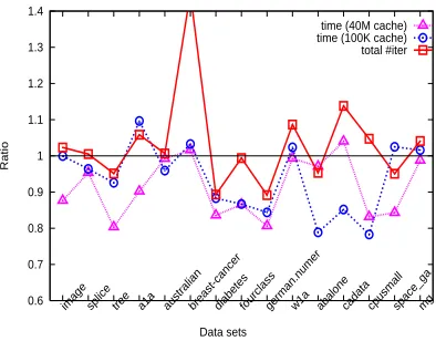
6.2 Experiments
Under the framework WSS 2, we conduct experiments to check if using (11) is really faster than using (33). The same data sets in Section 5 are used under the same setting. For simplicity, we consider only the RBF kernel.
Similar to figures in Section 5, here Figure 9 presents iteration and time ratios between using (11) and (33):
# iter. by using (11) # iter. by using (33),
time by using (11) (100K cache) time by using (33) (100K cache),
time by using (11) (40M cache) time by using (33) (40M cache).
Without shrinking, clearly both approaches have very similar numbers of iterations. This observation is expected due to Theorem 7. Then as (33) costs more than (11) does, the time ratio is in general smaller than one. Especially when the cache is large enough to store all kernel elements, selecting working sets is the main cost and hence the ratio is lower.
With shrinking, in Figures 9(c) and 9(d), the iteration ratio is larger than one for several problems. Surprisingly, the time ratio, especially that of using a small cache, is even smaller than that without shrinking. In other words, (11) better incorporates the shrinking technique than (33) does. To analyze this observation, we check the number of removed variables along iterations, and find that (11) leads to more aggressive shrinking. Then the reduced problem can be stored in the small cache (100K), so kernel evaluations are largely saved. Occasionally the shrinking is too aggressive so some variables are wrongly removed. Then recovering from mistakes causes longer iterations.
Note that our shrinking implementation is by removing bounded elements not in the set (25). Thus, the smaller the interval [M(αk), m(αk)] is, the more variables are shrunk. In Figure 10, we show the relationship between the maximal violationm(αk)−M(αk) and iterations. Clearly using (11) reduces the maximal violation more quickly than using (33). A possible explanation is that (11) has less restriction than (33): In early iterations, if a set B ={i, j}is associated with a large violation−yi∇f(αk)i+yj∇f(αk)j, thendB defined in (15) has large components. Hence though it minimizes the quadratic functions (9),αkB+dB is easily infeasible. To solve (33), one thus changes αkB+dB back to the feasible region as (35) does. As a reduced step is taken, the corresponding Sub(B) may not be smaller than those of using other sets. On the other hand, (11) does not require αkB +dB to be feasible, so a large step is taken. The resulting Sub(B) thus may be small enough so that B is selected. Therefore, using (11) tend to select working sets with large violations and hence may more quickly reduce the maximal violation.
0 5 10 15 20 25
0 10000 20000 30000 40000 50000 60000 70000
(11) (33)
(a)tree
0 0.2 0.4 0.6 0.8 1 1.2 1.4 1.6 1.8
0 200 400 600 800 1000 1200 1400 1600
(11) (33)
(b)splice
0 2 4 6 8 10 12 14
0 1000 2000 3000 4000 5000 6000 7000 8000 9000
(11) (33)
(c)diabetes
0 1 2 3 4 5 6
0 5000 10000 15000 20000 25000 30000
(11) (33)
(d)german.numer
Figure 10: Iterations (x-axis) and maximal violations (y-axis) of using (11) and (33).
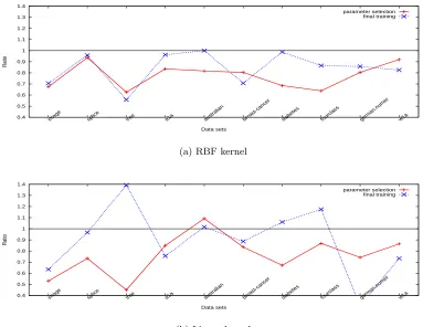
6.3 Sub-problems Using First Order Information
Under first order approximation, we can also modify the sub-problem (8) to the following form, which maintains the feasibility:
Sub(B)≡min
d
B
∇f(αk)T BdB
subject to yBTdB= 0, (43)
0≤αi+di ≤C, i∈B.
Section 2 discusses that a maximal violating pair is an optimal solution of minB:|B|=2Sub(B), where Sub(B) is (8). If (43) is used instead, Simon (2004) has shown an O(l) procedure to obtain a solution. Thus the time complexity is the same as that of using (8).
Note that Theorem 7 does not hold for these two selection methods. In the proof, we use the small changes ofαk
0.4 0.5 0.6 0.7 0.8 0.9 1 1.1 1.2 1.3 1.4
image splice tree a1a australian breast-cancer diabetes fourclass german.numer w1a
Ratio
Data sets
parameter selection final training
(a) RBF kernel
0.4 0.5 0.6 0.7 0.8 0.9 1 1.1 1.2 1.3 1.4
image splice tree a1a australian breast-cancer diabetes fourclass german.numer w1a
Ratio
Data sets
parameter selection final training
(b) Linear kernel
Figure 11: Iteration ratios between using two selection methods: checking all 2l
pairs and WSS 2. Note that the ratio (y-axis) starts from 0.4 but not 0.
7. Discussion and Conclusions
In Section 2, the selection (10) of using second order information may involve checking 2l pairs of indices. This is not practically viable, so in WSS 2 we heuristically fixi∈argm(αk) and examine O(l) sets to find j. It is interesting to see how well this heuristic performs and whether we can make further improvements. By running the same small classification problems used in Section 6, Figure 11 presents the iteration ratio between using two selection methods:
# iter. by Alg. 2 and checking 2l pairs # iter. by Alg. 2 and WSS 2 .
We do not use shrinking and consider both RBF and linear kernels. Figure 11 clearly shows that a full check of all index pairs causes fewer iterations. However, as the average of ratios for various problems is between 0.7 and 0.8, this selection reduces iterations of using WSS 2 by only 20% to 30%. Therefore, WSS 2, an O(l) procedure, successfully returns a working set nearly as good as that by anO(l2) procedure. In other words, theO(l) sets heuristically considered in WSS 2 are among the best in all 2l
Experiments in this paper fully demonstrate that using the proposed WSS 2 (and hence WSS 3) leads to faster convergence (i.e., fewer iterations) than using WSS 1. This result is reasonable as the selection based on second order information better approximates the objective function in each iteration. However, this argument explains only the behavior per iteration, but not the global performance of the decomposition method. A theoretical study showing that the proposed selection leads to better convergence rates is a difficult but interesting future issue.
In summary, we have proposed a new and effective working set selection WSS 3. The SMO-type decomposition method using it asymptotically converges and satisfies other useful theoretical properties. Experiments show that it is better than a commonly used selection WSS 1, in both the training time and iterations.
WSS 3 has replaced WSS 1 in the software LIBSVM(after version 2.8).
Acknowledgments
This work was supported in part by the National Science Council of Taiwan via the grant NSC 93-2213-E-002-030.
Appendix A. WSS 1 Solves Problem (7): the Proof
For any given {i, j}, we can substitute ˆdi ≡ yidi and ˆdj ≡ yjdj to (8), so the objective function becomes
(−yi∇f(αk)i+yj∇f(αk)j) ˆdj. (44)
As di = dj = 0 is feasible for (8), the minimum of (44) is zero or a negative number. If −yi∇f(αk)i >−yj∇f(αk)j, using the condition ˆdi+ ˆdj = 0, the only possibility for (44) to be negative is ˆdj <0 and ˆdi >0. From (3), (8b), and (8c), this corresponds toi∈Iup(αk) and j∈Ilow(αk). Moreover, the minimum occurs at ˆdj =−1 and ˆdi = 1. The situation of −yi∇f(αk)i <−yj∇f(αk)j is similar.
Therefore, solving (7) is essentially the same as
minnmin yi∇f(αk)i−yj∇f(αk)j,0 i∈Iup(αk), j∈Ilow(αk) o
= min −m(αk) +M(αk),0
.
Hence, if there are violating pairs, the maximal one solves (7).
Appendix B. Pseudo Code of Algorithm 2 and WSS 3
B.1 Main Program (Algorithm 2)
Inputs:
y: array of {+1, -1}: class of the i-th instance Q: Q[i][j] = y[i]*y[j]*K[i][j]; K: kernel matrix len: number of instances
eps = 1e-3 // stopping tolerance tau = 1e-12
// main routine
initialize alpha array A to all zero initialize gradient array G to all -1
while (1) {
(i,j) = selectB() if (j == -1)
break
// working set is (i,j)
a = Q[i][i]+Q[j][j]-2*y[i]*y[j]*Q[i][j] if (a <= 0)
a = tau
b = -y[i]*G[i]+y[j]*G[j]
// update alpha
oldAi = A[i], oldAj = A[j] A[i] += y[i]*b/a
A[j] -= y[j]*b/a
// project alpha back to the feasible region sum = y[i]*oldAi+y[j]*oldAj
if A[i] > C A[i] = C if A[i] < 0
A[i] = 0
A[j] = y[j]*(sum-y[i]*A[i]) if A[j] > C
A[j] = C if A[j] < 0
A[j] = 0
A[i] = y[i]*(sum-y[j]*A[j])
// update gradient
deltaAi = A[i] - oldAi, deltaAj = A[j] - oldAj for t = 1 to len
G[t] += Q[t][i]*deltaAi+Q[t][j]*deltaAj }
B.2 Working Set Selection Subroutine (WSS 3)
// return (i,j) procedure selectB
// select i i = -1
if (y[t] == +1 and A[t] < C) or (y[t] == -1 and A[t] > 0) { if (-y[t]*G[t] >= G_max) {
i = t
G_max = -y[t]*G[t] }
} }
// select j j = -1
obj_min = infinity for t = 1 to len {
if (y[t] == +1 and A[t] > 0) or (y[t] == -1 and A[t] < C) { b = G_max + y[t]*G[t]
if (-y[t]*G[t] <= G_min) G_min = -y[t]*G[t] if (b > 0) {
a = Q[i][i]+Q[t][t]-2*y[i]*y[t]*Q[i][t] if (a <= 0)
a = tau
if (-(b*b)/a <= obj_min) { j = t
obj_min = -(b*b)/a }
} } }
if (G_max-G_min < eps) return (-1,-1)
return (i,j) end procedure
References
R. R. Bailey, E. J. Pettit, R. T. Borochoff, M. T. Manry, and X. Jiang. Automatic recog-nition of usgs land use/cover categories using statistical and neural networks classifiers.
In SPIE OE/Aerospace and Remote Sensing, Bellingham, WA, 1993. SPIE.
C. L. Blake and C. J. Merz. UCI repository of machine learning databases. Technical report, University of California, Department of Information and Computer Science, Irvine, CA, 1998. Available at http://www.ics.uci.edu/~mlearn/MLRepository.html.
B. Boser, I. Guyon, and V. Vapnik. A training algorithm for optimal margin classifiers.
In Proceedings of the Fifth Annual Workshop on Computational Learning Theory, pages
Chih-Chung Chang and Chih-Jen Lin. LIBSVM: a library for support vector machines, 2001. Software available at http://www.csie.ntu.edu.tw/~cjlin/libsvm.
Pai-Hsuen Chen, Rong-En Fan, and Chih-Jen Lin. A study on SMO-type decomposition methods for support vector machines. IEEE Transactions on Neural Networks, 2006.
URLhttp://www.csie.ntu.edu.tw/~cjlin/papers/generalSMO.pdf. To appear.
C. Cortes and V. Vapnik. Support-vector network. Machine Learning, 20:273–297, 1995.
Tin Kam Ho and Eugene M. Kleinberg. Building projectable classifiers of arbitrary com-plexity. InProceedings of the 13th International Conference on Pattern Recognition, pages 880–885, Vienna, Austria, August 1996.
Don Hush and Clint Scovel. Polynomial-time decomposition algorithms for support vector machines. Machine Learning, 51:51–71, 2003. URL
http://www.c3.lanl.gov/~dhush/machine_learning/svm_decomp.ps.
Thorsten Joachims. Making large-scale SVM learning practical. In Bernhard Sch¨olkopf, Christopher J. C. Burges, and Alexander J. Smola, editors, Advances in Kernel Methods
- Support Vector Learning, Cambridge, MA, 1998. MIT Press.
S. S. Keerthi, S. K. Shevade, C. Bhattacharyya, and K. R. K. Murthy. Improvements to Platt’s SMO algorithm for SVM classifier design. Neural Computation, 13:637–649, 2001.
D. Lai, N. Mani, and M. Palaniswami. Increasing the step of the Newtonian decomposition method for support vector machines. Technical Report MECSE-29-2003, Dept. Electrical and Computer Systems Engineering Monash University, Australia, 2003a.
D. Lai, N. Mani, and M. Palaniswami. A new method to select working sets for faster training for support vector machines. Technical Report MESCE-30-2003, Dept. Electrical and Computer Systems Engineering Monash University, Australia, 2003b.
Chih-Jen Lin. Linear convergence of a decomposition method for support vector machines. Technical report, Department of Computer Science, National Taiwan University, 2001a.
URLhttp://www.csie.ntu.edu.tw/~cjlin/papers/linearconv.pdf.
Chih-Jen Lin. On the convergence of the decomposition method for support vector machines. IEEE Transactions on Neural Networks, 12(6):1288–1298, 2001b. URL
http://www.csie.ntu.edu.tw/~cjlin/papers/conv.ps.gz.
Chih-Jen Lin. Asymptotic convergence of an SMO algorithm without any as-sumptions. IEEE Transactions on Neural Networks, 13(1):248–250, 2002. URL
http://www.csie.ntu.edu.tw/~cjlin/papers/q2conv.pdf.
D. Michie, D. J. Spiegelhalter, and C. C. Taylor. Machine Learning, Neural and
Sta-tistical Classification. Prentice Hall, Englewood Cliffs, N.J., 1994. Data available at
http://www.ncc.up.pt/liacc/ML/statlog/datasets.html.
Laura Palagi and Marco Sciandrone. On the convergence of a modified version of SVMlight algorithm. Optimization Methods and Software, 20(2-3):315–332, 2005.
J. C. Platt. Fast training of support vector machines using sequential minimal optimiza-tion. In Bernhard Sch¨olkopf, Christopher J. C. Burges, and Alexander J. Smola, editors,
Advances in Kernel Methods - Support Vector Learning, Cambridge, MA, 1998. MIT
Press.
Danil Prokhorov. IJCNN 2001 neural network competition. Slide presentation in IJCNN’01, Ford Research Laboratory, 2001. http://www.geocities.com/ijcnn/nnc_ijcnn01.pdf
.
B. Sch¨olkopf, A. Smola, R. C. Williamson, and P. L. Bartlett. New support vector algo-rithms. Neural Computation, 12:1207–1245, 2000.
Hans Ulrich Simon. On the complexity of working set selection. InProceedings of the 15th