An MDP-Based Recommender System
∗Guy Shani [email protected]
Computer Science Department Ben-Gurion University Beer-Sheva, Israel 84105
David Heckerman [email protected]
Microsoft Research One Microsoft Way Redmond, WA 98052, USA
Ronen I. Brafman [email protected]
Computer Science Department Ben-Gurion University Beer-Sheva, Israel 84105
Editor: Craig Boutilier
Abstract
Typical recommender systems adopt a static view of the recommendation process and treat it as a prediction problem. We argue that it is more appropriate to view the problem of generating recommendations as a sequential optimization problem and, consequently, that Markov decision processes (MDPs) provide a more appropriate model for recommender systems. MDPs introduce two benefits: they take into account the long-term effects of each recommendation and the expected value of each recommendation. To succeed in practice, an MDP-based recommender system must employ a strong initial model, must be solvable quickly, and should not consume too much memory. In this paper, we describe our particular MDP model, its initialization using a predictive model, the solution and update algorithm, and its actual performance on a commercial site. We also describe the particular predictive model we used which outperforms previous models. Our system is one of a small number of commercially deployed recommender systems. As far as we know, it is the first to report experimental analysis conducted on a real commercial site. These results validate the commercial value of recommender systems, and in particular, of our MDP-based approach. Keywords: recommender systems, Markov decision processes, learning, commercial applications
1. Introduction
In many markets, consumers are faced with a wealth of products and information from which they can choose. To alleviate this problem, many web sites attempt to help users by incorporating a
recommender system (Resnick and Varian, 1997) that provides users with a list of items and/or
web-pages that are likely to interest them. Once the user makes her choice, a new list of recommended items is presented. Thus, the recommendation process is a sequential process. Moreover, in many domains, user choices are sequential in nature – for example, we buy a book by the author of a recent book we liked.
The sequential nature of the recommendation process was noticed in the past (Zimdars et al., 2001). Taking this idea one step farther, we suggest that recommendation is not simply a sequential prediction problem, but rather, a sequential decision problem. At each point the Recommender System makes a decision: which recommendation to issue. This decision should take into account the sequential process involved and the optimization criteria suitable for the recommender system, such as the profit generated from selling an item. Thus, we suggest the use of Markov decision processes (MDP) (Puterman, 1994), a well known stochastic model of sequential decisions.
With this view in mind, a more sophisticated approach to recommender systems emerges. First, one can take into account the utility of a particular recommendation – for example, we might want to recommend a product that has a slightly lower probability of being bought, but generates higher profits. Second, we might suggest an item whose immediate reward is lower, but leads to more likely or more profitable rewards in the future.
These considerations are taken into account automatically by any good or optimal policy gen-erated for an MDP model of the recommendation process. In particular, an optimal policy will take into account the likelihood of a recommendation to be accepted by the user, the immediate value to the site of such an acceptance, and the long-term implications of this on the user’s future choices. These considerations are taken with the appropriate balance to ensure the generation of the maximal expected reward stream.
For instance, consider a site selling electronic appliances faced with the option to suggest a video camera with a success probability of 0.5, or a VCR with a probability of 0.6. The site may choose the camera, which is less profitable, because the camera has accessories that are likely to be purchased, whereas the VCR does not. If a video-game console is another option with a smaller success probability, the large profit from the likely future event of selling game cartridges may tip the balance toward this latter choice. Similarly, when the products sold are books, by recommending a book for which there is a sequel, we may increase the likelihood that this sequel will be purchased later.
Indeed, in our implemented system, we observed less obvious instances of such sequential behavior: users who purchased novels by the well-known science fiction author, Roger Zelazny, who uses many mythological themes in his writing, often later purchase books on Greek or Hindu mythology. On the other hand, users who buy mythology books do not appear to buy Roger Zelazny novels afterwards.
The benefits of an MDP-based recommender system discussed above are offset by the fact that the model parameters are unknown. Standard reinforcement learning techniques that learn optimal behaviors will not do – they take considerable time to converge and their initial behavior is random. No commercial site will deploy a system with such behavior. Thus, we must find ways for generating good initial estimates for the MDP parameters. The approach we suggest initializes a predictive model of user behavior using data gathered on the site prior to the implementation of the recommender system. We then use the predictive model to provide initial parameters for the MDP.
Their methods, however, yield poor performance on our data, probably because in our case, due to the relatively limited data set, the use of the enhancement techniques discussed below is needed.
Validating recommender system algorithms is not simple. Most recommender systems, such as dependency networks (Heckerman et al., 2000), are tested on historical data for their predictive accuracy. That is, the system is trained using historical data from sites that do not provide recom-mendations, and tested to see whether the recommendations conform to actual user behavior. We present the results of a similar test with our system showing it to perform better than the previous leading approach.
However, predictive accuracy is not an ideal measure, as it does not test how user behavior is influenced by the system’s suggestions or what percentage of recommendations are accepted by users. To obtain this data, one must employ the system at a real site with real users, and compare the performance of this site with and without the system (or with this and other systems). The extent to which such experiments are possible is limited, as commercial site owners are unlikely to allow experiments which can degrade the performance or the “look-and-feel” of their systems. However, we were able to perform a certain set of experiments using our commercial system at the online bookstore Mitos (www.mitos.co.il) by running two models simultaneously on different users: one based on a predictive model and one based on an MDP model. We were also able, for a short period, to compare user behavior with and without recommendations. These results, which to the best of our knowledge are among the first reports of online performance in a commercial site, are reported in Section 6, providing very encouraging validation to recommender systems in general, and to our sequential optimization approach in particular.
The main contributions of this paper are: (1) A novel approach to recommender systems based on an MDP model together with appropriate initialization and solution techniques. (2) A novel predictive model that outperforms previous predictive models. (3) One of a small number of com-mercial applications based on MDPs. (4) The first (to the best of our knowledge) experimental analysis of a commercially deployed recommender system.
We note that the use of MDPs for recommender systems was previously suggested by Bohnen-berger and Jameson (2001). They used an MDP to model the process of a consumer navigating within an airport. The state of this MDP was the consumer’s position and rewards were obtained when the consumer entered a store or bought an item. Recommendations were issued on a palm-top, suggesting routes and stores to visit. However, the MDP model was hand-coded and experiments were conducted with students rather than real users.
The paper is structured as follows. In Section 2 we review the necessary background on rec-ommender systems, MDPs, and reinforcement learning. In Section 3 we describe the predictive model we constructed whose goal is to accurately predict user behavior in an environment without recommendations. In Section 4 we present our empirical evaluation of the predictive model. In Sec-tion 5 we explain how we use this predictive model as a basis for a more sophisticated MDP-based model for the recommender system. In Section 6 we provide an empirical evaluation of the actual recommender system based on data gathered from our deployed system. We conclude the paper in Section 7 discussing our current and future work.
2. Background
2.1 Recommender Systems
Early in the 1990s, when the Internet became widely used as a source of information, information
explosion became an issue that needed addressing. Many web sites presenting a wide variety of
content (such as articles, news stories, or items to purchase) discovered that users had difficulties finding the items that interested them out of the total selection. Recommender Systems (Resnick and Varian, 1997) help users limit their search by supplying a list of items that might interest a specific user. Different approaches were suggested for supplying meaningful recommendations to users and some were implemented in modern sites (Schafer et al., 2001). Traditional data mining techniques such as association rules were tried at the early stages of the development of recommender systems. Initially, they proved to be insufficient for the task, but more recent attempts have yielded some successful systems (Kitts et al., 2000).
Approaches originating from the field of information retrieval (IR) rely on the content of the items (such as description, category, title, author) and therefore are known as content-based
rec-ommendations (Mooney and Roy, 2000). These methods use some similarity score to match items
based on their content. Based on this score, a list of items similar to the ones the user previously se-lected can be supplied. Knowledge-based recommender systems (Burke, 2000) go one step farther by using deeper knowledge about the user and the domain. In particular, the user is able to introduce explicit information about her preferences. Thus, for instance, the user could specify interest in Thai cuisine, and the system might suggest a restaurant serving some other south-Asian cuisine.
Another possibility is to avoid using information about the content, but rather use historical data gathered from other users in order to make a recommendation. These methods are widely known as collaborative filtering (CF) (Resnick et al., 1994), and we discuss them in more depth below. Finally, some systems try to create hybrid models that combine collaborative filtering and content-based recommendations (Balabanovic and Shoham, 1997; Burke, 2002).
2.2 Collaborative Filtering
The collaborative filtering approach originates in human behavior: people searching for an inter-esting item they know little of, such as a movie to rent at the video store, tend to rely on friends to recommend items they tried and liked. The person asking for advice is using a (small) commu-nity of friends that know her taste and can therefore make good predictions as to whether she will like a certain item. Over the net however, a larger community that can recommend items to our user is available, but the persons in this large community know little or nothing about each other. Conceptually, the goal of a collaborative filtering engine is to identify those users whose taste in items is predictive of the taste of a certain person (usually called a neighborhood), and use their recommendations to construct a list of items interesting for her.
To build a user’s neighborhood, these methods rely on a database of past users interactions with the system. Early systems used explicit ratings. In such systems, users grade items (e.g., 5 stars to a great movie, 1 star to a horrible one) and then receive recommendations.1 Later systems shifted toward implicit ratings. A common approach assumes that people like what they buy. A binary grading method is used when a value of 1 is given to items the user has bought and 0 to other items. Many modern recommender systems successfully implement this approach. Claypool et al. (2001) have suggested the use of other implicit grading methods through a special web browser that keeps track of user behavior such as the time spent looking at the web page, the scrolling of the page by
t Xt−2 Xt−1 Xt
1 – – x1
2 – x1 x2
3 x1 x2 x3 4 x2 x3 x4
Table 1: An auto-regressive transformation of the sequence x1,x2,x3,x4for k=2.
the user, and movements of the mouse over the page. Their evaluation, however, failed to establish a method of rating that gave results consistently better than the binary method mentioned above.
As described in Breese et al. (1998), collaborative filtering systems are either memory based or model based. Memory-based systems work directly with user data. Given the selections of a given user, a memory-based system identifies similar users and makes recommendations based on the items selected by these users. Model-based systems compress such user data into a predictive model. Examples of model-based collaborative filtering systems are Bayesian networks (Breese et al., 1998) and dependency networks (Heckerman et al., 2000). In this paper, we consider model-based systems.
2.3 The Sequential Nature of the Recommendation Process
Most recommender systems work in a sequential manner: they suggest items to the user who can then accept one of the recommendations. At the next stage a new list of recommended items is calculated and presented to the user. This sequential nature of the recommendation process, where at each stage a new list is calculated based on the user’s past ratings, will lead us naturally to our reformulation of the recommendation process as a sequential optimization process.
There is yet another sequential aspect to the recommendation process. Namely, optimal rec-ommendations may depend not only on previous items pruchased, but also on the order in which those items are purchased. Zimdars et al. (2001) recognized this possible dependency and sug-gested the use of an auto-regressive model (a k-order Markov chain) to represent it. They divided a sequence of transactions X1, . . . ,XT (for example, product purchases, web-page views) into cases
(Xt−k, . . . ,Xt−1,Xt) for t=1, . . . ,T as shown in Table 1. They then built a model (in particular, a
dependency network) to predict the last column given the other columns, under the assumption that the cases were exchangeable. Our model will also incorporate this sequential view.
2.4 N-gram Models
N-gram models originate in the field of language modeling. They are used to predict the next
word in a sentence given the last n−1 words. In the simplest form of the model, probabilities for the next word are estimated via maximum likelihood; and many methods exist for improv-ing this simple approach includimprov-ing skippimprov-ing, clusterimprov-ing, and smoothimprov-ing. Skippimprov-ing assumes that the probability of the next word xi depends on words other than just the previous n−1. A
methods that modify the estimates of probabilities to achieve higher accuracy by adjusting zero or low probabilities upward. One type of smoothing is finite mixture modeling, which combines multiple models via a convex combination. In particular, given k component models for xi given
a prior sequence X —pM1(xi|X), . . . ,pMk(xi|X)—we can define the k-component mixture model
p(xi|X) =π1·pM1(xi|X) +· · ·+πk·pMk(xi|X), where∑
k
i=1πi=1 are its mixture weights. Details
of these and other methods are given in Chen and Goodman (1996).
2.5 MDPs
An MDP is a model for sequential stochastic decision problems. As such, it is widely used in applications where an autonomous agent is influencing its surrounding environment through actions (for example, a navigating robot). MDPs (Bellman, 1962) have been known in the literature for quite some time, but due to some fundamental problems discussed below, few commercial applications have been implemented.
An MDP is by definition a four-tuple: hS,A,Rwd,tri, where S is a set of states, A is a set of actions, Rwd is a reward function that assigns a real value to each state/action pair, and tr is the state-transition function, which provides the probability of a transition between every pair of states given each action.
In an MDP, the decision-maker’s goal is to behave so that some function of its reward stream is maximized – typically the average reward or the sum of discounted reward. An optimal solution to the MDP is such a maximizing behavior. Formally, a stationary policy for an MDPπis a mapping from states to actions, specifying which action to perform in each state. Given such an optimal policyπ, at each stage of the decision process, the agent need only establish what state s it is in and execute the action a=π(s).
Various exact and approximate algorithms exist for computing an optimal policy. Below we briefly review the algorithm known as policy-iteration (Howard, 1960), which we use in our imple-mentation. A basic concept in all approaches is that of the value function. The value function of a policyπ, denoted Vπ, assigns to each state s a value which corresponds to the expected infinite-horizon discounted sum of rewards obtained when usingπstarting from s. This function satisfies the following recursive equation:
Vπ(s) =Rwd(s,π(s)) +γ
∑
sj∈S
tr(s,π(s),sj)Vπ(sj) (1)
where 0<γ<1 is the discount factor.2An optimal value function, denoted V∗, assigns to each state
s its value according to an optimal policyπ∗and satisfies
V∗(s) =max
a∈A[Rwd(s,a)) +γs
∑
j∈S
tr(s,a,sj)V∗(sj)]. (2)
To find aπ∗ and V∗ using the policy-iteration algorithm, we search the space of possible poli-cies. We start with an initial policyπ0(s) =argmax
a∈A
Rwd(s,a). At each step we compute the value
function based on the former policy and update the policy given the new value function:
Vi(s) = Rwd(s,πi(s)) +γ
∑
sj∈Str(s,πi(s),sj)Vi(sj), (3)
πi+1(s) = argmax a∈A
[Rwd(s,a) +γ
∑
sj∈S
tr(s,a,sj)Vi(sj)]. (4)
These iterations will converge to an optimal policy (Howard, 1960).
Solving MDPs is known to be a polynomial problem in the number of states (via a reduction to linear programming (Puterman, 1994)). It is usually more natural to represent the problem in terms of states variables, where each state is a possible assignment to these variables and the number of states is hence exponential in the number of state variables. This well known “curse of dimension-ality” makes algorithms based on an explicit representation of the state-space impractical. Thus, a major research effort in the area of MDPs during the last decade has been on computing an optimal policy in a tractable manner using factored representations of the state space and other techniques (for example Boutilier et al. (2000); Koller and Parr (2000)). Unfortunately, these recent methods do not seem applicable in our domain in which the structure of the state space is quite different – that is, each state can be viewed as an assignment to a very small number of variables (three in the typical case) each with very large domains. Moreover, the values of the variables (describing items bought recently) are correlated. However, we were able to exploit the special structure of our state and action spaces using different techniques. In addition, we introduce approximations that exploit the fact that most states – that is, most item sequences – are highly unlikely to occur (a detailed explanation will follow in Section 3).
MDPs extend the simpler Markov chain (MC) model – a well known model of dynamic systems. A Markov chain is simply an MDP without actions. It contains a set of states and a stochastic transition function between states. In both models the next state does not depend on any states other than the current state.
In the context of recommender systems, if we equate actions with recommendations, then an MDP can be used to model user behavior with recommendations – as we show below – whereas an MC can be used to model user behavior without recommendations. Markov chains are also closely related to n-gram models. In a bi-gram model, the choice of the next word depends probabilistically on the previous word only. Thus, a bi-gram is simply a first-order Markov chain whose states correspond to words. An n-gram is a n−1-order Markovian model in which the next state depends on the previous n−1 states. Such variants of MDP-models are well known. A non-first-order Markovian model can be converted into a first-order model by making each state include information related to the previous n−1 states. More general transformation techniques that attempt to reduce the size of the state space have been investigated in the literature (for example, see Bacchus et al. (1996); Thi´ebaux et al. (2002)).
3. The Predictive Model
show that our predictive model outperforms previous models, and in Section 5 we shall intialize our MDP-based recommender system using this predictive model.
3.1 The Basic Model
A Markov chain is a model of system dynamics – in our case, user “dynamics.” To use it, we need to formulate an appropriate notion of a user state and to estimate the state-transition function.
States. The states in our MC model represent the relevant information that we have about the user.
This information corresponds to previous choices made by users in the form of a set of ordered sequences of selections. We ignore data such as age or gender, although it could be beneficial.3 Thus, the set of states contains all possible sequences of user selections. Of course, this formulation leads to an unmanageable state space with the usual associated problems—data sparsity and MDP solution complexity. To reduce the size of the state space, we consider only sequences of at most k items, for some relatively small value of k. We note that this approach is consistent with the intuition that the near history (for example, the current user session) often is more relevant than selections made less recently (for example, past user sessions). These sequences are represented as vectors of size k. In particular, we usehx1, . . . ,xkito denote the state in which the user’s last k selected items
were x1, . . . , xk. Selection sequences with l <k items are transformed into a vector in which x1
through xk−lhave the value missing. The initial state in the Markov chain is the state in which every
entry has the value missing.4 In our experiments, we used values of k ranging from 1 to 5.
The Transition Function. The transition function for our Markov chain describes the
proba-bility that a user whose k recent selections were x1, . . . ,xk will select the item x0 next, denoted trMC(hx1,x2, . . . ,xki,hx2, . . . ,xk,x0i). Initially, this transition function is unknown to us; and we
would like to estimate it based on user data. As mentioned, a maximum-likelihood estimate can be used:
trMC(hx1,x2,x3i,hx2,x3,x4i) =
count(hx1,x2,x3,x4i)
count(hx1,x2,x3i)
(5)
where count(hx1,x2, ...,xki)is the number of times the sequence x1,x2, ...,xk was observed in the
data set. This model, however, still suffers from the problem of data sparsity (for example, see Sarwar et al. (2000a)) and performs poorly in practice. In the next section, we describe several techniques for improving the estimate.
3.2 Some Improvements
We experimented with several enhancements to the maximum-likelihood n-gram model on data different from that used in our formal evaluation. The improvements described and used here are those that were found to work well.
One enhancement is a form of skipping (Chen and Goodman, 1996), and is based on the ob-servation that the occurrence of the sequence x1,x2,x3lends some likelihood to the sequence x1,x3.
That is, if a person bought x1,x2,x3, then it is likely that someone will buy x3after x1. The particular 3. Those user attributes could be incorporated into our model by adding state variables. Attributes with large domains, such as age, can be joined into a (small) number of groups (for example, age groups) to avoid an explosion of the state space. Our similarity and clustering methods (see below) can be adapted to share training data between states with different, but related, attribute values (such as age group 25-30 and age group 30-40).
4. To accommodate systems that collect explicit rather than implicit ratings, each item xi would be replaced by an
skipping model that we found to work well is a simple additive model. First, the count for each state transition is initialized to the number of observed transitions in the data. Then, given a user se-quence x1,x2, ...,xn, we add the fractional count 1/2(j−(i+3))to the transition fromhxi,xi+1,xi+2ito hxi+1,xi+2,xji, for all i+3< j≤n. This fractional count corresponds to a diminishing probability
of skipping a large number of transactions in the sequence. We then normalize the counts to obtain the transition probabilities:
trMC(s,s0) =
count(s,s0) ∑s0count(s,s0)
(6)
where count(s,s0)is the (fractional) count associated with the transition from s to s0.
A second enhancement is a form of clustering that we have not found in the literature. Motivated by properties of our domain, the approach exploits similarity of sequences. For example, the state
hx,y,ziand the statehw,y,ziare similar because some of the items appearing in the former appear in the latter as well. The essence of our approach is that the likelihood of transition from s to s0 can be predicted by occurrences from t to s0, where s and t are similar. In particular, we define the similarity of states si and sj to be
sim(si,sj) = k
∑
m=1δ(smi ,smj)·(m+1) (7)
whereδ(·,·) is the Kronecker delta function and smi is the mth item in state si. This similarity is
arbitrary up to a constant. In addition, we define the similarity count from state s to s0to be
simcount(s,s0) =
∑
si
sim(s,si)·trMCold(si,s0) (8)
where troldMC(si,s0)is the original transition function, with or without skipping (we shall compare the
models created with and without the benefit of skipping). The new transition probability from s0to
s is then given by5
trMC(s,s0) =
1 2tr
old
MC(s,s0) +
1 2
simcount(s,s0) ∑s00simcount(s,s00)
(9)
A third enhancement is the use of finite mixture modeling.6 Similar methods are used in n-gram models, where—for example—a trin-gram, a bin-gram, and a unin-gram are combined into a single model. Our mixture model is motivated by the fact that larger values of k lead to states that are more informative whereas smaller values of k lead to states on which we have more statistics. To balance these conflicting properties, we mix k models, where the ith model looks at the last i transactions. Thus, for k=3, we mix three models that predict the next transaction based on the last transaction, the last two transactions, and the last three transactions. In general, we can learn mixture weights from data. We can even allow the mixture weights to depend on the given case (and informal experiments on our data suggest that such context-specificity would improve predictive accuracy). Nonetheless, for simplicity, we useπ1=· · ·=πk=1/k in our experiments. Because our primary
model is based on the k last items, the generation of the models for smaller values entails little computational overhead.
5. We examined several weighing techniques and the one described yielded the best results. The use of more complex techniques as well as attempts to learn the proper weights resulted in very minor changes.
4. Evaluation of the Predictive Model
Before incorporating our predictive model into an MDP-based recommender system, we evaluated the accuracy of the predictive model. Our evaluation used data corresponding to user behavior on a web site (without recommendation) and employed the evaluation metrics commonly used in the collaborative filtering literature. In Section 6 we evaluate the MDP-based approach using an experimental approach in which recommendations on an e-commerce site are manipulated by our algorithms.
4.1 Data Sets
We base our evaluations on real user transactions from the Israeli online bookstore Mitos (www.mitos.co.il). Two data sets were used: one containing user transactions (purchases) and one containing user browsing paths obtained from web logs. We filtered out items that were bought/visited less than 100 times and users who bought/browsed no more than one item as is commonly done when eval-uating predictive models (for example, Zimdars et al. (2001)). We were left with 116 items and 10820 users in the transactions data set, and 65 items and 6678 users in the browsing data set.7 In our browsing data, no cookies were used by the site. If the same user visited the site with a new IP address, then we would treat her as a new user. Also, activity on the same IP address was attributed to a new user whenever there were no requests for two hours. These data sets were randomly split into a training set (90% of the users) and a test set (10% of the users).
The rational for removing items that were rarely bought is that they cannot be reliably predicted. This is a conservative approach which implies, in practice, that a rarely visited item will not be recommended by the system, at least initially.
We evaluated predictions as follows. For every user sequence t1,t2, ..,tn in the test set, we
generated the following test cases:
ht1i,ht1,t2i, ...,htn−k,tn−k+1, ...,tn−1i (10) closely following tests done by Zimdars et al. (2001). For each case, we then used our various mod-els to determine the probability distribution for tigiven ti−k,ti−k+1, ...,ti−1and ordered the items by
this distribution. Finally, we used the ti actually observed in conjunction with the list of
recom-mended items to compute a score for the list.
4.2 Evaluation Metrics
We used two scores: Recommendation Score (RC) (Microsoft, 2002) and Exponential Decay Score (ED) (Breese et al., 1998) with slight modifications to fit into our sequential domain.
4.2.1 RECOMMENDATIONSCORE
For this measure of accuracy, a recommendation is deemed successful if the observed item ti is
among the top m recommended items (m is varied in the experiments). The score RC is the percent-age of cases in which the prediction is successful. A score of 100 means that the recommendation was successful in all cases. This score is meaningful for commerce sites that require a short list of recommendations and therefore care little about the ordering of the items in the list.
4.2.2 EXPONENTIALDECAYSCORE
This measure of accuracy is based on the position of the observed ti on the recommendation list,
thus evaluating not only the content of the list but also the order of items in it. The underlying assumption is that users are more likely to select a recommendation near the top of the list. In particular, it is assumed that a user will actually see the mth item in the list with probability
p(m) =2−(m−1)/(α−1),(m≥1) (11)
whereα is the half-life parameter—the index of the item in the list with probability 0.5 of being seen. The score is given by
100·∑c∈Cp(m=pos(ti|c))
|C| (12)
where C is the set of all cases, c=ti−k,ti−k+1, ...,ti−1 is a case, and pos(ti|c) is the position of the
observed item ti in the list of recommended items for c. We usedα=5 in our experiments in order
to be consistent with the experiments of Breese et al. (1998) and Zimdars et al. (2001). The relative performance of the models was not sensitive toα.
4.3 Comparison Models
4.3.1 COMMERCESERVER2000 PREDICTOR
A model to which we compared our results is the Predictor tool developed by Microsoft as a part of Microsoft Commerce Server 2000, based on the models of Heckerman et al. (2000). This tool builds dependency-network models in which the local distributions are probabilistic decision trees. We used these models in both a non-sequential and sequential form. These two approaches are described in Heckerman et al. (2000) and Zimdars et al. (2001), respectively. In the non-sequential approach, for every item, a decision tree is built that predicts whether the item will be selected based on whether the remaining items were or were not selected. In the sequential approach, for every item, a decision tree is built that predicts whether the item will be selected next, based on the previous k items that were selected. The predictions are normalized to account for the fact that only one item can be predicted next. Zimdars et al. (2001) also use a “cache” variable, but preliminary experiments showed it to decrease predictive accuracy. Consequently, we did not use the cache variable in our formal evaluation.
These algorithms appear to be the most competitive among published work. The combined results of Breese et al. (1998) and Heckerman et al. (2000) show that (non-sequential) dependency networks are no less accurate than Bayesian-network or clustering models, and about as accurate as Correlation, the most accurate (but computationally expensive) memory-based method. Sarwar et al. (2000b) apply dimensionality reduction techniques to the user rating matrix, but their approach fails to be consistently more accurate than Correlation. Only the sequential algorithm of Zimdars et al. (2001) is more accurate than the non-sequential dependency network to our knowledge.
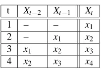
(a) Transactions data set.
(b) Browsing data set.
Figure 1: Exponential decay score for different models.
4.3.2 UNORDEREDMCS
We also evaluated a non-sequential version of our predictive model, where sequences such ashx,y,zi
recom-mendations is incorrect, then we should expect this model to perform better than our MC model, as it learns the probabilities using more training data for each state, gathering all the ordered data into one unordered set. Skipping, clustering, and mixture modeling were included as described in section 2. We call this model UMC (Unordered Markov chain).
(a) Transactions data set.
4.4 Variations of the MC Model
In order to measure how each n-gram enhancement influenced predictive accuracy, we also evalu-ated models that excluded some of the enhancements. In reporting our results, we refer to a model that uses skipping and similarity clustering with the terms SK and SM, respectively. In addition, we use numbers to denote which mixture components are used. Thus, for example, we use MC 123 SK to denote a Markov chain model learned with three mixture components—a bigram, trigram, and quadgram—where each component employs skipping but not clustering.
4.5 Experimental Results
Figure 1(a) and figure 1(b) show the exponential decay score for the best models of each type (Markov chain, Unordered Markov chain, Non-Sequential Predictor model, and Sequential Predic-tor Model). It is important to note that all the MC models using skipping, clustering, and mixture modelling yielded better results than every one of the Predictor-k models and the non-sequential Predictor model. We see that the sequence-sensitive models are better predictors than those that ignore sequence information. Furthermore, the Markov chain predicts best for both data sets.
(b) Browsing data set.
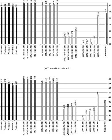
Figure 2: Recommendation score for different models.
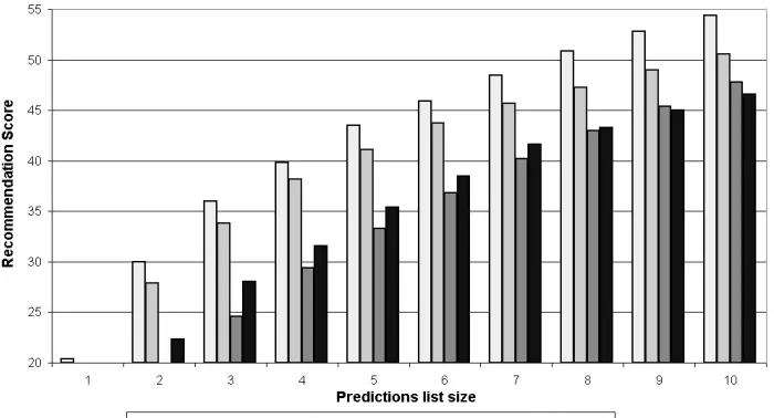
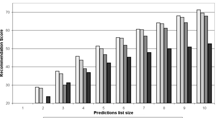
(a) Transactions data set. (b) Browsing data set.
Figure 3: Exponential decay score for different Markov chain versions.
case, once recommendations are available in the site (thus changing the site structure), skipping may prove beneficial.
5. An MDP-Based Recommender Model
The predictive model we described above does not attempt to capture the short and long-term effect of recommendations on the user, nor does it try to optimize its behavior by taking into account such effects. We now move to an MDP model that explicitly models the recommendation process and attempts to optimize it. The predictive model plays an important role in the construction of this model.
We assume that we are given a set of cases describing user behavior within a site that does not provide recommendations, as well as a probabilistic predictive model of a user acting without recommendations generated from this data. The set of cases is needed to support some of the approximations we make, and in particular, the lazy initialization approach we take. The predictive model provides the probability the user will purchase a particular item x given that her sequence of past purchases is x1, . . . ,xk. We denote this value by Prpred(x|x1, . . . ,xk), where k=3 in our case.
It is important to stress that the approach presented here is independent of the particular technique by which the above predictive value is approximated. Naturally, in our implementation we used the predictive model developed in Section 3, but there are other ways of constructing such a model (for example, Zimdars et al. (2001); Kadie et al. (2002)).
5.1 Defining the MDP
Recall that to define an MDP, we need to provide a set of states, actions, transition function, and a reward function. We now describe each of these elements. The states of the MDP for our recom-mender system are k-tuples of items (for example, books, CDs), some prefix of which may contain null values corresponding to missing items. This allows us to model shorter sequences of purchases. The actions of the MDP correspond to a recommendation of an item. One can consider multiple recommendations but, to keep our presentation simple, we start by discussing single recommenda-tions.
Rewards in our MDP encode the utility of selling an item (or showing a web page) as defined by the site. Because the state encodes the list of items purchased, the reward depends on the last item defining the current state only. For example, the reward for statehx1,x2,x3iis the reward generated
by the site from the sale of item x3. In this paper, we use net profit for reward.
The state following each recommendation is determined by the user’s response to that recom-mendation. When we recommend an item x0, the user has three options:
• Accept this recommendation, thus transferring from statehx1,x2,x3iintohx2,x3,x0i
• Select some non-recommended item x00, thus transferring the statehx1,x2,x3iintohx2,x3,x00i. • Select nothing (for example, when the user terminates the session), in which case the system
remains in the same state.
Thus, the stochastic element in our model is the user’s actual choice. The transition function for the MDP model:
is the probability that the user will select item x00 given that item x0 is recommended in state
hx1,x2,x3i. We write trMDP1 to denote that only single item recommendations are used. 5.1.1 INITIALIZINGtrMDP
Proper initialization of the transition function is an important implementation issue in our system. Unlike traditional model-based reinforcement learning algorithms that learn the proper values for the transition function and hence an optimal policy online, our system needs to be fairly accurate when it is first deployed. A for-profit e-commerce8 site is unlikely to use a recommender system that generates irrelevant recommendations for a long period, while waiting for it to converge to an optimal policy. We therefore need to initialize the transition function carefully. We can do so based on any good predictive model, making the following assumptions:
• A recommendation increases the probability that a user will buy an item. This probability is proportional to the probability that the user will buy this item in the absence of recom-mendations. This assumption is made by most collaborative filtering models dealing with e-commerce sites.9 We denote the proportionality constant for recommendation r in state s
byαs,r, whereαs,r>1.
• The probability that a user will buy an item that was not recommended is lower than the probability that she will buy when the system issues no recommendations at all, but still proportional to it. We denote the proportionality constant for recommendation r in state s by βs,r, whereβs,r<1.
To allow for a simpler representation of the equations, for a state s=hx1, ...,xkiand a
recommen-dation r let us use s·r to denote the state s0 =hx2, ...,xk,ri. We use trpredict(s,s·r)to denote the
probability that the user will choose r next, given that its current state is s according to the predictive model in which recommendations are not considered, that is, Prpred(r|s). Thus, withαs,r andβs,r
constant over s and r and equal toαandβ, respectively, we have
tr1MDP(s,r,s·r) =α·trpredict(s,s·r), (14)
the probability that a user will buy r next if it was recommended;
tr1MDP(s,r0,s·r) =β·trpredict(s,s·r),r06=r, (15)
the probability that a user will buy r if something else was recommended; and
trMDP1 (s,r,s) =1−tr1MDP(s,r,s·r)−
∑
r06=rtr1MDP(s,r,s·r0), (16) the probability that a user will not buy any new item after r was recommended. We do not see a reason to stipulate a particular relationship betweenαandβ, although we must have
tr1MDP(s,r,s·r) +
∑
r06=r
tr1MDP(s,r0,s·r)<1. (17)
8. We use the term e-commerce, although our system, and recommender systems in general, can be used in content sites and other applications.
The exact values ofαs,r andβs,rshould be chosen carefully. Choosingαs,r andβs,rto be
con-stants over all states and recommendations (sayα=2,β=0.5) might cause the sum of transition probabilities in the MDP to exceed 1. The approach we took was motivated by Kitts et al. (2000), who showed that the increase in the probability of following a recommendation is large when one recommends items having high lift, defined to be prpr(x(|xh)). Thus, it is not unreasonable to assume that this increase in probability is proportional to lift:
pr(r|s,r)−pr(r|s,r0)∼γp(r|s)
p(r) (18)
where p(r)is the prior probability of buying r. Fixingαs,rto be a little larger than 1 as follows:
αs,r = γ
+p(r)
p(r) (19)
whereγis a very small constant (we useγ= 1
1000), and solving forβs,r, we obtain
βs,r =
1−∑r0αs,r0p(s·r0|s)
(n−1) p(s·r|s) +αs,r. (20) Ifβs,ris negative, we set it to a very small positive value and normalize the probabilities afterwards.
There are a few things to note about tr1MDP(s,r0,s·r), the probability that a user will buy r if something else was recommended, and its representation. First, since tr1MDP(s,r0,s·r) =βs,r·tr(s,s· r), the MDP’s initial transition probability does not depend on r0because our initialization is based on data that was collected without the benefit of recommendations. Of course, if one has access to data that reflects the effect of recommendations (prpredict(s·r|s,r)), one can use it to provide a more
accurate initial model. Next, note that we can represent this transition function concisely using at most two values for every state-item pair: the probability that an item will be selected in a state when it is recommended (that is, pr(s·r|s,r))and the probability that an item will be selected when it is not recommended (that is, pr(s·r|s,r0)). Because the number of items is much smaller than the number of states, we obtain significant reduction in the space requirements of the model.
5.1.2 GENERATINGMULTIPLERECOMMENDATIONS
When moving to multiple recommendations, we make the assumption that recommendations are independent. Namely we assume that for every pair of sets of recommended items, R,R0, we have that
(r∈R∧r∈R0)∨(r∈/R∧r∈/R0) =⇒ trMDP(s,R,s·r) =trMDP(s,R0,s·r) (21)
This assumption might prove to be false. It seems reasonable that, as the list of recommendations grows, the probability of selecting any item decreases. Another more subtle example is the case where the system “thinks” that the user is interested in an inexpensive cooking book. It can then recommend a few very expensive cooking books and one is reasonably priced (but in no way cheap) cooking book. The reasonably priced book will seem like a bargain compared to the expensive ones, thus making the user more likely to buy it.
pair:
trMDP(s,r∈R,s·r) =trMDP1 (s,r,s·r), (22)
the probability that r will be bought if it appeared in the list of recommendations; and
trMDP(s,r∈/R,s·r) =trMDP1 (s,r0,s·r)for all r06=r, (23)
the probability that r will be bought if it did not appear in the list.
As before, trMDP(s,r∈/R,s·r)does not depend on r, and will not depend on R in the discussion
that follows. We note again, that these values are merely reasonable initial values and are adjusted by our system based on actual user behavior, as we shall discuss.
5.2 Solving the MDP
Having defined the MDP, we now consider how to solve it in order to obtain an optimal policy. Such a policy will, in effect, tell us what item to recommend given any sequence of user purchases. For the domains we studied, we found policy iteration (Howard, 1960)—with a few approximations to be described—to be a tractable solution method. In fact, on tests using real data, we found that policy iteration terminates after a few iterations. This stems from the special nature of our state space and the approximations we make, as we now explain.
Our state space enjoys a number of features that lead to fast convergence of the policy iteration algorithm:
Directionality. Transitions in our state space seem to have inherent directionality: First, a state
representing a short sequence cannot follow a state representing a longer sequence. Second, the success of the sequential prediction model indicates that typically, if x is likely to follow y, y is less likely to follow x – otherwise, the sequence x,y and y,x would have similar probabilities, and
we could simply use sets. Thus, loops, which in principle could occur in our MDP model because we maintain only a limited amount of history, are not very likely. Indeed, an examination of the loops in our state space graph reveals them to be small and scarce. Moreover, in the web site implementation, it is easy enough to filter out items that were already bought by the user from our list of recommendations. It is well-known that directionality can be used to reduce the running time of MDP solution algorithm (for example, Bonet and Geffner (2003)).
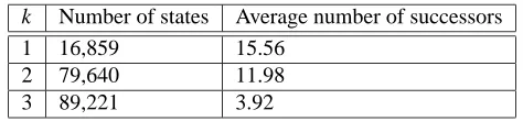
Insensitivity to k. We have also found that the computation of an optimal policy is not
heav-ily sensitive to variations in k—the number of past transactions we encapsulate in a state. As k increases, so does the number of states, but the number of positive entries in our transition matrix remains similar. Note that, at most, a state can have as many successors as there are items. When
k is small, the number of observed successors for a state can be large. When k grows, however, the
number of successors decreases considerably. Table 2 demonstrates this relation in our implemented model.
Despite these properties of the state space, policy evaluation still requires much effort given the large state and action space we have to deal with. To alleviate this problem we resort to a number of approximations.
Ignoring Unobserved States. The vast majority of states in our models do not correspond to
k Number of states Average number of successors
1 16,859 15.56
2 79,640 11.98
3 89,221 3.92
Table 2: The number of initialized states and the average number of state successors for different values of k.
correspond to pairs of states of the form s and s·r. Thus, the number of transitions required per
state is bounded by the number of items rather than by an amount exponential in k in the worst case. The non-zero transitions are stored explicitly, and as can be inferred from Table 2, their number is much smaller than the total number of entries in the explicit transition matrix. And while much memory is still required, in Section 6.2, we show that these requirements are not too large for modern computers to handle.
Moreover, we do not compute a policy choice for a state that was not encountered in our training data. When the value of such a state is needed for the computation of an optimal policy of some observed state, we simply use its immediate reward. That is, if the sequencehx,y,zidid not appear in the training data, we do not calculate a policy for it and assume its value to be R(z)—the reward for the last item in the sequence. Note that given the skipping and clustering methods we use, the probability of making a transition from some (observed) sequence hw,x,yi tohw,x,yi is not zero even thoughhx,y,ziwas never observed. This approximation, although risky in general MDPs, is motivated by the fact that in our initial model, for each state there is a relatively small number of items that are likely to be selected; and the probability of making a transition into an un-encountered state is very low. Moreover, the reward (that is, profit) does not change significantly across different states, so, there are no “hidden treasures” in the future that we could miss.
When a recommendation must be generated for a state that was not encountered in the past, we compute the value of the policy for this state online. This requires us to estimate the transition probabilities for a state that did not appear in our training data. We handle such new states in the same manner that we handled states for which we had sparse data in the initial predictive model – that is, using the techniques of skipping, clustering, and finite mixture of unigram, bigram, and trigrams described in Section 3.2.
Using the Independence of Recommendations. One of the basic steps in policy iteration is
policy determination. At each iteration, we compute the best action for each state s – that is, the action satisfying:
argmax
R
[Rwd(s) +γ∑s0∈Str(s,R,s0)Vi(s0)] =
argmax
R
[Rwd(s) +γ(∑r∈RtrMDP(s,r∈R,s·r)Vi(s·r)+
∑r6∈RtrMDP(s,r∈/R,s·r)Vi(s·r))]
(24)
where tr(s,r∈R,s·r)and tr(s,r∈/R,s·r)follow the definitions above.
independence assumption. Recall that we assumed that the probability that a user buys a particular item depends on her current state, the item, and whether or not this item is recommended. It does not depend on the identity of the other recommended items. The following method uses this fact to quickly generate an optimal set of recommendations for each state.
Let us define∆(s,r)– the additional value of recommending r in state s:
∆(s,r) = (tr(s,r∈R,s·r)−tr(s,r∈/R,s·r))V(s·r). (25)
Now define
Rsmax,κ∆={r1, . . . ,rκ|∆(s,r1)≥. . .≥∆(s,rκ)and
∀r6=ri(i=1, . . . ,κ),∆(s,rκ)≥∆(s,r)}.
(26)
Rsmax,κ∆is the set ofκitems that have the maximal∆(s,r)values.
Theorem 1 Rsmax,κ∆is the set that maximizes Vi+1(s)– that is, Vi+1(s) =
Rwd(s) +γ(∑r∈Rs,κ
max∆tr(s,r∈R,s·r)Vi(s·r)+
∑r∈/Rsmax,κ∆tr(s,r∈/R,s·r)Vi(s·r)).
(27)
Proof Let us assume that there exists some other set ofκrecommendations R6=Rsmax,κ∆ that maxi-mizes Vi+1(s). For simplicity, we shall assume that all∆values are different. If that is not the case,
then R should be a set of recommendations not equivalent to Rsmax,κ∆. Let r be an item in R but not in
Rmaxs,κ∆, and r0be an item in Rmaxs,κ∆but not in R. Let R0be the set we get when we replace r with r0in
R. We need only show that Vi+1(s,R)<Vi+1(s,R0): Vi+1(s,R0)−Vi+1(s,R) =
Rwd(s) +∑s0tr(s,R,s0)Vi(s0)−(Rwd(s) +∑s0tr(s,R0,s0)Vi(s0)) =
∑r00∈Rtr(s,r00∈R,s·r00)Vi(s·r) +∑r00∈/Rtr(s,r00∈/R,s·r00)Vi(s·r00)−
∑r00∈R0tr(s,r00∈R0,s·r00)Vi(s·r)−∑r00∈/R0tr(s,r00∈/R0,s·r00)Vi(s·r00) =
tr(s,r∈R,s·r)Vi(s·r)−tr(s,r0∈/R,s·r0)Vi(s·r0)−
(tr(s,r0∈R0,s·r)Vi(s·r)−tr(s,r∈/R0,s·r0)Vi(s·r)) =
∆(s,r)−∆(s,r0)>0
(28)
To compute Vi+1(s)we therefore need to compute all∆(s,r)and find Rsmax,κ∆, making the
compu-tation of Vi+1(s)independent of the number of subsets (or even worse—ordered subsets) ofκitems.
By construction, our MDP optimizes site profits. In particular, the system does not recommend items that are likely to be bought whether recommended or not, but rather recommends items whose likelihood of being purchased is increased when they are recommended. Nonetheless, when rec-ommendations are based solely on lift, it is possible that many recrec-ommendations will be made for which the absolute probability of a purchase (or click) is small. In this case, if recommendations are seldom followed, users might start ignoring them altogether, making the overall benefit zero. Our model does not capture such effects. One way to remedy this possible problem is to alter the reward function so as to provide a certain immediate reward for the acceptance of a recommenda-tion. Another way to handle this problem is to recommend a book with a large MDP score only if the probability of buying it passes some threshold. We did not find it necessary to introduce these modifications in our current system.
5.3 Updating the Model Online
Once the recommender system is deployed with its initial model, we need to update the model according to actual observations. One approach is to use some form of reinforcement learning— methods that improve the model after each recommendation is made. Although such models need little administration to improve, the implementation requires many calls and computations by the recommender system online, which will lead to slower responses—an undesirable result. A simpler approach is to perform off-line updates at fixed time intervals. The site need only keep track of the recommendations and the user selections and, say, once a week use those statistics to build a new model and replace it with the old one. This is the approach we used.
In order to re-estimate the transition function the following counts are obtained from the recently collected statistics:
• cin(s,r,s·r)—the number of times the r recommendation was accepted in state s.
• cout(s,r,s·r)—the number of times the user took item r in state s even though it was not
recommended,
• ctotal(s,s·r)—the number of times a user took item r while being in state s, regardless of
whether it was recommended or not.
We compute the new counts and the new approximation for the transition function at time t+1 based on the counts and probabilities at time t as follows:
ctin+1(s,r,s·r) = ctin(s,r,s·r) +count(s,r,s·r), (29)
cttotal+1(s,s·r) = cttotal(s,r,s·r) +count(s,s·r), (30)
ctout+1(s,r,s·r) = ctout(s,r,s·r) +count(s,s·r)−count(s,r,s·r), (31)
tr(s,r∈R,s·r) = c
t+1
in (s,r,s·r)
cttotal+1(s,s·r), (32)
tr(s,r∈/R,s·r) = c
t+1
out(s,r,s·r)
cttotal+1(s,s·r). (33)
Note that at this stage the constantsαs,randβs,rno longer play a role—they were used only to
c0in(s,r,s·r) = ξs·tr(s,r,s·r), (34) c0out(s,r,s·r) = ξs·tr(s,r,s·r), (35)
c0total(s,s·r) = ξs, (36)
where ξs is proportional to the number of times the state s was observed in the training data (in
our implementation we used 10·count(s)). This initialization causes states that were observed infrequently to be updated faster than states that were observed frequently and in whose estimated transition probabilities we have more confidence.10
To ensure convergence to an optimal solution, the system must obtain accurate estimates of the transition probabilities. This, in turn, requires that for each state s and for every recommendation
r, we observe the response of users to a recommendation of r in state s sufficiently many times.
If at each state the system always returns the best recommendations only, then most values for
count(s,r,s·r)would be 0, because most items will not appear among the best recommendations. Thus, the system needs to recommend non-optimal items occasionally in order to get counts for those items. This problem is widely known in computational learning as the exploration versus
exploitation tradeoff (for some discussion of learning rate decay and exploration vs. exploitation in
reinforcement learning, see, for example Kaelbling et al. (1996) and Sutton and Barto (1998)). The system balances the need to explore unobserved options in order to improve its model and the desire to exploit the data it has gathered so far in order to get rewards.
One possible solution is to select some constantε, such that recommendations whose expected value isε-close to optimal will be allowed—for example, by following a Boltzmann distribution:
Pr(choose(ri)) =
expV(s·ri)
τ
∑n j=1exp
V(s·rj)
τ
(37)
with an ε cutoff—meaning that only items whose value is within ε of the optimal value will be allowed. The exact value ofεcan be determined by the site operators. The price of such a conser-vative exploration policy is that we are not guaranteed convergence to an optimal policy. Another possible solution is to show the best recommendation on the top of the list, but show items less likely to be purchased as the second and third items on the list. In our implementation we use a list of three recommendations where the first one is always the optimal one, but the second and third items are selected using the Boltzman distribution without a cutoff.
We also had to equip our system to change with frequent changes (for example, addition and removal of items). When new items are added, users will start buying them and positive counts for them will appear. At this stage, our system adds new states for these new items, and the transition function is expanded to express the transitions for these new states. Of course, prior to updating the model, the system is not able to recommend those new items (the well-known “cold start” prob-lem (Good et al., 1999) in recommender systems). In our impprob-lementation, when the first transition to a state s·r is observed, its probability is initialized to 0.9 the probability of the most likely next item in state s withξs=10. This approach causes the new items to be recommended quite frequently.
One possible approach to handling removed items is to do nothing to our system, in which case the transition probabilities slowly decay to zero. Using this approach, however, we may still
insert deleted items into the list of recommended items – an undesirable feature. Consequently, in our Mitos implementation, items are programmatically removed from the model during offline updates. Another solution that we have implemented but not evaluated is to use weighted data and to exponentially decay the weights in time, thus placing more weight on more recently observed transitions.
6. Evaluation of the MDP Recommender Model
The main thesis of this work is that (1) recommendation should be viewed as a sequential optimiza-tion problem, and (2) MDPs provide an adequate model for this view. This is to be contrasted with previous systems which used predictive models for generating recommendations. In this section, we present an empirical validation of our thesis. We compare the performance of our MDP-based recommender system (denoted MDP) with the performance of a recommender system based on our predictive model (denoted MC) as well as other variants.
Our studies were performed on the online book store Mitos (www.mitos.co.il) from August, 2002 till April, 2004. During our evaluations, approximately 5000−6000 different users visited the Mitos site daily. Of those, around 900 users inserted items into their basket, thus entering our data-set.11 On average, each customer inserted 1.97 items into the shopping basket. Over 15,000 items were available for purchase on the site.
Users received recommendations when adding items to the shopping cart.12 The recommen-dations were based on the last k items added to the cart ordered by the time they were added. An example is shown in Figure 4 where the three book covers at the bottom are the recommended items. Every time a user was presented with a list of recommendations on either page, the system stored the recommendations that were presented and recorded whether the user purchased a recommended item. Cart deletions were rare and ignored. Once every two or three weeks, a process was run to update the model given the data that was collected over the latest time period.13
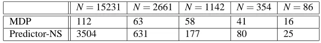
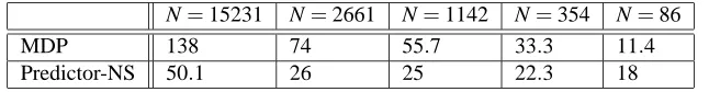
We compared the MDP and MC models both in terms of their value or utility to the site as well as their computational costs.
6.1 Utility Performance
Our first set of results is based on the assumption that the transition function we learn for our MDP using data collected with recommendations, provides the the best available model of user behavior under recommendation. Under this assumption, we can measure the effect of different recommendation policies. An important caveat is that the states in our MDP correspond to truncated (that is, last k) user sequences. Thus, the model does not exclude repeated purchases of the same item. Despite this shortcoming, we proceeded with the evaluation.
As discussed above, a predictive model can answer queries in the form Pr(x|h)—the probability that item x will be purchased given user history h. Recommender systems may employ differ-ent strategies when generating recommendations using such a predictive model. Assuming that an MDP formalizes the recommendation problem well, we may use the learned MDP model to evaluate these strategies. The evaluation of the quality of different possible policies for the MDP, each
corre-11. We do not supply accurate numbers for number of users and actual profits due to the request of the site owners. 12. Users also received recommendations when looking at the description of a book, but these recommendations where
based only on the user’s visit to the current page and not on her cart.
Figure 4: Recommendations in the shopping cart web page.
sponding to a popular approach to recommending, may shed light on the preferred recommendation strategy.
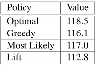
The MDP model was built using data gathered while the model was running in the site with incremental updates (as described above) for almost a year. We compared four policies, where the first policy uses information about the effect of recommendations, and the remaining policies are based on the predictive model solely:
• Optimal – recommends items based on optimal policy for the MDP.
• Greedy – recommends items that maximize Pr(x|h)·R(x)(where Pr(x|h)is the probability of buying item x given user history h, and R(x)is the value of x to the site – for example, net profit).
• Most likely – recommends items that maximize Pr(x|h).
• Lift – recommends items that maximizePrPr(x(x|h)), where Pr(x)is the prior probability of buying item x.
Policy Value
Optimal 118.5 Greedy 116.1 Most Likely 117.0
Lift 112.8
Table 3: Performance of different policies.
The results are presented in Table 3. The calculated value for each policy is the sum of dis-counted profit in (New Israeli Shekels) averaged over all states. We used a weighted average, where the weight of each state was the probability of observing it. Obviously, an optimal policy results in the highest value. However, the differences are small, and it appears that one can use the predictive model alone with very good results.
Next, we performed an experiment to compare the performance of the MDP-based system with that of the MC-based system. In this experiment, each user entering the site was assigned a randomly generated cart-id. Based on the last bit of this cart-id, the user was provided with recommendations by the MDP or MC. Reported mean profits were calculated for each user session (a single visit to the site). Data gathered in both cases was used to update both models.14
The deployed system was built using three mixture components, with history length ranging from one to three for both the MDP model and the MC model. Recommendations from the different mixture components were combined using an equal (0.33) weight. We used the policy-iteration procedure and approximations described in Section 5 to compute an optimal policy for the MDP. Our model encoded approximately 25,000 states in the two top mixture components (k=2, k=3). The reported results were gathered after the model was running in the site with incremental updates (as described above) for almost a year.
During the testing period, 50.7% of the users who made at least one purchase were shown MDP-based recommendations and the other 49.3% of these users were shown MC-based recom-mendations. For each user, we computed the average site profit per session for that user, leaving out of consideration the first purchase made in each session. The first item was excluded as it was bought without the benefit of recommendations, and is therefore irrelevant to the comparison between the recommender systems.15
The average site profit generated by the users was 28% higher for the MDP group.16 We used a permutation test (see, for example, Yeh (2000)) to see how likely it would be for a difference this large to emerge if there were in fact no systematic difference in the effectiveness of the two recommendation methods.17 We randomly generated 10000 permutations of the assignments of
14. We update the MC model by recording the transition without considering the recommendation used.
15. This is not entirely accurate as the site also provides recommendations for items in the book description page. We do not present here any experimental results for those recommendations and do not model their effect on the user, but we note that a user that received MDP recommendations in the cart page, got MDP recommendations in the book description page; users who got MC recommendations in the basket got MC recommendations in the description page as well.
16. We are not at liberty to provide accurate numbers.