http://www.sciencepublishinggroup.com/j/ajtas doi: 10.11648/j.ajtas.20180706.17
ISSN: 2326-8999 (Print); ISSN: 2326-9006 (Online)
Methodology Article
Using Excel to Simulate and Visualize Conditional
Heteroskedastic Models
William Henry Laverty
1, Ivan William Kelly
21Department of Mathematics and Statistics, University of Saskatchewan, Saskatoon, Canada
2Department of Educational Psychology & Special Education, University of Saskatchewan, Saskatoon, Canada
Email address:
To cite this article:
William Henry Laverty, Ivan William Kelly. Using Excel to Simulate and Visualize Conditional Heteroskedastic Models. American Journal of
Theoretical and Applied Statistics. Vol. 7, No. 6, 2018, pp. 242-246. doi: 10.11648/j.ajtas.20180706.17
Received: October 29, 2018; Accepted: November 21, 2018; Published: December 18, 2018
Abstract:
Longitudinal data are available in many disciplines, and quite often the mechanism generating the data are changing over time. These changes must be accounted for when modelling the data and subsequently drawing conclusions from the data. The three statistical models described in this article (GARCH, HMM, ARHMM) are appropriate modelling data with such changes. These three models are generalizations of a random walk. In a random walk the random changes over time have a constant distribution. The three models illustrated account for changes in the distribution of the random displacements over time. Our purpose in the article is to illustrate these three models and their intricacies using Excel. We would also contend and encourage the application of these three models to the analysis of other continuous data in fields utilizing social and medical data.Keywords:
Time Series Analysis, GARCH, Hidden Markov Models (HMM), Autoregressive Hidden Markov (ARHMM), Simulation, Excel1. Introduction
In 1973, the book ‘A Random Walk Down Wall Street’ [1] popularized the idea that the stock market followed a random walk. A Random Walk is a stochastic process consisting of series of steps generated by chance. In its simplest form the steps are coming from a common distribution (usually Normal with mean 0 and a fixed standard deviation. Since then, more advanced statistical models which allowed for heteroskedasticity of stock market jumps incorporated in the modeled random walks have become common in financial research. Such statistical refinements are necessary when trading in financial options. The underlying parameters (mean and variance of the random jumps) that generate data from a random walk collected over time can change over time. It is important for the models of such data to reflect these changes. If it is only the mean that is changing, this has been traditionally handled by fitting polynomial regression models, trigonometric polynomial regression models and exponential decay models or combinations thereof. Data collected over time is also likely to be serially correlated (present
observations correlated with past observations). Such data has been modelled by the traditional Box-Jenkins models (ARMA, ARIMA etc). In Box-Jenkins models (ARMA, ARIMA) the white noise component that is driving these models is assumed to have a constant variance. Sometimes this is not true leading to Conditional Heteroscedastic Models, which do not make this assumption [2]. The variance of the random jumps can change over time for example with financial data in more volatile periods. This leads to the common use of the Conditional Heteroskedastic models such as the GARCH and HMM models. If in addition the serial auto correlation changes during differing periods of time an ARHMM model becomes applicable. The purpose of this paper is to illustrate various Conditional Heteroskedastic Models by simulating data from these models using Excel similar to that in Laverty, Miket and Kelly [3].
2. Conditional Heteroscedastic Models
2.1. The GARCH(m, s) Model
could also be applied to social data [4]. The random walk model where steps are assumed to be independent mean zero common variance has been previously widely used as models for financial data. On the other hand, the assumption of constant variance appears often not to hold true. In the GARCH models the variance is not assumed to be constant but evolving over time and depending on past values of the variance and previous observations in the process. Namely if {u
t} represent random jumps in a financial process then a
GARCH(m, s) model is described by
, ∑ ∑ (1)
where { zt} are independent identically distributed (iid) variables with mean zero, variance one. where { u
t} are
independent identically distributed (iid) variables with mean zero variance
with 0, 0, 0 and
!"# , $
%$ & 1 Simulation of a GARCH Model with Normal Observations in Excel
Figure 1. GARCH Random Walk.
Uniform random variates on [0,1] can be generated in Excel with the function “RAND()”. The generation of random variates with a Normal distribution with mean µ and standard deviation σ, can be carried out using the inverse-transform method [5]. Namely Y = F-1(U) where F(u) is the desired cumulative distribution of Y and U has a uniform distribution on [0,1]. In Excel this is achieved for the Normal distribution (mean µ, standard deviation σ) with the function “NORMINV(RAND(),µ,σ).”
To simulate a GARCH(2, 2) model with normal observations with mean 0 and parameters φ0, φ1, φ2, θ1 and θ2. Place the values of these parameters in the cells G1, G2, G3, J2 and J3. Place the values of time (t = 1, … , 200) in cells A18:A217. The values of zt are calculated by the
formula, “=NORMSINV(RAND())” , in cells E18:E217. The values of are computed by placing the formula “=G$1+G$2*(B16^2)+G$3*(B15^2)+J$2*D15+J$3*D 16” in cell D18 and copying it down to Cell D217.
The values of are computed by placing in cell C18 the formula
“=SQRT(D18)” and copying it down to Cell C217. Finally the values of are computed by placing in cell B18 the formula
“=C18*E18” and copying it down to Cell B217.
A random walk with changes modeled by { : 1 ) * ) 200, is achieved by placing formula “=100+B18” in cell F18 and formula “=F18+B19” in cell F19. Then the formula in cell F19 is copied down to cell F217.
2.2. The Hidden Markov Model (HMM)
Hidden Markov models (HMMs) are a widely used collection of statistical models. These models are applicable when studying a process that goes through a sequence of states. These states are unseen (hidden) but what is observed is data from each state. For example HMMs have been used to model heart rate variability [6], to model financial data [7], to model residuals in regression [8, 9] and Real-Time Spam Tweets Filtering [10] .
A hidden Markov model will consist of a sequence of states X1, X2,…, XT, together with a sequence of observations Y1,
Y2,…, YT. We assume that the number of states (possible
values of each Xi) is a finite number, m. The states can be
represented by the integers 1, 2, ..., m. The states are not observed. The observations Y1, Y2,…, YT are observed and
could be vectors of dimension k. In this paper k = 1. The distribution of Yt depends on the state Xt, the state the
assuming that there are only two states and that the distribution of Yt if Xt = i (i = 1, 2) is the Normal
distribution with mean µi and standard deviation σi.
The parameters of the hidden Markov model are the initial state probabilities,
πi= Pr(X1 = i ) i = ,2, …, m (2) and the transition probability matrix Γ= (γij). This is an m x
m matrix, with element γij being the probability of a
transition into state j starting from state i. i.e.
γij = Pr(Xt = jl Xt-1 = i ), (3) where t denotes time. These two choices allow us to construct a sequence of states (known also as the Markov chain) X1,
X2, . . ., XT constituting the hidden part of a hidden Markov
model.
When the Markov chain is in state i, at time t,it emits an observed signal Yt, which is either a discrete or a continuous
random variable (or random vector) with distribution conditional on the current state i.
In the discrete case
Pr [Yt = y| Xt = i] = pi(y;θi) (4)
where pi is probability mass function with parameters θi.
In the continuous case the conditional density of Yt= y
given Xt= i is fi(y;θi)
In this paper we will assume that fi(y;θi) is the Normal
distribution with mean µi and standard deviation σi.
Simulation of a Hidden Markov Model with Normal Observations in Excel
To simulate a Hidden Markov model with m = 2 states and normal observations with mean µi and standard
deviation σiwhen the Markov process is in state i we to first
need to determine the sequence of states then generate the observations from those states.
Initially we will store the parameters of the model in various cells of the excel spread sheet. For example, the transition probabilities γij(i = 1,2; j = 1,2) will be stored in
the cells B3:C4, the initial probabilities πi (i = 1,2) will
stored in cells B9:C9, and the parameters of the normal distribution (µi, σi) i = 1, 2 will be stored in cells H3:I4. The
next step is to generate the sequence of states. We generate the first state by determining if a uniform random variate U is above or below π1. This is achieved by placing the formula “IF(RAND()<B9,1,2)” in cell C13. We now generate the following sequence of states determining if a uniform random variate U is above or below γi1. This is achieved by placing the formula “IF(OR(AND(C13=1, RAND()<B$3), AND(C13=2, RAND()<B$4)),1,2)” in cell C14. This formula can now be copied down to generate as many states as desired (In this paper we generate 200 states and observations). The final step is to generate normal observations with mean µiand standard deviation σiat each
time point when the process is in state i. This is achieved by pasting the formula “IF(C13=1, H$3+I$3*NORMSINV(RAND()),
H$4+I$4*NORMSINV(RAND()))” into cell B13. Again this formula can now be copied down to generate the complete set of data.
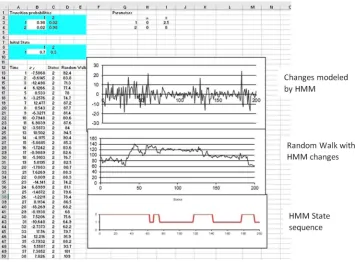
A random walk with changes modeled by { : 1 ) * ) 200, is achieved by placing formula “=100+B12” in cell D12 and formula “=D12+B13” in cell D13. Then the formula in cell D13 is copied down to cell D211.
Below is a copy of the spreadsheet with graphs of the data sequence and the state sequence and the random walk generated by the data sequence.
2.3. The ARHMM Model
Many applications of Hidden Markov Models are possible whenever we have data collected over time. The traditional time series models (AR, MA, ARMA etc.) assume that the process generating the data is constant over a single state. However, if the data is observed over longer periods of time it is likely that there are changes in the states that are generating the data. In the Hidden Markov Model the observations could be assumed to be independent when the state is constant. Alternatively, when the state is constant one could assume that that observations are correlated in the same way that an autoregressive (AR) time series is correlated. This leads to the Autoregressive Hidden Markov (ARHMM) model described in [11], [12] and [13].
Simulation of an Autoregressive Hidden Markov Model with Normal Observations in Excel
To simulate an Autoregressive Hidden Markov model with m = 2 states and normal observations with mean µi,
standard deviation σI and autoregressive parameter βiwhen
the Markov process is in state i we again need to determine the sequence of states and then generate the observations from those states.
Initially we will store the parameters of the model in various cells of the excel spread sheet. For example, the transition probabilities γij(i = 1,2; j = 1,2) will be stored in
the cells B3:C4, the initial probabilities πi (i = 1,2) will
stored in cells B9:C9, and the parameters of ARHMM the normal distribution (µi, σi, βi) i = 1, 2 will be stored in cells
H3:J4.
The next step is to generate the sequence of states. We generate the first state by determining if a uniform random variate U is above or below π1. This is achieved by placing the formula “IF(RAND()<B9,1,2)” in cell C13. We now generate the following sequence of states determining if a
uniform random variate U is above or below γi1. This is achieved by placing the formula “IF(OR(AND(C13=1, RAND()<B$3), AND(C13=2, RAND()<B$4)),1,2)” in cell C14. This formula can now be copied down to generate as many states as desired (In this paper we generate 200 states and observations). The final step is to generate normal observations with mean - . /0123 45
65 7and standard deviation σi at each time point, t, when the process is in
state i at time t and state j at time t – 1. To obtain an observation with the above properties we would compute 8 - . /0123 45
65 7 where is a N(0,1) random variate. This is achieved by pasting the formula
“=VLOOKUP(C14, G$4:H$5,2)
+VLOOKUP(C14, G$4:J$5,4)*(B13-VLOOKUP(C13, G$4:H$5,2))/VLOOKUP(C13, G$4:I$5,3)
+VLOOKUP(C14, G$4:I$5,3)*NORMSINV(RAND())”
into cell B13.
Note: VLOOKUP(C14, G$4:H$5,2) obtains the value -VLOOKUP(C13, G$4:H$5,2) obtains the value -VLOOKUP(C14, G$4:I$5,3) obtains the value VLOOKUP(C13, G$4:I$5,3) obtains the value , and VLOOKUP(C14, G$4:J$5,4) obtains the value ..
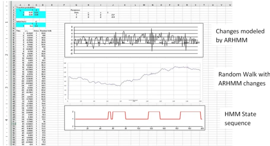
Again, this formula can now be copied down to generate the complete set of data. Below is a copy of the spreadsheet with graphs of the data sequence and the state sequence.
A random walk with changes modeled by { : 1 ) * ) 200, is achieved by placing formula “=100+B12” in cell D12 and formula “=D12+B13” in cell D13. Then the formula in cell D13 is copied down to cell D211.
Below is a copy of the spreadsheet with graphs of the data sequence and the state sequence and the random walk generated by the data sequence.
3. Conclusion
In this article we have illustrated, using EXCEL, the simulation of random walks based GARCH, HMM and ARHMM models. This allows the reader to observe and compare realizations of these models. We believe that these models can apply to longitudinal data in other areas such as the Social Sciences, neurological data, and medicine. For example, there may be periods (states) of higher and lower volatility not incorporated into traditional regression analyses. In medicine, states of increasing variability may indicate serious changes in patient’s well-being---and these would be uncovered by models such as GARCH.
References
[1] B. G. Malkiel (1973) A Random Walk Down Wall Street. W. W. Norton. New York (NY).
[2] R. S. Tsay (2010) Analysis of Financial Time Series. Third Edition. Wiley. Hoboken (NJ).
[3] W. H. Laverty, M. J. Miket, and I. W. Kelly. (2002). Simulation of Hidden Markov Models with EXCEL, Journal of Royal Statistical Society. Series D. 51: 31-40.
[4] I. Visser, M. E. J Raijmakers and P. C. M Molenaar (2002) Fitting Hidden Markov Models to psychological data. Scientific Programming. 10: 185-199. DOI: 10.1109/ICMEW.2013.6618397.
[5] G. S. Fishman (1995) Monte Carlo, Concepts, Algorithms and Applications. Springer, NewYork (NY).
[6] M. Walker II, (2011) Hidden Markov Models for Heart Rate Variability with Biometric Applications. All Theses and Dissertations (ETDs). 491.
[7] R. Mamon, Elliott. (2007) Hidden Markov Models in Finance. International Series n Operations Research and Management Science. Springer. New York. (NY).
[8] W. H. Laverty, M. J. Miket, and I. W. Kelly IW. (2002) Application of Hidden Markov Models on residuals: an example using Canadian traffic accident data. Perceptual and Motor Skills. 94(3 Pt 2): 1151-6.
[9] W. H. Laverty, M. J. Miket, and I. W. Kelly. (2002) Examination of Residuals to Vancouver Crisis Call Data by using Hidden Markov Models. Perceptual and Motor Skills. 94: 548-550.
[10] M. Washha, A. Qaroush, M. Mezghani, and F. Sedes (2017) A Topic-Based Hidden Markov Model for Real-Time Spam Tweets Filtering. 21st International Conference on Knowledge Based and Intelligent Information and Engineering Systems, 6-8 September, Marseille, France.
[11] B. H. Juang & L. R. Rabiner (1986) Mixture autoregressive hidden Markov models for speech signal, IEEE Transactions on Acoustics Speech and Signal Processing. 33(6): 1404 – 1413.
[12] X. Tang. (2004). Autoregressive Hidden Markov Model with Application in an El Nin ̃o study. Master’s thesis, University of Saskatchewan, Saskatoon, Saskatchewan, Canada.