Modeling the Epidemiology of Malaria and Control with Estimate of the Basic Repro-duction Number

(1)

Published online February 20, 2013 (http://www.sciencepublishinggroup.com/j/pamj) doi: 10.11648/j.pamj.20130201.17

Modeling the epidemiology of malaria and control with

estimate of the basic reproduction number

Adamu Abdul Kareem

1

, Anande Richard Kimbir

2

1

Mathematical Sciences Department, School of Pure & Applied Sciences, Modibbo Adama University of Technology Yola, Adamawa State, Nigeria

2

Department of Mathematics & Computer, University of Agriculture, Markudi, Benue State, Nigeria

Email address:

[email protected] (A. A. Kareem) , [email protected] (A. R. Kimbir)

To cite this article:

Adamu Abdul Kareem, Anande Richard Kimbir. Modeling the Epidemiology of Malaria and Control with Estimate of the Basic Repro-duction Number, Pure and Applied Mathematics Journal. Vol. 2, No. 1, 2013, pp. 42-50. doi: 10.11648/j.pamj.20130201.17

Abstract:

Strategies for controlling the epidemiology of many infectious diseases such as malaria include a rapid reduc-tion in both the infected and susceptible populareduc-tion via treatment and vaccinareduc-tion. In this paper, we have modified the Tumwiine et al. (2007) mathematical model for the transmission of malaria by including a vaccination parameter. We have shown that the model has a unique disease-free equilibrium state which is locally and globally asymptotically stable, if

R

_o

≤

1, and that the endemic equilibrium exist provided

R

_o

> 1, where o

R

is a parameter which depends on the given mod-el parameters. Numerical simulations of the modified modmod-el clearly show that, with a proper combination of treatment and vaccination, offered at about 65% each on the susceptible and infected population, malaria can be eradicated from the community.

Keyword:

Malaria, Disease-Free Equilibrium Point, Reproduction Number, Endemic Equilibrium Point, Global Asymp-totical Stability, Lyaponuv Function

1. Introduction

Malaria is the common name for diseases caused by sin-gle-celled parasites of the genus Plasmodium. Among the parasites of the genus Plasmodium four species have been identified which can cause disease in humans. These in-clude: Plasmodium falciparum, Plasmodium vivax, Plas-modium malaria and PlasPlas-modium ovale. Of these, Plasmo-dium falciparum is of greatest risk to non-immune humans. The Plasmodium falciparum variety of parasites account for 80% of cases and 90% off deaths (Kakkilaya, 2003).Malaria remains arguably the greatest menace of our society in terms of morbidity and mortality and the occur-rence of malaria in our part of the world correlates with poverty, ignorance and social deprivations in the communi-ty. An accurate knowledge of the incidence of malaria in endemic areas would be necessary towards the planning and development of effective preventive measures against the deadly scourge of malaria. Malaria is spread by the bite of an infected female mosquito, of the genus anopheles each time the infected insect takes a blood meal. The symp-toms in an infected human include bouts of fever, headache,

vomiting flu-like, anemia (destroying red blood cell) and malaria can kill by clogging the capillaries that carry blood to the brain (cerebral malaria) or other vital organs. On the average the incubation period of Plasmodium falciparum is about 12 days in humans. Malaria is endemic to tropical areas where the climatic and weather conditions allow con-tinuous breeding of the mosquito. Malaria is one of the most important parasitic and infectious diseases especially in tropical and subtropical areas caused by protozoan para-sites of the genus plasmodium. Malaria, affecting mainly children and pregnant women is one of the greatest menac-es of our society in terms of morbidity and mortality and the occurrence of malaria in our part of the world correlates with poverty and ignorance (Perandin, 2003). Malaria is a major public health problem in the world. The WHO esti-mates that in tropical countries among the 500 million cas-es of malaria infection, one million deaths occur annually.

(2)

human-pathogenic Plasmodium species is usually referred to as malaria parasites The parasites multiply within red blood cells, causing symptoms that include symptoms of anaemia, as well as other general symptoms such as fever, chills, nausea, flu-like illness, and in severe cases, coma and death (Deressa et al., 2000). It is a disease that can be treated in just 48 hours, yet it can cause fatal complications if the diagnosis and treatment are delayed.

2. Role of Mathematical Model

It is important to establish the transmission dynamics of an epidemic in order to understand and predict it. Mathe-matical models are particularly helpful as experimental tools with which to evaluate and compare control proce-dures and preventive strategies, and to investigate the rela-tive effects of various sociological, biological and envi-ronmental factors on the spread of diseases. These models have played a very important role in the history and devel-opment of vector-host epidemiology. Several authors have used mathematical models to analyse the transmission and spread of malaria. Mathematical models of malaria trans-mission that include both mosquito and human populations have been reviewed and discussed in detail by various au-thors. Nedelman (1985), did some further work on malaria model of Dietz et al. (1974), and showed that the “vaccina-tion” rate depends on a pseudoequilibrium approximation to the differential equation describing the mosquito dynam-ics in the malaria model. Nedelman surveys various data sets to statistically approximate parameters such as inocu-lation rates, rates of recovery and loss of immunity in hu-mans, human-biting rates of mosquitoes and infectivity and susceptibility of humans and mosquitoes. Dietz et al. (1974) proposed a model with two different classes of humans: one without immunity to malaria and one class with some immunity. As the non-immune class falls sick, some people recover with immunity. The immune class can get infected, but does not fall clinically ill and cannot be infectious. The model by Dietz et al. (1974) also included super infection, a phenomenon usually associated with macro parasites.

Yang (2000) describes a compartmental model where humans follow an SEIRS-type (with more than one im-mune class for humans) pattern and mosquitoes follow a Susceptible-Exposed-Infectious (SEI) pattern. Yang (2000) defines a reproductive number,

R

O_{for this model and} shows, through linear stability analysis, that the disease-free equilibrium is stable for

R

O_{< 1. He also derived an} expression for an endemic equilibrium that is biologically relevant only when

R

O_{> 1. He used numerical} simula-tions to support his proposition that for

R

O_{> 1, the} dis-ease-free equilibrium is unstable and the endemic equili-brium is stable. The model for malaria transmission that we modified is an extension of the equations introduced by Tunwiine et al. (2007). In the Tunwiine model, humans follow an SIRS-like pattern and mosquitoes follow a SI pattern, similar to that described by Yang (2000) but with only one immune class for humans. Humans move from

the susceptible to the infected class at some probability when they come into contact with an infectious mosquito, as in conventional SIRS models. However, infectious people can then recover with, or without, a gain in immuni-ty; and either return to the susceptible class, or move to the recovered class. A new feature of this model is that al-though individuals in the recovered class are assumed to be “immune”, in the sense that they do not suffer from serious illness and do not contract clinical malaria, they still have low levels of Plasmodium in their blood stream and can pass the infection to susceptible mosquitoes. After some period of time these recovered individuals return to the susceptible class. Susceptible mosquitoes get infected and move to the infected class, at some probability when they come into contact with either infectious humans or recov-ered humans (albeit at a much lower probability). Both humans and mosquitoes leave the population through a density dependent natural death rate. This allows the model to account for changing human and mosquito populations. Variations in mosquito populations are crucial to the dy-namics of malaria, and constant population models do not account for this. The model also includes human disease-induced death as mortality for malaria in areas of high transmission can be high, especially in infants. In the mod-ified model, we aim to capture some of the more important aspects of this epidemiology while still keeping it mathe-matically tractable. One of the major important factors that we include in the existing model is vaccination in order to determine its impact as a control measure for the spread of malaria.

2.1. Parameters and Terms of the Model

H

S

(t) the number of susceptible human host at time t

H

I

(t) the number of infected human host at time t

H

R

(t) the number of partially immune human host at-time t

V

S

(t) the number of susceptible mosquito vector at time t

V

I

(t) the number of infected mosquito vectors at time t

H V

N N

m = _{the number of female mosquitoes per human}

host

a the average daily biting rate on man by a single mos-quito (infection rate)

b the proportion of bites on man by a single mosquito that produce an infection

c the probability that a mosquito becomes infectious

γ

the per capita rate of loss of immunity in human host r the rate at which human host acquire immunity

δ

the per capita death rate of infected human hosts due to the disease

v the rate of recovery of human host from the disease

h

λ

the per capita natural birth rate of humans

v

(3)

h

µ

the per capita natural death rate of humans

v

µ

the per capita natural death rate of the mosquitoes

α

the ‘vaccination rate’ on human

3. Equations of the Model

The model formulated by Tumwiine et al. (2007) is giv-ing as H h H H H V H H h H S R vI N I abS N dt

dS

_λ

_γ

_µ

− + + −

= (3.1)

H h H H H H V H H I I rI vI N I abS dt

dI _δ _µ

− − − −

= (3.2)

H h H H

H

_rI

_R

dt

dR

µ

γ

−

=

(3.3)

V v H H V V v V

_S

N

I

acS

N

dt

dS

µ

λ

−

=

(3.4)

V v H H V V

_I

N

I

acS

dt

dI

µ

−

=

(3.5)

We assumed that all infected human who recovered are moved to the recovered class and vaccinated human have temporary immunity that expires over time and again be-come susceptible, hence by including a vaccination para-meter, “

α

” the above model gives the modified model below H H h H H V H H h

H

_R

_S

N

I

abS

N

dt

dS

α

µ

γ

λ

−

+

−

=

(3.6)

H h H H H V H

H

_rI

_I

N

I

abS

dt

dI

µ

δ

−

=

(3.7)

H H h H H H

S

R

rI

dt

dR

α

µ

γ

−

+

−

=

(3.8)

V v H H V V v V

S

N

I

acS

N

dt

dS

µ

λ

−

=

(3.9)

V v H H V V

_I

N

I

acS

dt

dI

µ

−

=

(3.10)

The total population sizes

N

_H and

N

_V can be deter-mined by

S

_H+

I

_H+

R

_H=

N

_H and

S

_V+

I

_V=

N

_V or from the differential equations

H H h h

H _N _I

dt dN

δ

µ

λ

− −

=( ) (3.11)

and V V V V _N dt dN ) (λ − µ

= (3.12)

which are derived by adding equation (3.6) – (3.8) for the human population and (3.9) – (3.10) for the mosquito vector population.

In the model, the term H V H N I abS

denotes the rate at which

the human hosts

S

_Hget infected by infected mosquitoes

V

I

and H H V N I acS

refers to the rate at which the susceptible

mosquitoes

S

_Vare infected by infected human hosts

I

_H.

3.1. Existence and Stability of Equilibrium Solutions

In this section, we establish that the disease free equili-brium

E

_oexists if

R

_O<1. We also establish that the en-demic equilibrium

E

_E exist for

R

_O>1.

Setting equation R.H.S of equation (3.6) - (3.10) to zero gives the disease equilibrium points:

O

E

=

(

S

_Ho

,

I

_Ho

,

R

_Ho

,

S

_Vo

,

I

_Vo

)

=

(

)

(

)

(

)













+

0 ,

,

0 ,

v V v h h H h h h h H

h

N

µ

λ

α

γ

µ

α

λ

α

γ

µ

γ

µ

λ

The disease-free equilibrium Eoexists for all nonnega-tive values of its parameters.

At the steady states of the model, the Jacobian matrix at

E is given by

E

J

= v H H H V v H H H V h H H h H V H H h H V N acI N acS N acI N acS r N abS r N abI N abS N abI µ µ µ γ α µ δ γ α µ − − − − − − − − − − − − − 0 0 0 0 0 0 0 0 0 0 0 (3.13)

Evaluating the Jacobian matrix at

E

_O gives

O E

J

= ( ) ( ) ( ) ( ) v v H V v v v H V v h h h h H h H h h h h H h H h N N ac N N ac r N N ab r N N ab µ µ λ µ µ

λ γ µ

α µ µ α γ

µ γ λ µ δ γ α µ µ µ γ λ γ α µ − − − − − + + +       − − − + + +      ₋ − − 0 0 0 0 0 0 0 0 0 0 0 0 0 (3.14)

The stability of the disease free equilibrium state can be obtained from studying the eigenvalues of

O

E

(4)

points are locally asymptotically stable. The five eigenvalues of

J

_E_O are

h

µ

λ

1

=

4

=

−

<0

(

B C

)

K− +

=

2

λ . This may be either nega-tive or positive

(

B

C

)

K

+

−

=

3

λ

<0

γ

α

µ

λ

5

=

−

h

−

<0

where

(

)

     + + = α γ µ µ

µv h h

K 1

2 1

(3.15)

v h h v

2

v h h v v h

2 2 2

h v h v h v

2 2 2 2 3

v h v h h v h v

B r

r r

= − α µ µ δ − µ µ γ

− α µ µ − µ µ δ γ − α µ µ

− µ µ − µ µ δ − µ µ γ

− α µ µ − µ µ − µ µ γ − µ µ

2 1 2 6 5 3 4 4 2 2 4 2 3 2 3 3 2 2 2 2 3 3 2 3 2 2 3 2 3 2 2 2 2 2 2 2 4 3 3 4 2 2 4 2 3 2 3 3 2 2 3 2 2 3 2 2 2 2 4 2 3 3 2 4 2 3 2 2 3 3 2 3 2 2 2 2 2 2 2 3 4 4 2 2 2 4 2 2 3 2 2 3 2 2 2 2 4 2 3 3 2 3 2 2 4 2 2 2 3 2 2 3 2 3 2 2 2 2 2 2 2 3 4 5 2 2 2 4 4 3 3 3 2 3 2 2 2 5 3 4 3 3 4 2 4 2 2 5 2 2 4 3 4 2 5 2 2 2 2 2 4 2 2 2 2 2 4 4 2 4 2 4 2 2 4 4 2 2 4 4 4 2 2 2 2 2 4 2 4 4 2 4 4 4 4 2 2 2 4 2 2 2 2 4 2 2 4 2 8 4 4                                                       + − + + − − + − − + + + + − + + − − + + − + − + + − + + + + + + + +             + + + + − − + + − + + + + − + + − − + + +             + − + + + − +             +             +             = v h h v h v v h v h v h v h v h h v h v h v h v v h h v h v v h v h v h v h v h v h h v h v v h h v h v h v h v h v h v h v h v h v v h H H h H V v v h v h v h h v h v h v v h h v v h v h v h v h h v v h h v v h h v h v h v v h h v H H h H V v v h v h h v v h v h v h v h H H h H V v v h H H h H V v v h H H h H V v v v h r r r r r r r r r r r r r r N ac N N ab N r r r r r r r r r N ac N N ab N r N ac N N ab N N ac N N ab N N ac N N ab N C

µ

δ

µ

γ

µ

γ

µ

γα

µ

γ

µ

α

µ

αµ

µ

α

µ

α

γ

µ

γ

µ

αµ

γ

µ

αµ

δγ

µ

δγ

µ

δγ

µ

δγ

µ

γ

δ

µ

γ

δ

µ

αµ

µ

αµ

δ

µ

δ

µ

αµ

δγ

µ

αµ

δγ

µ

αµ

δ

µ

αµ

γ

δ

µ

αµ

δ

µ

α

γ

µ

α

γ

µ

αµ

γ

µ

γ

λ

αλ

µ

γ

µ

γ

µ

δ

µ

αµ

δ

µ

αµ

δ

µ

α

γ

µ

γ

δ

µ

αµ

γα

µ

γδ

µ

γα

µ

δ

γ

µ

δ

µ

α

µ

αµ

µ

αµ

µ

α

δ

µ

α

γ

µ

αµ

λ

µ

δ

µ

α

δ

µ

γ

µ

γ

µ

γ

λ

µ

λ

γ

µ

λ

αλ

µ

(3.16)

The condition for

λ

₂ to be negative is that

−

_B

+

_C

<0,

i.e

_B

2

−

_C

>0 (3.17)

Equation 3.17 simplifies to give further simplification leads to ( ) h 2 h v h h v

v V h H h

H H r 4 ab ac N N N N

 µ +  

µ µ

   

+δ µ + γ

     

µ µ  

 

+α    

  _−λ _λ _{µ + γ + α} 

   

 _ _ _ _ 

 

>0 (3.18)

(

)

(

)(

)

1

2 ₊ ₊ ₊ ₊ <

+             h h v h h H H h H V v r N ac N N ab N

µ

γ

α

δ

µ

γ

µ

λ

(3.19)

The expression on the L.H.S is

R

_O, the basis reproduc-tion number, therefore

O

R

=

(

)

(

)(

)

1

2 ₊ ₊ ₊ ₊ <

+             h h v h h H H h H V v r N ac N N ab N µ γ α δ µ µ µ γ µ λ λ (3.20) O

R

is an important threshold quantity. It is the expected number of secondary infection that one infectious individ-ual would create over the duration of the infectious period. It is a determining factor as to whether a disease dies out or assumes endemicity.

Theorem 3.21

The disease-free equilibrium

E

_o in 3.21 is locally asymptotically stable if and only if Ro≤1. Li et al (1999)

From the above theorem, it has been proven that the dis-ease-free equilibrium is asymptotically stable if

R

_O<1

(5)

B

A

S

_H'

=

(

1 )

'

₌

₋

Z

B

C

I

_H

























+

−

+

=

α

γ

µ

γ

µ

h h

H

Z

r

G

B

C

R

'

1 E

D

S

V

=

'

(

)

E Z C IV

1

' ₌ −

where

Z

=

(

)

(

µ

γ

α

)(

µ

δ

)

µ

γ

µ

λ

+

























r

N

ac

N

ab

h h

v h

h V v H h H H

2

and

A

=

h v h v

v h H h

H v

v

2

h H h v

H

h v

ac

N

r

_ac

N

r

µ µ δ + µ µ γ













_{+µ δγ + λ}

_µ









µ



 







µ









+ + δ







 

_+λ

_{γ + µ µ}















+µ µ







B

=

3 2

h v h v

2 2

h v V v h

H

2

h v V v h h v

H 2

h v h v

H

v h h v V

H

h v V v V

H H

h v r

ab N

N

ab

N r r

N

ac r

N ab

N N

ab ab

N N

_{µ µ + µ µ} 

 

 

 

+µ λ  + αµ µ

 

 

 

   

+µ λ + αµ µ + µ µ γ +

   

 

 

µ µ γ + µ µ δ

 

 _ _ 

_{+αµ µ δ + µ δλ} _ _ 

 _ _ 

 

   

 

+µ γλ  + γδλ  

 

   

 

_{+µ µ δγ} 

 

C

=

µ

_h

µ

_v2

(

µ

_h

+

δ

+

r

)(

α

+

γ

+

µ

_h

)

3 2

h v h v

2 2

h v V v h

H

h v V v h

H 2

h v h v

2

h v v h h v V

H

h v V v V h v

H H

D

r

ab

N

ab

N r

r

N

r

ab

N

ab

N

= µ µ + µ µ





+µ λ





+ αµ µ









+µ λ





+ αµ µ





+µ µ γ + µ µ γ +





µ µ δ + αµ µ δ + µ δλ

















+µ γλ





+ γδλ





+ µ µ δγ









E

=

h v h v

v h H h

H H

2

h H h v h v

H

ab

ac

N

ac

N

r

N







µ µ δ + µ µ γ



_

_



+µ δγ + λ

µ















_

_



_+λ

_

_

_{γ + µ µ + µ µ}



_

_







G

=

(

h

)

v h

H h H v

h

v

N

ac

µ

γ

α

µ

λ

µ

δ

µ

α

+

























+

Theorem 3.22

The endemic equilibrium,

E

_E exists if

R

_O>1.

Proof: The endemic equilibrium point given in equation (3.6) – (3.10) from which theorem follows. We examine the following cases to establish the existence of the endemic equilibrium

Case 1

Invoking the positivity condition in the case of

I

_H' and

'

V

I

, it can be clearly verified that

R

> 1. Case 2

In the case of

R

_H' , we have a different situation. Here

0

1 >

+

−

+

γ

µ

γ

α

µ

h h O

R

If

R

=

1

,

α γ µ γ

µh + > h + + 1 1

(6)

Global Asymptotic stability of the disease free equili-brium point

Theorem: The disease free-equilibrium

E

_ois globally asymptotically stable if

R

_O

≤

1.

Given that

R

_O

≤

1, then there exist only disease free equilibrium points.

Proof

At the disease free equilibrium,

E

_o, the following con-ditions hold o H o H o H h o H o H H H

h

S

I

S

R

S

N

ab

N

µ

γ

α

λ

_

−

+

−











=

(

)

o

H h

o H o

H

r

I

R

S

µ

γ

α

+

=

+

o H h o H H

h

N

δ

I

µ

N

λ

−

=

(

h

)

H

o V o H H

I

r

I

S

N

ab

δ

µ

+

=













o V v o H o V H V

v

S

I

S

N

ac

N

µ

λ

_

+











=

o V v o H o V H

I

S

N

ac

µ

=













Considering the Lyapunov function candidate

(

_S

_I

_R

_S

_I

)

_R

_→

_R

+

V

_H

,

_H

,

_H

,

_V

,

_V

:

5 defined as

2

1 











−

oH

H

S

+ 2

2

1 











−

oH

H

I

+ 2

2

1 











−

oH

H

R

+ 2

2

1 











−

oV

V

S

+ 2

2

1 











−

oV

V

I

Differentiating

V

gives

•

V

= • •

+













−

o_H _H _H _H

H

S

I

S

+ •













−

o_H _H

H

R

+ •













−

V o V

V

S

+ •

V V

I

+ •













−

H o H

H

N

Imposing the condition on

_V

• , gives the following

(

)

(

)

(

)

(

)

o o H V H

o o o o

H H h H H H

o

H V h H H H

H o

o h H

h H

o

H H H

h H h H

o o

H H h H h H

V

ab S I N

V S S S R S

ab

S I S R S

N

R

r I

I R R

r I R

N N N N

S •                

= − −µ + γ − α 

 _{ } _

  

₋_ _{− µ} _{+ γ} _{− α} _

 

 __ _ _

 

 

   _{µ + γ} 

µ + + δ  

   

+ + −  +

_{− µ + + δ}   _{− µ + γ} 

   

 ₋  _µ _{− µ} 

 _{ } _     + o o V H o _H V o

v V V H v V

H o

V v V v V

ac S I N S

ac

S S I S

N

I I I

           ₋  ₊        _   _

−µ −  − µ 

 _ _ 

 

 

_µ _{+ µ} 

    Finally

(

)

(

)

o o

H V h

H

H V h

H

o

H H H h

2 2

o o

H H h H H h

o o o

V V V H v V H v

H H

o

V v V v V

ab

V

S

I

N

ab

S

I

N

I

r

R

N

ac

S

I

S

I

N

I

•









=







+µ + α



















−







+µ + α















−



−



µ + + δ













−



−



µ + γ −



−



µ



































−



−











+µ −









+ µ









_

_

_

_

_

_

_

_

_

_

_

_





−



µ

−µ







The following assumptions are made for the Lyapunov

function

_V

• above

−













+













α

µ

h o V H o H

I

N

ab

S













+













α

µ

h H H

N

ab

S

is negative provided

I

_V> o V

I

This condition warrants 

  



 ₋

− IV µvIV µv IoV being

negative.

(

µ

+

δ

)













−

I

_h

r

o H H

(7)

is negative if

I

_H> o H

I

which when applied to

o o o

H

V V V H V H v

H v

ac

I ac

S S S N S I

N

    

  

    

 

−_ − _   −   + µ 

 

 

 _ _ 

+µ

 

 

makes it negative.

It is also assumed that o H

H

R

=

We have shown that

_V

•

_≤

₀

provided

S

_H> o H

S

,

I

H> o

H

I

,

I

V> o V

I

and

S

V> o

v

S

It is also important to note that

_V

•

₌

₀

only at

disease-free equilibrium point, o

E

4. Numerical Experiment

Some numerical experiments are performed on our mod-el with two main strategies considered for controlling the infectious disease, malaria:

a reduction in the number of infected humans through treatment and

a reduction in the number of susceptible humans through vaccination.

3.1. Graphical Representation of Results

Figure 4.1.1.Graph showing the comparison between the dynamics of the

disease between the original Tumwiine et al. (2007) model with a treat-ment rate of 0.3 and the modified model with same treattreat-ment rate along with a vaccination rate of 0.3, on the infected human population, corres-ponding to table 1 in the appendix.

Figure 4.1.2. Graph showing the comparison between the dynamics of

the disease between the original Tumwiine et al. (2007) model with a treatment rate of 0.6 and the modified model with same treatment rate along with a vaccination rate of 0.6, on the infected human population, corresponding to table 2 in the appendix.

Figure 4.1.3. Graph showing the comparison between the dynamics of

the disease between the original Tumwiine et al. (2007) model with a treatment rate of 0.9 and the modified model with same treatment rate along with a vaccination rate of 0.9, on the infected human population, corresponding to table 3 in the appendix.

Figure4.1.4. Graph showing the comparison between the dynamics of the

(8)

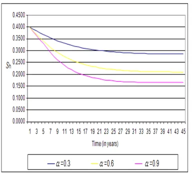
Figure 4.1.5. Graph showing the dynamics of the disease on the modified model with a vaccination rate of 0.3, 0.6 and 0.9 on the susceptible human population, corresponding to table 5 in the appendix.

4.2. Experiment One

Here the dynamics of the disease is compared between the old model and the modified. The experiment is carried out to establish the fact that a combination of both treat-ment and vaccination reduces the infectious population much more than applying treatment alone, as it was, in the result obtained from the old model.

4.3. Experiment Two

In this experiment, the dynamics of the disease of the modified model under the treatment and vaccination rate of 0.6 is carried out and compared with the old model of treatment rate of 0.6. We observed that a combination of the control measures causes a further decline in the infec-tious population from 0.24 to 0.008 through 0.0984 and 0.0101

4.4. Experiment Three

In this experiment, the dynamics of the disease of the modified model under the treatment and vaccination rate of 0.9 is carried out and compared with the old model with just treatment rate of 0.9. The result in this experiment shows that eradication is possible provided that both con-trol measure rates are maintained.

4.5. Experiment Four

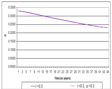
In this experiment, the dynamics of the disease on in-fected vector of the modified model under the treatment and vaccination rate of 0.3 is carried out and compared with the old model of treatment rate of 0.3. The infected vector populationdrops from 0.330 to 0.2330 and 0.2320. This will mean that less infectious vector population will be available for susceptible human to become infectious. Furthermore, the existence of mosquitoes will not necessar-ily increase the rate of malaria infection. There are many places in the world where mosquitoes abound but have not yet recorded malaria cases. Such places include Cape Town

in South Africa, Maryland in USA, Kyoto in Japan, etc.

4.6. Experiment Five

In this experiment, we examine the effect of increasing vaccination rate from 30% through to 90%, we observed that the susceptible human population drop from 0.4000 to 0.1654 through 0.2102. Since the susceptible human popu-lation will not much be available, it makes it difficult for infectious mosquitoes to cause infections on human popu-lation. This in the long run should result into a malaria-free society.

4.7. Discussion of Results

The result from experiment one shows that in the ab-sence of vaccination, eradication of the disease cannot be achieved so fast compared with combining vaccination along with treatment, as in the case in experiment two and three. The result for the infectious human population in experiment three carried out under a combined treatment and vaccination rate of 0.9 declines faster, thus resulting in a malaria-free society.

5. Summary, Conclusion, and

Recom-mendation

5.1. Summary

The Tumwiine et al. (2007) mathematical model for the dynamics of malaria within human host and mosquito vec-tors was modified by adding a vaccination parameter. The model was analyzed in terms of actual population. The stability of the equilibrium point obtained were analyzed and found to be locally asymptotically stable. The effect of vaccination on the susceptible human class of the modified SIR host and SI vector model was considered. It was ob-served that, gradually increasing the vaccination rate alone reduces the number of susceptible human population against possible re-infection, thus in the long run decrease the number of infectious human population gradually to a barest minimal level. Numerical experiments carried out on the modified model clearly shows that, with a proper com-bination of treatment and a concerted effort aimed at pre-vention, malaria can be eliminated.

5.2. Conclusion

(9)

Recommendations

In consideration of the findings of this study as well as the incidental observations, we recommend that a combina-tion of treatment and vaccinacombina-tion rates should be main-tained at 0.65 level in order to eradicate malaria in the pop-ulation.

Finally, it should be possible to validate this model by applying it to a smaller population, and then to a larger portion of any country. This will allow us to make in-formed decisions about the level of control strategies, “vaccination”, that provide the most effective way of eradi-cating malaria.

References

[1] Aslan G, Seyrek A. (2007). The diagnosis of malaria and identification of plasmodium species by polymerase chain reaction in turkey. pp:87-102

[2] Deressa, Wakgari, Ali, Ahmed and Berhane, (2000). Ye-mane Maternal responses to childhood febrile illnesses in an area of seasonal malaria transmission in rural ethiopia. Acta

tropica, pp: 134-166

[3] Dietz, Molineaux and Thomas (1974) Development of a new version of the Liverpool malaria model. Oxford Uni-versity Press, Oxford.

[4] Kakkilaya, B. S. (2003). Rapid diagnosis of malaria, lab medicine, 8(34), 602-608

[5] Nedelman J. (1985) Estimation for a model of multiple malaria infections. Phil. Trans. R. Soc. London. 65(4), 291: 451-524

[6] Perandin F. (2003). Development of a Real-time PCR assay for detection of plasmodium falciparum, plsmodium vivax, and plasmodium ovale for routine clinical diagnosis. Journal of clinical microbiology, 42 (3), 1214-1219, A Moody, Rap-id diagnostic tests for malaria parasites, Clin Microbiol Rev 15 (2002), pp. 66–78.

[7] Tumwiine, Mugisha J. Y. T and Lubobi L. S (2007). Applied mathematics and computation. 189(2007) pp1953-1965. [8] Yang Hyun. M, (2000) Mapping and predicting malaria