From Integral Representation Method (IRM) to Generalized Integral Representation Method (GIRM)

(1)

Published online February 10, 2015 (http://www.sciencepublishinggroup.com/j/acm) doi: 10.11648/j.acm.s.2015040301.11

ISSN: 2328-5605 (Print); ISSN: 2328-5613 (Online)

From Integral Representation Method (IRM) to Generalized

Integral Representation Method (GIRM)

Hiroshi Isshiki

IMA, Institute of Mathematical Analysis, Osaka, Japan

Email address:

[email protected]

To cite this article:

Hiroshi Isshiki. From Integral Representation Method (IRM) to Generalized Integral Representation Method (GIRM). Applied and Computational Mathematics. Special Issue: Integral Representation Method and its Generalization. Vol. 4, No. 3-1, 2015, pp. 1-14. doi: 10.11648/j.acm.s.2015040301.11

Abstract:

Integral Representation Method (IRM) is one of convenient methods to solve Initial and Boundary Value Problems (IBVP). It can be applied to irregular mesh, and the solution is stable and accurate. However, it was originally developed for linear equations with known fundamental solutions. In order to apply to general nonlinear equations, we must generalize the method. In the present paper, a generalization of IRM (GIRM) is discussed and applied to specific problems and the numerical solutions obtained. The numerical results are stable and accurate. The generalized method is called Generalized Integral Representation Method (GIRM). Brief explanations on the relationships with other numerical methods are also given.

Keywords:

Initial and Boundary Value Problems (IBVP), Integral Representation Method (IRM), Generalized Integral Representation Method (GIRM), Generalized Fundamental Solution

1. Introduction

Integral Representation Method is one of convenient methods to solve Initial and Boundary Value Problems (IBVP) [1-3]. It can be applied to irregular mesh, and the solution is stable and accurate. However, it was originally developed for linear equations with known fundamental solutions. In order to apply to general nonlinear equations, we must generalize the method [4-6]. In IRM, the fundamental solution satisfying a proper differential equation is sought based on our knowledge of the differential equation. However, in Generalized Integral Representation Method (GIRM), we assume the proper fundamental solution in advance. Choice of the fundamental solution may always be possible.

In the present paper, the generalization of IRM is discussed not only from the theoretical viewpoint, but also the computational aspects are also discussed. GIRM is applied diffusion problems and Burgers’ equation. The numerical results are stable and accurate.

In the present paper, IRM and GIRM are explained from very basic level to advanced level, and the relationships with other numerical methods such as Finite Difference Method (FDM) and Collocation Method (CM) etc. are also clarified.

2. Preparation

As a basis of discussion, we discuss the solution of one-dimensional Initial Boundary Value Problem (IBVP) of one-dimensional diffusion problem in flow.

Let x and t refer to the coordinate and time, respectively. IBVP of one-dimensional diffusion in flow is given by

σ

κ +

∂ ∂ = ∂ ∂ + ∂ ∂

2 2

x C x

C U t C

in −L<x<L & t>0, (1)

) (t g

C= −L at x=−L & t>0

and C=gL(t) at x=L & t>0, (2)

) (x f

C= in −L<x<L at t=0, (3)

where C(x,t), U , σ(x,t) and κ are the density of substance, velocity of flow, source of substance and constant of diffusion, respectively. The functions g_λ(t) (λ=−L,L) and f(x) give the boundary and initial values of the density C(x,t), respectively.

A numerical solution of IBVP can be obtained by the following procedure:

) , (xt

(2)

Eq. (1)

→

obtain C(x,t+dt) from

t t x C dt t x C dt x

C( + )= ( , )+ ⋅∂ ( , ) ∂

→

add dt to t

→

repeat. (4)

2.1. Finite Difference Method (FDM)

In Finite Difference Method (FDM), the differential equation Eq. (1) is discretized directly using Differences.

We adopt a regular mesh or grid:

N L

dx=2 , xi=−L+idx i=0,1,⋯,N, (5)

ndt

tn = n=0,1,⋯, (6)

) , (

) (

n i n

i C x t

C = , ( ) ( , )

n i n

i σ x t

σ = . (7)

The space derivatives are approximated using central differences:

(

( , ) ( , )

)

2 1

t dx x C t dx x C dx x

C ₌ ₊ ₋ ₋

∂ ∂

. (8a)

(

( , ) 2 ( , ) ( , )

)

1

2 2 2

t dx x C t x C t dx x C dx x

C

− + −

+ =

∂ ∂

. (8b)

Then, we obtain an approximation of IBVP defined by Eqs. (1-3):

(

)

(

( )

)

( )

1 ) ( ) (

1 2 ) (

1 ) (

1 )

(

2 2

n i n i n i n i n

i n i n

i

C C C dx C C dx U t

C ₌₋ ₋ ₊ κ ₋ ₊ ₊_σ

     

∂ ∂

− +

for i=1,⋯,N−1 & n=1,⋯, (9)

) (

0 L n

n

t g

C = ₋ , ( ) L(n)

n N g t

C = for n=0,1,⋯, (10)

) (

) 0 (

i i f x

C = for i=1,⋯,N−1, (11)

where () ( i, n)

n

i C x t

C = , etc.

If we use Explicit Time Evolution (ETE),

[

∂C ∂t

]

(in) is

interpreted as

(

( 1) ( )

)

) (

1 n

i n i n

i

C C dt t

C

− =

     

∂

∂ +

or dt

t C C

C

n

i n

i n i

) ( )

( ) 1 (

     

∂ ∂ + = +

. (12)

) 1 (n+ i

C is obtained by the following procedure:

) (n i

C is known at t

→

obtain

[

∂C ∂t

]

(in) from

Eq. (9)

→

obtain (n+1)

i

C from

[

∂C ∂t

]

(_in)

using Eq. (12)

→

add

dt

to t

→

repeat. (13)

If we use Implicit Time Evolution (ITE),

[

∂C ∂t

]

(in) is

understood as

(

( ) ( 1)

)

) (

1 ₋ −

=

     

∂

∂ n

i n i n

i

C C dt t

C

, (14)

and we substitute Eq. (14) into Eq. (9):

(

( ) ( 1)

)

1 ₋ n−

i n

i C

C dt

(

)

(

()

)

()

1 ) ( ) (

1 2 ) (

1 ) (

1 2

2

n i n i n i n i n

i n

i C C C

dx C C dx

U ₋ ₊ κ ₋ ₊ ₊_σ

−

= + − + −

for i=1,⋯,N−1 & n=1,⋯, (15)

) (n i

C is obtained by the following procedure:

) 1 (n− i

C is known at t

→

obtain (n)

i

C solving

an algebraic equation Eq. (15)

→

add dt to

t

→

repeat. (16)

FDM-ITE requires inversion of matrix.

FDM discretizes the differential equation into difference equation. FDM is accurate if we use highly accurate difference such as central difference, but FDM requires regular grid. FDM-ETE does not require inversion of matrix. This is very helpful to reduce computational time.

2.2. Mode Function Interpolation Method (MFIM)

The unknown function C(x,t) could be interpolated before obtaining discretizing the equations. We may call this method Mode Function Interpolation Method (MFIM). Collocation Method (CM), Conventional Galerkin Method (CGM) and Finite Element Method (FEM) etc., belong to MFIM. CM and CGM apply MFIM in global region, and FEM does in local regions.

In case of CM, we use MFIM of the following form:

∑

− =

= 1

0

) ( ) ( )

, (

M

x G t c t x C

µ µ µ

in −L≤x≤L & t≥0, (17)

where Gµ(x) is a mode function. cµ(t) is the coefficient of interpolation and corresponds to generalized coordinates in analytical mechanics.

If we substitute Eq. (17) into Eq. (1-3), we obtain

σ κ

µ

µ µ

µ

µ µ

µ

+ +

−

=

∑

−

= −

=

1

0

2 2 1

0 1

0

) ( ) ( )

( ) (

) ( ) (

M M

M

dx x G d t c dx

x dG t c U

x G dt

t dc

(3)

) ( ) ( ) ( 1

0

t g L G t

c L

M

− −

= − =

∑

µ µ µ

at t>0

and () ( ) ()

1

0

t g L G t

c L

M

=

∑

− =

µ µ µ

at t>0, (19)

) ( ) ( ) 0 ( 1

0

x f x G c

M

=

∑

− =

µ µ µ

in −L<x<L. (20)

We can use a irregular mesh or grid in CM:

L x x x x

L, 1, 2, , N−2, N−1,

− ⋯ , (21)

ndt

tn = n=0,1,⋯, (22)

) ( ) (

n n

t c

cµ = µ , ( ) ( i, n) n

i σ x t

σ = . (23)

The discretized equations of IBVP using CM are given by

) (

0

2 2 ) (

0 ) ( 0

) (

) ( )

( ) (

n i M

i n

M

i n

M

i n

dx x G d c dx

x dG c U

x G dt dc

σ κ

µ

µ µ µ

µ µ

µ µ µ

+ +

− =

     

∑

= =

=

for i=1,2,⋯,N−1 & n=1,2,⋯, (24)

) ( ) ( 0

) (

n L M

n

t g L G

c ₋

=

= −

∑

µ µ µ

, ( ) ( )

0 ) (

n L M

n

t g L G

c =

∑

=

µ µ µ

for n=1,⋯, (25)

) ( ) ( 0

) 0 (

i M

i f x

x G

c =

∑

=

µ µ µ

for i=1,2,⋯,N−1. (26)

If we use Implicit Time Evolution (ITE),

[

dc dt

]

(_µn) is understood as

(

( ) ( 1)

)

) (

1 ₋

− =

    

 n n

n

c c dt dt

dc

µ µ µ

, (27)

we substitute Eq. (14) into Eq. (24):

(

)

) (

0

2 2 ) (

0 ) ( 0

) 1 ( ) (

) ( )

( ) ( 1

n i M

i n

M

i n

M

i n

n

dx x G d c dx

x dG c U

x G c c dt

σ κ

µ

µ µ µ

µ µ

µ µ µ µ

+ +

− =

−

∑

= =

=

−

for i=1,⋯,N−1 & n=1,⋯, (28)

) (n

c_µ is obtained by the following procedure:

) 1 (n−

c_µ is known at t−1

→

obtain (n) c_µ from

Eqs. (28) and (25)

→

add dt to t

→

repeat. (29)

If N and M satisfy

M

N+1≥ , (30)

we can apply Least Square Method (LSM) to determine )

(n

c_µ (µ=0,1,⋯,M−1).

CM does not require regular mesh. If proper mode functions are used, the accuracy is high.

If g−L(t)and gL(t) satisfy

0 )

( =

− t

g L , gL(t)=0, (31)

we can make mode function G_µ(x) satisfy

0 ) ( )

(−L =G L =

Gµ µ for µ=0,1,⋯,M −1. (32)

Then, Eqs. (24-26) are replaced by

) (

0

2 2 ) (

0 ) ( 0

) (

) ( )

( ) (

n i M

i n

M

i n M

i n

dx x G d c dx

x dG c U

x G dt dc

σ κ

µ

µ µ µ

µ µ

µ µ µ

+ +

− =

     

∑

= =

=

for i=1,2,⋯,N−1 & n=1,⋯ (33)

) ( ) ( 0

) 0 (

i M

i f x

x G

c =

∑

=

µ µ µ

for i=1,2,⋯,N−1. (34)

In this case, we can also apply ETE.

[

dc dt

]

(_µn) is interpreted as

(

( 1) ( )

)

) (

1 n n

n

c c dt dt

dc

µ µ µ

− =

    

 ₊

or dt

dt dc c c

n n

n

) ( ) ( ) 1 (

µ µ

µ+ = +_ _ . (35)

) 1 (n+

cµ is obtained by the following procedure:

) (n

cµ is known at t

→

obtain

[

dc dt

]

(µn) from

Eq. (33)

→

obtain (n+1)

c_µ from

[

dc dt

]

(_µn)

using Eq. (35)

→

add dt to t

→

repeat. (36)

3. Integral Representation Method (IRM)

Eq. (17) suggests us an integral representation of dependent variable:

ξ ξ

ξ c t d

x G t x

C( , ) L ( , ) ( , )

0

∫

=

in −L≤x≤L & t≥0. (37)

(4)

∫

∑

= = = = = = = L M M M d t c x G d d x G t d c d x G t c L M x G t c t x C 0 0 0 0 ) , ( ) , ( ) , ( ) , ( ) ( ) ( 2 ) ( ) ( ) , ( ξ ξ ξ ξ ξ µ ξ µ ξ µ

µ µ µ

, (38)

where

M L

dξ =2 , cµ(t)=c(µdξ,t), ( , ) 2

)

( µ ξ

µ G x d

L M x

G = . (39)

Multiplying a function G(x,ξ) of x and ξ on both side of Eq. (1)

∫

₋           − ∂ ∂ − ∂ ∂ + ∂ ∂ = L

L G x dx

t x x t x C x t x C U t t x C ) , ( ) , ( ) , ( ) , ( ) , ( 0 2 2 ξ σ κ

∫

₋                     − ∂ ∂       ∂ ∂ + − +       ∂ ∂ − ∂ ∂ + ∂ ∂ = L L dx x G t x x x G x t x C t x UC x G x t x C x G t x UC x x G t t x C ) , ( ) , ( ) , ( ) , ( ) , ( ) , ( ) , ( ) , ( ) , ( ) , ( ) , ( ξ σ ξ κ ξ κ ξ ξ

∫

₋                     ∂ ∂ −       ∂ ∂ ∂ ∂ + ∂ ∂ − ∂ ∂ = L L dx x x G t x C x x G t x C x x x G x UC x G t t x C 2 2 ) , ( ) , ( ) , ( ) , ( ) , ( ) , ( ) , ( ) , ( ξ κ ξ κ ξ ξ ξ

∫

₋ = − = −       ∂ ∂ − + L L L x L x dx x G t x x G x t x C x G t x UC ) , ( ) , ( ) , ( ) , ( ) , ( ) , ( ξ σ ξ κ ξ

∫

− − − ∂ ∂ − ∂ ∂ − ∂ ∂ = L L L L L L dx x x G t x C dx x x G t x C U dx x G t t x C 2 2 ) , ( ) , ( ) , ( ) , ( ) , ( ) , ( ξ κ ξ ξ

[

]

L x L x L x L x x x G t x C x G x t x C x G t x C U = − = = − =       ∂ ∂ − ∂ ∂ − + ) , ( ) , ( ) , ( ) , ( ) , ( ) , ( ξ ξ κ ξ

∫

₋ − L

Lσ(x,t)G(x,ξ)dx. (40)

Rewriting Eq. (40), we have

∫

− − − ∂ ∂ + ∂ ∂ = ∂ ∂ L L L L L L dx x x G t x C dx x x G t x C U dx x G t t x C 2 2 ) , ( ) , ( ) , ( ) , ( ) , ( ) , ( ξ κ ξ ξ

[

]

L x L x L x L x x x G t x C x G x t x C x G t x C U = − = = − =       ∂ ∂ − ∂ ∂ + − ) , ( ) , ( ) , ( ) , ( ) , ( ) , ( ξ ξ κ ξ .

∫

₋ + L

Lσ(x,t)G(x,ξ)dx (41)

Exchanging x and ξ, we obtain

∫

− − − ∂ ∂ + ∂ ∂ = ∂ ∂ L L L L L L d x G t C d x G t C U d x G t t C ξ ξ ξ ξ κ ξ ξ ξ ξ ξ ξ ξ 2 2 ) , ( ) , ( ) , ( ) , ( ) , ( ) , (

[

]

L L L L x G t C x G t C x G t C U = − = = − =       ∂ ∂ − ∂ ∂ + − ξ ξ ξ ξ ξ ξ ξ ξ ξ ξ κ ξ ξ ) , ( ) , ( ) , ( ) , ( ) , ( ) , ( .

∫

₋ + L

Lσ(ξ,t)G(ξ,x)dξ (42)

If G(x,ξ) is a fundamental solution of the differential

operator 2 2

x

∂

∂ , G(x,ξ) is defined as

) ( ) , ( 2 2 ξ δ

ξ ₌ ₋

∂ ∂ x x x G

, (43)

where δ(x) is Dirac’s delta function:

1 )

( =

∫

₋∞_∞δ x dx and δ(x)=0 when x≠0. (44)

Specifically, G(x,ξ):

| | 5 . 0 ) , ( ) ,

(xξ =Gξ x = x−ξ

G (45)

is a fundamental solution of the differential operator 2 2

x

∂

∂ .

Substituting Eq. (43) into Eq. (42) becomes

∫

− − − − ∂ ∂ − ∂ ∂ = L L L L L L d x G t d x G t C U d x G t t C t x C x ξ ξ ξ σ ξ ξ ξ ξ ξ ξ ξ κε ) , ( ) , ( ) , ( ) , ( ) , ( ) , ( ) , ( ) (

[

]

L

x G t C

U =₌₋

+ ξ

ξ

ξ ξ, ) ( , )

( , L L x G t C x G t C = − =       ∂ ∂ − ∂ ∂ − ξ ξ ξ ξ ξ ξ ξξ

κ ( , ) ( , ) ( , ) ( , ) (46)

(5)

     − = < < − = otherwise 0 , when 5 . 0 when 1 )

( x L L

L x L x

ε . (47)

Eq. (42) or (46) is an integral representation of Eq. (1). (1) Steady solution

If there exists a steady solution:

) ( ) , (

limC xt C x

t→∞ = , tlim→∞σ(x,t)=σ(x),

L L

t→∞g− (t)=g−

lim , L L

t→∞g (t)=g

lim (48)

we have from Eq. (46)

∫

₋ − ₋ ∂ ∂ − = L L L

L d G x d

x G C U x C x ξ ξ ξ σ ξ ξ ξ ξ κε ) , ( ) ( ) , ( ) ( ) ( ) (

[

]

L L L L x G C x G d dC x G C U = − = = − =       ∂ ∂ − − + ξ ξ ξ ξ ξ ξ ξ ξ ξξ κ ξ ξ ) , ( ) ( ) , ( ) ( ) , ( ) (

. (49)

If we substitute boundary condition into Eq. (46) and set x to −L and L, we obtain

∫

₋ ₋ − =− ∂ _∂ − − − L L L L

L d G L d

L G C U

g ξ σ ξ ξ ξ

ξ ξ ξ

κ ( ) ( , ) ( ) ( , )

2 1

[

g G(L, L) g G( L, L)

]

U L − − L − −

+ −

[

C′(L)G(L,−L)−C′(−L)G(−L,−L)

]

−κ ,

[

gLG (L,−L)−g LG (−L,−L)

]

+κ ξ − ξ , (50)

∫

₋ − ₋ ∂ ∂ − = L L L L

L d G L d

L G C U

g ξ σ ξ ξ ξ

ξ ξ ξ

κ ( ) ( , ) ( ) ( , )

2 1

[

g G(L,L) g G( L,L)

]

U L − L −

+ −

[

C′(L)G(L,L)−C′(−L)G(−L,L)

]

−κ

[

gLG (L,L)−g LG (−L,L)

]

+κ ξ − ξ , (51)

respectively. Eqs. (49), (50) and (51) are algebraic equations with unknowns C(x) in −L<x<L, C′(−L) and C′(L). If we have U=0, then, Eqs. (50) and (51) are algebraic equations with unknowns C′(−L) and C′(L).Hence, we can determine C′(−L) and C′(L) solving Eqs. (50) and (51). This is the one-dimensional case of Boundary Element Method (BEM). Substituting C′(−L) and C′(L) into Eq. (49), we can obtain C(x) in −L<x<L.

(2) Unsteady solution

If we know C(x,t) in −L≤x≤L, Eq. (46) is an integral equation with unknowns ∂C(x,t) ∂t in −L<x<L ,

) , ( L t

Cx − and Cx(L,t), where G(x,ξ) is the kernel function

of the integral equation.

We introduce, for example, a regular mesh:

N L d

dx= ξ =2 , xi =ξi =−L+(i+0.5)dx

1 , , 1 , 0 − = N

i ⋯ , (52)

ndt

tn = n=0,1,⋯, (53)

) , ( ) ( n i n

i C x t

C = , ( ) ( i,n)

n

i σ x t

σ = , (54a)

t t C t

C j n

n j ∂ ∂ =       ∂

∂ ( ) (ξ , )

. (54b)

We prepare for discretization of Eq. (46)

∑

∫

∑∫

∫

− = + − − = + − −       ∂ ∂ = ∂ ∂ = ∂ ∂ 1 0 2 2 ) ( 1 0 2 2 ) , ( ) , ( ) , ( ) , ( ) , ( N j d j d j n j N j d j d j n L L n d x G t C d x G t t C d x G t t C ξ ξ ξ ξ ξ ξ ξ ξ ξ ξ ξ ξ ξ ξ ξ ξ

, (55a)

) , ( ) , ( ) , ( ) , ( ) , ( ) , ( L x G t L C L x G t L C x G t C n n L L n − ∂ − ∂ − ∂ ∂ =       ∂ ∂ = − = ξ ξ ξ ξ ξ ξ

ξ _{, (55b)}

∑

∫

∑∫

∫

− = + − − = + − − = = 1 0 2 2 ) ( 1 0 2 2 ) , ( ) , ( ) , ( ) , ( ) , ( N j d j d j n j N j d j d j n L L n d x G d x G t d x G t ξ ξ ξ ξ ξ ξ ξ ξ ξ ξ σ ξ ξ ξ σ ξ ξ ξ σ

, (55c)

ξ ξ ξξ ξ ξ ξ ∂ − ∂ − ∂ ∂ =       ∂ ∂ − = − = ) , ( ) ( ) , ( ) ( ) , ( ) , ( L x G t g L x G t g x G t C n L n L L L n

, (55d)

where ∂C(ξj,tn) ∂t=Cξ(ξj,tn) etc. Eq. (46) can be discretized as

      − ∂ − ∂ − ∂ ∂ − Γ       ∂ ∂

∑

− = ) , ( ) , ( ) , ( ) , ( ) ( 1 0 ) ( x L G t L C x L G t L C x t C n n N j j n j ξ ξ κ

∑

− = −

= Λ + Γ

+ = 1 0 ) ( 1 0 ) ( ) ( ) ( ) , ( ) ( N j j n j N j j n j

n U C x x

t x C

x σ

(6)

[

g (t )G(L,x) g (t )G( L,x)

]

U L n − L n −

− −

   

 

∂ − ∂ −

∂ ∂

−κ gL(tn) G(L_ξ,x) g−L(tn) G(_ξL,x) , (56)

where

∫

₋+ =

Γ 2

2 ( , )

)

( ξ ξ

ξ

ξ ξ ξ

d j

j x G x d ,

∫

+

− _∂

∂ =

Λ 2

2

) , ( )

( ξ ξ

ξ

ξ ξ ξ

ξ

d j

j d

x G

x . (57)

The unknowns are

[

∂C ∂t

]

(jn) ( j=0,1,⋯,N−1 ),

ξ

∂ −

∂C( L,tn) and ∂C(L,tn) ∂ξ. Eq. (56) is satisfied at the

center points x=x0,x1,⋯,xN−1 of elements and boundary points x=0,L. Hence, we have N+2 equations for N+2

unknowns.

If we approximate ∂C(−L,tn) ∂ξ and ∂C(L,tn) ∂ξ by

(

( , ) ( , )

)

2 ) , (

0 n n

n

t L C t x C d t L C

− − =

∂ − ∂

ξ

ξ , (58a)

(

( , ) ( , )

)

2 ) , (

1 n N n

n

t x C t L C d t L C

−

− + =

∂ + ∂

ξ

ξ (58b)

and satisfy Eq. (56) at the center points x=x0,x1,⋯,xN−1 of elements, then we have N equations for

N

unknowns.

Although IRM is mathematically complex and requires matrix inversion, but the accuracy of the numerical result is high. It can be applied to irregular mesh. If the computer code is properly written, the computational load may be comparable with Finite element Method (FEM).

4. Generalized Integral Representation

Method (GIRM)

IRM is basically developed for a linear problem with a known fundamental solution for the differential equation. Hence, if we have an IBVP using a differential equation different from Eq. (1), for example:

σ

κ +

∂ ∂ = ∂ ∂

4 4

x C t

C

in −L<x<L & t>0, (59)

we must find first a fundamental solution satisfying

) ( ) , (

4 4

ξ δ

ξ ₌ ₋

∂ ∂

x x

x G

(60)

In order to apply IRM to any kinds of linear and nonlinear problems, we must generalize the method. For the purpose, we generalize the concept of the fundamental solution. We replace Eq. (43) by

) , ( ~ ) , ( ~

2 2

ξ δ ξ

x x

x G

= ∂ ∂

, (61)

where δ~(x,ξ) can be

) ( ) , ( ~

ξ δ ξ

δ x ≠ x− . (62)

) , (

~ _ξ

x

G is a generalized fundamental solution chosen properly, for example

   

  ₋

−

= 2

2

2 ) ( exp 2

1 ) , ( ~

γξ γ

π

ξ x

x

G (63)

The function δ~(x,ξ) is not Dirac’s delta function as in Eq. (43), but it is nothing but the second derivatives of G~(x,ξ)

with respect to x.

Multiplying G~(x,ξ) on both side of Eq. (1), we obtain similar to Eq. (41):

∫

−

− −

∂ ∂ +

∂ ∂ =

∂ ∂

L L

L L L

L

dx x

x G t x C

dx x x G t x C U dx x G t

t x C

2 2

) , ( ~ ) , (

) , ( ~ ) , ( )

, ( ~ ) , (

ξ κ

ξ ξ

[

]

L x

L x L

x L x

x x G t x C x G x

t x C

x G t x C U

=

− = =

− =

   

   

∂ ∂ −

∂ ∂ + −

) , ( ~ ) , ( ) , ( ~ ) , (

) , ( ~ ) , (

ξ ξ

κ

ξ

∫

₋

+ L

L xtG(x, )dx

~ ) ,

( ξ

σ . (64)

Exchanging x and ξ, we obtain

∫

−

− −

∂ ∂ +

∂ ∂ =

∂ ∂

L L

L L L

L

d x G t C

d x G t C U d x G t

t C

ξ ξξ ξ

κ

ξ ξ ξ ξ ξ

ξ ξ

2 2

) , ( ~ ) , (

) , ( ~ ) , ( )

, ( ~ ) , (

[

]

L

x G t C

U =₌₋

− (ξ, )~(ξ, )ξξ

L

L x G t C x G t

C =

− =

    

  

∂ ∂ − ∂

∂ +

ξ

ξ ξ ξ ξ

ξ ξ

κ ( , )~( , ) ( , ) ~( , )

∫

₋

+ L

Lσ ξ tG(ξ,x)dξ

~ ) ,

( . (65) This is a generalized integral representation of Eq. (1). This integral representation is applied to numerical solution of IBVP in the similar way as discussed for IRM. This numerical method is called GIRM.

Numerical examples are given below. The initial condition is doublet-like and given by

dx x d x

x x

x

C( ,0) ( ) ( ) ( )

0 0

δ ξ

δ ξ ξ

δ

ξ ξ

− = ∂

− ∂ − = ∂

− ∂ =

(7)

or

     

= +

− = −

=

otherwise 0

2 for

1

1 2 for

1

2 2

) 0 (

N i dx

Ci . (66)

We assume that L is big enough, and the boundary condition is specified as

0 ) , ( ) ,

(±Lt =C ±Lt =

C x . (67)

The exact solution is given by

t Ut x t Ut x t

t Ut x t

x t x C

ν ν

πν

ν πν

2 4

) ( exp 2

1

4 ) ( exp 2

1 )

, (

2

−

   

  ₋

− =

   

   

   

  ₋

− ∂

∂ − =

. (68)

The parameters for numerical calculations are as follows:

4 =

L ; N=160; dx=2L 8=0.05; γ =0.75dx;

0005 . 0

=

dt ; T =3000dt; κ=0.089; U =0,1. (69)

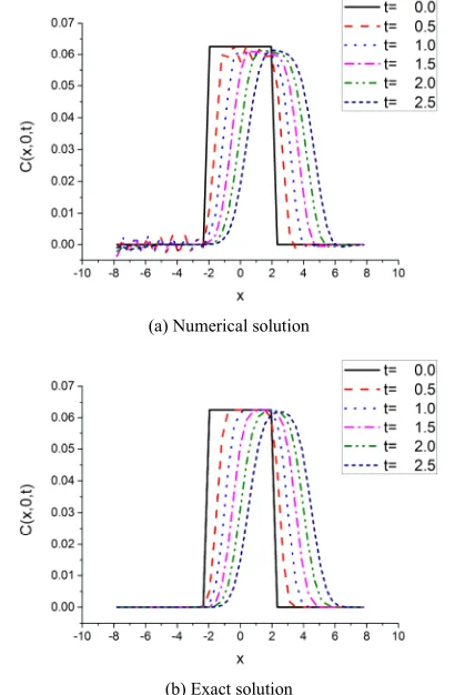
Numerical results are shown Figs. 1 and 2. Because of the singular initial condition, we need very fine mesh. The accuracy of the numerical results is very high. The numerical results coincide with the exact ones.

5. Further Generalization of General

Integral Representation Method

(GIRM)

A further generalization of GIRM in one-dimensional case is discussed below:

) , ( ,

, , , ,

, ₂

2

t x f x

u x

u x u u t x F t u

N N

=

   

 

∂ ∂ ∂ ∂ ∂ ∂ +

∂ ∂

⋯

in −L<x<L & t>0. (70)

x u

∂ ∂ =

1

θ ,

x

∂ ∂ = 1 2

θ

θ , … ,

x

N N

∂ ∂ = θ −1

θ , (71)

(

x,t,u, 1, 2, ,

)

f(x,t) F

t u

N =

+ ∂

∂ _θ _θ _θ

⋯ . (72)

We introduce a generalized fundamental solution G~(x,ξ)

and the derivative δ~1(x,ξ) with respect to x, for example

   

  ₋

−

= 2

2

2 ) ( exp 2

1 ) , ( ~

γξ γ

π

ξ x

x

G , (73a)

) , ( ~ ) , ( ~

1 ξ

δ ξ

x x

x

G ₌

∂ ∂

. (73b)

We use the following formula:

x x G t x x

x G t x

x G x

t x

n n

n

∂ ∂ −

∂ ∂ =

∂ ∂

− −

−

) , ( ~ ) . ( ) , ( ~ ) . (

) , ( ~ ) . (

1 1

1

ξ θ

. (74)

Applying Eq. (74) to each of Eq. (71), we have

∫

₋ −

   

 

∂ ∂ − = L

L

n

n G x dx

x t x t

x, ) ( , ) ~( , )

(

0 θ θ 1 ξ

∫

₋ −

−

   

 

   

 

∂ ∂ +

∂ ∂ − = L

L n

n n

dx

x x G t x

x x G t x t

x x G

) , ( ~ ) , (

) , ( ~ ) , ( )

, ( ) , ( ~

1

ξ θ

θ ξ

[

]

x L

L x n

L

LG x n xt dx xt G x

= − = −

− −

=

_∫

~( ,ξ)θ ( , ) θ 1( , )~( ,ξ) .

∫

₋ −

+ L

L n xt (x, )dx

~ ) ,

( 1

1 δ ξ

θ (75)

Rewriting Eq. (75), we obtain

[

]

x L

L x n

L L n L

L n

x G t x

dx x t x dx

t x x G

= − = −

− −

−

+

− =

∫

) , ( ~ ) , (

) , ( ~ ) , ( )

, ( ) , ( ~

1

1 1

ξ θ

ξ δ θ θ

ξ

. (76)

Exchanging x and ξ , we obtain a generalized integral representation:

[

]

L

L n

L L n L

L n

x G t

d x t d

t x G

= − = −

− −

−

+

− =

_∫

∫

ξ ξ

ξ ξ θ

ξ ξ δ ξ θ ξ ξ θ ξ

) , ( ~ ) , (

) , ( ~ ) , ( )

, ( ) , ( ~

1

1 1

. (77)

Eq. (74) is the integral representation of Eq. (71).

The integral representation of Eq. (72) is obtained below. Multiplying G~(x,ξ) on both sides of Eq. (72) and integrating

in G~(x,ξ) with respect to t, we have

(8)

(b) Exact solution

Figure 1. Doublet-like initial density distribution (U=0).

(a) Numerical solution

(b) Exact solution

Figure 2. Doublet-like initial density distribution (U=1).

∫

₋ ∂ _∂

= L

L _t dx

t x u x

G~( , ) ( , )

0 ξ

(

)

∫

₋

+ L

LF xt u xt xt xt N xt G(x, )dx

~ ) , ( , ), , ( ), , ( ), , ( ,

, θ1 θ2 ⋯θ ξ

∫

₋

− L

Lf xt G(x, )dx

~ ) ,

( ξ . (78)

Exchanging x and ξ, we obtain a generalized integral representation for Eq. (72):

∫

₋ ∂ _∂

= L

L _t d

t u x

G~(ξ, ) (ξ, ) ξ 0

(

)

∫

₋

+ L

LFξ t uξ t θ ξ t θ ξ t θN ξ t G(ξ,x)dξ

~ ) , ( , ), , ( ), , ( ), , ( ,

, ₁ ₂ _⋯

∫

₋

− L

Lf ξ t G(ξ,x)dξ

~ ) ,

( . (79)

) , (xt

u is obtained by the following procedure:

) , (xt

u is known

→

θ1(x,t) from Eq. (77)

→

θ2(x,t) from Eq. (77)

→

…

→

θn−1(x,t)

from Eq. (77)

→

∂u(x,t) ∂t from Eq. (79)

→

) , (xt dt

u + from ∂u(x,t) ∂t

→

repeat. (80)

6. Generalized Integral Representation

Method (GIRM) in Multi-Dimensional

Space

6.1. Application of GIRM to Diffusion in Flow

As a basis of discussion, we discuss the solution of Initial Boundary Value Problem (IBVP) of Nd -dimensional

diffusion in a flow.

If x_i , (i=1,2,⋯,Nd) and t refer to the coordinates and time, the diffusion equation in N_d -dimension is expressed as

σ

κ +

∂ ∂

∂ = ∂ ∂ + ∂ ∂

j j i i

x x

C x

C U t

C 2

. (81)

The summation convention is used for the repeated indices, that is,

d N d N i

i C x U C x U C x

U ∂ ∂ = 1∂ ∂ 1+⋯+ ∂ ∂ and

2 2 2

1 2 2

d N i

i x x x

x∂ =∂ ∂ + +∂ ∂

∂

∂ ⋯ . C, Ui and κ refer to

the density of substance, velocity vector of a given flow and diffusion constant, respectively. Since it’s not difficult to obtain two-dimensional expressions from three-dimensional ones, we develop theory using three-dimensional expressions below.

We rewrite the basic equation Eq. (81) as follows: Non-uniformity equation:

i i

x C

∂ ∂ =

θ . (82)

Constitutive equation:

i i

q =−κθ . (83)

Equilibrium equation:

i i i i

x q x C U t C

∂ ∂ − = ∂ ∂ + ∂ ∂

. (84)

(9)

solution G~(x,ξ) with scale γi , (i=1,2,⋯,Nd) [4,5], for example:

∏

=      ₋ − = Nd

i i i i i x G 1 2 2 2 ) ( exp 2 1 ) , ( ~ γξ γ π ξ

x , (85)

We obtain an integral representation of Eq. (82). From Eq. (85), we have

) , ( ~ ) , ( ) , ( ~ ) , ( ) , ( ~ ) , ( ξ x x ξ x x ξ x x j i i t C x G t C G x t

C ₋ _δ

∂ ∂ = ∂

∂

, (86)

where ) , ( ) , ( ~ ξ x ξ x i i x

G ₌_δ

∂ ∂

. (87)

Multiplying G~(x,ξ) on the both sides of Eq. (82) and integrating in region V , we obtain

∫∫∫

      ∂ ∂ − = V i

i G dV

x t C

t xξ x

x

x, ) ( , ) ~( , )

( 0 θ

∫∫∫

          + ∂ ∂ − = V i i i dV t C x G t C t G x ξ x x ξ x x x ξ x ) , ( ~ ) , ( ) , ( ~ ) , ( ) , ( ) , ( ~ δ θ

[

]

∫∫∫

+ =

V G xξ i xt C xt i(x,ξ)dVx

~ ) , ( ) , ( ) , (

~ _θ _δ

.

∫∫

− _SC xtG(x,ξ)nxidSx

~ ) ,

( . (88) Rewriting Eq. (88), we have

∫∫∫

=−

V i

VG xξ i xt dVx C xt (x,ξ)dVx

~ ) , ( ) , ( ) , (

~ _θ _δ

∫∫

+

SC xt G(x,ξ)nxidSx

~ ) ,

( . (89)

Exchanging x and ξ in Eq. (89), we obtain a generalized integral representation for Eq. (82):

∫∫∫

=−

V i

VG ξx i ξt dVξ C ξt (ξ,x)dVξ

~ ) , ( ) , ( ) , (

~ _θ _δ

∫∫

+

SG(ξ,x)C(ξ,t)nξidSξ

~

. (90)

A generalized integral representation of Eq. (84) is obtained similarly. From Eq. (87), we have

i i i i x G t C t U G x t C t U ∂ ∂ =       ∂ ∂ ( , ) ( , )~( , ) ) , ( ~ ) , ( ) ,

(x x xξ x x xξ

) , ( ~ ) , ( ) , ( ) , ( ~ ) , ( ) , ( ξ x x x ξ x x x i i i i t C t U G t C x t U _δ − ∂ ∂

− . (91a)

) , ( ~ ) , ( ) , ( ~ ) , ( ) , ( ~ ) , ( ξ x x ξ x x ξ x x i i i i i i t q x G t q G x t

q ₋ _δ

∂ ∂ = ∂ ∂ . (91b)

∫∫∫

      ∂ ∂ + ∂ ∂ + ∂ ∂ = V i i i i dV x t q x t C t U t t C G x x x x x ξ

x, ) ( , ) ( , ) ( , ) ( ,) ( ~ 0

∫∫∫

+ ∂ _∂ ∂ ∂ = V i i

V _x dV

G t C t U dV t t C

G xξ x _x x x (x,ξ) _x

~ ) , ( ) , ( ) , ( ) , ( ~

∫∫∫

      + ∂ ∂ −

V i i

i

i _C _t _G _U _t _C _t _dV

x t U x ξ x x x ξ x x x ) , ( ~ ) , ( ) , ( ) , ( ~ ) , ( ) , ( δ

∫∫∫

_       − ∂ ∂ +

V i i

i

i _q _t _dV

x t q G x ξ x x x ξ x ) , ( ~ ) , ( ) , ( ) , ( ~ δ

∫∫

∫∫∫

+ ∂ ∂ =

S i i

V _t dV G U t C t n dS

t C

G x x ξ x x x x

x ξ

x, ) ( , ) ~( , ) ( , ) ( , )

( ~

∫∫∫

      + ∂ ∂ −

V i i

i

i _C _t _G _U _t _C _t _dV

x t U x ξ x x x ξ x x x ) , ( ~ ) , ( ) , ( ) , ( ~ ) , ( ) , ( δ

∫∫∫

∫∫

− +

V i i

SG xξ qi x t nxidSx q x t (x,ξ)dVx

~ ) , ( ) , ( ) , ( ~

δ . (92)

∫∫∫

_V ∂ _∂ dV

t t C G x x ξ

x, ) ( , )

( ~

[

]

∫∫∫

+

=

V Ui xt C x t qi x t i(x,ξ)dVx

~ ) , ( ) , ( ) , ( δ

∫∫∫

∂ _∂ + V i

i _C _t _G _dV

x t U x ξ x x x ) , ( ~ ) , ( ) , (

[

]

∫∫

+ −

SG(x,ξ)Ui(x,t)C(x,t) qi(x,t)nxidSx

~

. (93)

Exchanging x and ξ in Eq. (93), we obtain a generalized integral representation of Eq. (84):

∫∫∫

V ∂ _∂_t dV

t C

G ξ

ξ x

ξ, ) ( , )

( ~

[

]

∫∫∫

+

=

V Ui ξt C ξ t qi ξt i(ξ,x)dVξ

~ ) , ( ) , ( ) , ( δ

∫∫∫

∂ _∂ + V i

i t _C _t _G _dV

U ξ x ξ ξ ξ ) , ( ~ ) , ( ) , ( ξ

[

]

∫∫

+ −

SG(ξ,x)Ui(ξ,t)C(ξ,t) qi(ξ,t)nξidSξ

~

. (94)

(10)

) , ( t

C x is known

→

θi(x,t) from Eq. (90)

→

) , ( t

qi x from Eq. (83)

→

∂C(x,t) ∂t from

Eq. (94)

→

C(x,t+dt) from ∂C(x,t) ∂t

→

add dt to t

→

repeat. (95)

Numerical examples in two-dimension are given below. The initial condition is given by

 

  



 

     

−

     

− =

2 2

8 2 1 8 2 1 exp ) 0 , , (

B y L

x y

x

C . (96)

We assume that L is big enough, and the boundary condition is specified as

0 ) , , ( ) , ,

(±L yt =C ±L yt =

C x ,

0 ) , , ( ) , ,

(x±Bt =C x±Bt =

C x . (97)

The exact solution is given by

) , , (x yt

C .

∫ ∫

₋ ₋ 

  



 ₋ ₋ ₊ ₋

−

= L_L B_B C d d

t y Ut x

t ν ξη ξη

η ξ

πν 4 ( , ,0)

) ( ) (

exp 4

1 2 2

. (98)

In order to reduce spurious oscillation, it is effective to use the finer mesh, but it invites serious increase of computation time and memory. Addition of a numerical damping:

(

)

_

  

+ + + + −

− + + − (−)1 ( )

) (

1 ) (

1 )

(

4 8

1 n

j i n j i n

j i n j

i C C C C C

C

α (99)

to Ci(nj) at every time step of the time evolution of

) (n

j i

C ,

where α is damping constant. Furthermore, if the discontinuity of initial density distribution invites serious errors, it is effective to replace (0)

j i

C with a filtered value such as

(

(0) (0)

)

1 ) 0 (

1 4

8 1

j i j i j i j i j

i C C C C

C₊ + ₊ + ₋ + ₋ + . (100)

For the reduction of computation time, numerical integrals including G and δ1 on the right hand sides of Eq. (90) and (94) with respect to ξ are conducted in the neighborhood of

x:

∑

∑∑

≤

− − ≤

−

= −

=

≈

bdw m

i j n bdw

M

m N

n

n m j i I n

m j i I

|

| | |

1

0 1

0

) , , , ( )

, , ,

( . (101)

The parameters for numerical calculations are as follows:

8

= =B

L ; M =N=21,41; dx=dy=2L M ;

dx

y x =γ =0.75

γ ; dt=0.005; T =500dt; κ=0.1;

1 , 0

=

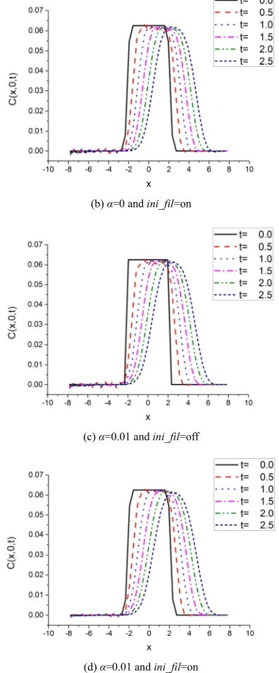
U ; α=0,0.01; ini_ fil=on,off ; bdw=3. (102)

Numerical results are shown in Figs. 3 and 4. The accuracy of the numerical results is very high. The numerical results coincide with the exact ones. The spurious oscillation in Fig. 4 is reduced by increasing M and N, but it invites serious increase of computation time and memory. As shown in Fig. 5, the initial density filter and/or artificial damping given by Eqs. (99) and (100), respectively, can reduce the spurious oscillation.

6.2. Application of GIRM to Burgers’ Equation

As a basis of discussion, we discuss the solution of one-dimensional Initial Boundary Value Problem (IBVP) of

d

N -dimensional Burgers’ equation.

If xi, (i=1,2,⋯,Nd) and t refer to the coordinates

and time, the fluid motion in Nd-dimension is expressed as

j j

i j

i j i

x x

u x

u u t u

∂ ∂

∂ = ∂ ∂ + ∂

∂ 2

ν , (103)

The summation convention is used for the repeated indices,

that is, 12 2 2

2 2

N i

i x x x

x∂ =∂ ∂ + +∂ ∂

∂

∂ ⋯ . ui ,

) , , 2 , 1

(i= ⋯ Nd refers to the velocity vector. ν is the

kinematic viscosity. Since it’s not difficult to obtain two-dimensional expressions from three-dimensional ones, we develop theory using three-dimensional expressions below.

We rewrite the basic equations Eq. (103) as follows: Non-uniformity equation:

j i j i

x u

∂ ∂ =

θ . (104)

Constitutive equation:

j i j i

q =−νθ . (105)

Equilibrium equation:

j j i j i j i

x q u

t u

∂ ∂ − = + ∂

∂ _θ

. (106)

We introduce Gaussian type Generalized Fundamental Solution (GFM) G~(x,ξ) with scale γi , (i=1,2,⋯,Nd)

[4,5]:

∏

= 

   

 

 ₋

− = Nd

i i

i

x G

1

2 2

2 ) ( exp 2

1 )

, ( ~

γ ξ γ

π

ξ

x , (107)

We obtain an integral representation of Eq. (104). From Eq. (107), we have

) , ( ~ ) , ( ) , ( ~ ) , ( ) , ( ~ ) , (

ξ x x ξ x x ξ

x x

j i j

i

j i

t u x

G t u G

x t

u _δ

− ∂

∂ = ∂

∂

(11)

where

) , ( ~ ) , ( ~

ξ x ξ x

i i x

G ₌_δ

∂ ∂

. (109)

∫∫∫

   

   

∂ ∂ − =

V

j i j

i G dV

x t u

t xξ x

x

x, ) ( , ) ~( , ) (

0 θ

∫∫∫

   

   

+ ∂

∂ − =

V i j

j i j

i u t dV

x G t u t

G x xξ x

ξ x x x

ξ

x ( , ) ( ,)~( , )

~ ) , ( ) , ( ) , (

~ _θ _δ

[

]

∫∫∫

+

=

V G xξ ij xt ui xt j(x,ξ)dVx

~ ) , ( ) , ( ) , (

~ _θ _δ

∫∫

−

Sui xt G(x,ξ)nxjdSx

~ ) ,

( . (110)

∫∫∫

=−

V i j

VG x ξ ij x t dVx u x t (x,ξ)dVx

~ ) , ( )

, ( ) , (

~ _θ _δ

∫∫

+

Sui xt G(x,ξ)nxjdSx

~ ) ,

( . (111)

Exchanging x and ξ in Eq. (111), we obtain a generalized integral representation for Eq. (106):

∫∫∫

=−

V i j

VG ξ x ij ξt dVξ u ξt (ξ,x)dVξ

~ ) , ( )

, ( ) , (

~ _θ _δ

∫∫

+

SG(ξ,x)ui(ξ,t)nξjdSξ

~

(112)

The generalized integral representation of Eq. (106) is obtained similarly. From Eq. (107), we have

) , ( ~ ) , ( ) , ( ~ ) , ( ) , ( ~ ) , (

ξ x x ξ

x x ξ

x x

j j i j

j i

j j i

t q x

G t q G

x t q

δ

− ∂

∂ = ∂

∂

. (113)

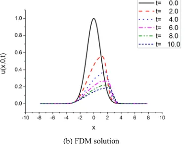
(a)Numerical solution

(b) Exact solution

Figure 3. Exponential initial density distribution (N=21, α=0, ini_fil=off).

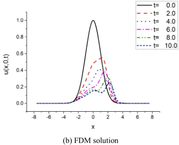
(a) Numerical solution

(b) Exact solution

Figure 4. Rectangular initial density distribution (N=41, α=0, ini_fil=off).

∫∫∫

   

   

∂ ∂ + +

∂ ∂ =

V

j j i j

i j i

dV x

t q t t u t

t u

G x

x x

ξ

x, ) ( ,) ( , ) ( , ) ( ,)

( ~

0 θ

∫∫∫



  

 

+ ∂ ∂ =

V j ij

i

dV t t u G t

t u

G xξ x x x

x ξ

x, ) ( , ) ~( , ) ( , ) ( , )

(

~ _θ

∫∫∫

_

 

   

− ∂

∂ +

V ij j

j j i

dV t

q x

t q G

x ξ x x x

ξ x

) , ( ~ ) , ( ) , ( ) , ( ~

δ

∫∫∫

+

∂ ∂ =

V j ij

V

i

dV t t u G dV

t t u

G x x ξ x x x

x ξ

x, ) ( , ) ~( , ) ( ,) ( , )

(