A Chaotic Modified Algorithm for Economic Dispatch Problems with Generator Constraints

http://www.sciencepublishinggroup.com/j/ajece doi: 10.11648/j.ajece.20170102.12

A Chaotic Modified Algorithm for Economic Dispatch

Problems with Generator Constraints

Mojtaba Ghasemi

Department of Electronics and Electrical Engineering, Shiraz University of Technology, Shiraz, Iran

Email address:

To cite this article:

Mojtaba Ghasemi. A Chaotic Modified Algorithm for Economic Dispatch Problems with Generator Constraints. American Journal of Electrical and Computer Engineering. Vol. 1, No. 2, 2017, pp. 61-71. doi: 10.11648/j.ajece.20170102.12

Received: March 23, 2017; Accepted: April 18, 2017; Published: June 8, 2017

Abstract:

The different Economic Dispatch (ED) problems have non-convex/non-smooth total fuel cost function with equality and inequality constraints which make it difficult to be effectively solved. Different heuristic optimization algorithms and stochastic search techniques have been proposed to solve ED problems in previous study. This paper proposes the Chaotic Modified Imperialist Competitive algorithms (CMICA) based on chaos maps to solve different ED problems in power systems. The proposed CMICA methods framework is applied to 10-, 15-, and 40-unit generator systems in order to evaluate its feasibility and efficiency. Simulation results demonstrate that the proposed CMICA methods were indeed capable of obtaining higher quality solutions efficiently in ED problem.

Keywords:

Economic Dispatch (ED) Problem, Generator Constraints, Imperialist Competitive Algorithm (ICA), Chaos Maps

1. Introduction

The main objective of Economic Dispatch (ED) problem is to allocate power demand among power systems generators in the most economical manner, while satisfying the operational and physical constraints as valve-point effects, prohibited operating zones, and multi-fuel options [1-2]. In the previous studies various classical optimization techniques and mathematical programming have been used. The classical optimization techniques are based on the assumption that the incremental cost of generator monotonically increases [3-13]. Classical methods are very sensitive to the choosing of the first point and therefore often they converge to a local optimum or even diverge with each other [14].

In the last few years, various evolutionary algorithms have been applied to solve ED optimization problem, such as Tabu Search (TS) [15], Genetic Algorithms (GA) [16-17], Particle Swarm Optimization (PSO) and Teaching–Learning-Based Optimization (TLBO) algorithms [18–25], Differential Evolution (DE) [26], Simulated Annealing (SA) [27], Hybrid GA (HGA) [28], combination of Biogeography-Based

Optimization (BBO) and DE (DE/BBO) [29-30],

Evolutionary Strategy Optimization (ESO) [31-32], hybrid

SA and PSO (SA-PSO) [1], the hybrid PSO algorithms (PSO-SQP) [33-34], Variable Scaling Hybrid Differential Evolution (VSHDE) [35], BBO algorithm [36], Hybrid Hopfield Neural Network Quadratic Programming based technique (HNN-QP) [37] and New PSO (NPSO) [38] have been used to solve ED problems. These methods have shown that can be efficiently used to eliminate most of the difficulties of classical ones.

ICA technique [39] is one of the modern heuristic optimization algorithms by Atashpaz-Gargari and Lucas in 2007. The performance and effectiveness of ICA algorithm have been continuously reinstated by successful utilization in many engineering applications [40-46]. In this paper, the effectiveness of the CMICA techniques has been demonstrated on three medium and large sized power systems with 10-, 15-, and 40-unit generator systems, respectively. The experimental results on the different ED problems have been compared to recently published results and found to be superior.

2. Formulation of ED Problems

constraints of a power system.

The basic objective function of basic ED problem can be mathematically formulated by a single quadratic function [1-2]:

2

1 1

cos ( )

g g

N N

i i i i i i i

i i

t F P a P b P c

= =

=

∑

=

∑

+ + (1)

Subject to:

Active power generation-demand balance: The total active power output of generating units of power system must be enough to meet the total load demand PD and power system total active power losses PL which is an equality constraint. The active power balance including losses is written as:

1

g

N

i D L

i

P P P

=

= +

∑

(2)

where network power losses PL can be calculated using loss

coefficients B as follows [29, 36]:

0 00

1 1 1

g g g

N N N

L i ij j i

i j i

P P B P B B

= = =

=

∑∑

+

∑

+ (3)

Generation limits: The active power output of each network generator limits will be:

,min ,max

i i i

P ≤ ≤P P (4) Ramp Rate Limits: The actual operating range of all the online units output should be in an acceptable range and is limited by the corresponding ramp rate limits, i.e.:

0 0

i i i i i i

P−P ≤UR and P − ≤P DR (5)

where P_i0 is the previous generation output of the ith generator; DR_iand UR_i are the down-ramp and up-ramp limits of the ith generator, respectively.

To consider the units output limits and ramp rate limits constraints at the same time, (4) and (5) can be rewritten as an inequality constraint as follows:

{

}

{

}

,min ,max

0 0 0 0

,min ,max ,min ,max

max , min ,

i i i

i i i i i i i i i i i i i

P P P

P P DR P P P UR P P UR and P P UR

≤ ≤

− ≤ ≤ + − ≤ − ≤ (6)

2.1. Objective Functions for ED Problem

2.1.1. ED Problem Considering Valve-Point Effects

In power systems, the generators with multi-valve stream turbines have Valve-Point Effects (VPE), the characterized in the form of a quadratic function plus the absolute value of a sinusoidal term corresponding to the VPE [45]. The objective function of this problem can be formulated as follows:

2

, min

1 1

cos ( ) sin( ( ))

g g

N N

i i i i i i i i i i i

i i

t F P a P b P c e f P P

= =

=

∑

=

∑

+ + + × × − (7)

2.1.2.ED Problem Considering Multiple Fuels

Also, in practical power system operation conditions, any given unit with Multiple Fuel (MF) cost curves needs to operate on the lower contour of the intersecting curves. Therefore, unlike the conventional total fuel cost function, the fuel cost function of each power generating units should be presented with a few piecewise functions reflecting the effect of fuel type changes such as oil, natural gas and coal [2]. The costs function considering multi-fuel of unit ith is represented in [46] and as follows:

2

1 1 1 ,min 1

2

2 2 2 1 2

2

1 ,max

, 1,

, 2,

( ) ...

, ,

i i i i i i i i

i i i i i i i i

i i

ij i ij i ij ij i i

a P b P c fuel P P P

a P b P c fuel P P P

F P

a P b P c fuel j P₋ P P

 _{+ + ≤ ≤}



 _{+ + ≤ ≤}

 =  

+ + ≤ ≤



(8)

2.1.3.ED Problem Considering Prohibited Operating Zones The input–output curve of practical thermal generating units may have Prohibited Operating Zones (POZ) because of

faults in the generators themselves or in the associated auxiliaries such as feed pumps, boilers, etc [1, 2]. The POZ constraints can be described as follows:

,min 1

1

,max

; 2,..., ;

i

l

i i i

u l

i ik i ik i

u

in i i

P P P

P P P P k n i

P P P

−

 _{≤ ≤}



∈ ≤ ≤ = ∀ ∈ Ω 

≤ ≤ 

(9)

The equation (9) indicates that if ith generator and niis the

number of POZ of the ith generator, it will have (ni+1)

feasible disjoint operating regions which will form a non-convex set.

3. Proposed ICA Method

3.1. ICA Method

fundamental concepts about these proposed algorithms. ICA technique, proposed by Atashpaz and Lucas [39]. The ICA method has proven its superior capabilities and effectiveness, such as better global minimum achievement and faster convergence, applicability in various domains are currently being extensively investigated [40-44].

3.1.1. Generating Initial Empires

The goal of optimization is to find and optimal solution in terms of variable values which should be optimized. In ICA technique, a country is a 1 × Nvar array which is defined as follow:

var

1 2 3

[ , , ,..., _N ]

country= P P P P ₍₁₀₎

where Pis are considered as the variables of the cost function that should be optimized.

The country includes a combination of some socio-political characteristics such as, welfare, culture, economic and academic education.

The optimal solution is the maximum power (minimum cost) which can found by evaluating the cost of a country as follow,

var

1 2 3

costi=f country( )=f P P P( , , ,...,PN ) (11)

In the first step of this technique, ICA algorithm starts with a randomly initial population of size Ncountry. T he Nimp is selected from the strongest initial countries to form the empires, and the remaining Ncol of the initial countries will form the colonies. The normalized cost of an imperialist state to divide the colonies among imperialists is explained as follows:

max{ }

n i n

i c c

C

= −

(12)

where c_n is the cost of nth imperialist and C_n is the normalized cost which is the portion of colonies that must be possessed by the imperialist. The normalized power of each imperialist's state can be evaluated as follows:

1

imp

n

n N

i i

C P

C

= =

∑

(13)

To divide the early colonies among the imperialist by their power, some of initial colonies are given to each imperialist. The initial colonies are distributed among empires according to their power, so, the initial number of colonies for nth empire can be explained as follows,

. ._n { _n. _col}

N C =round P N (14) where N. C. n factor is the initial population number of colonies of the empire and Ncol presents the total number of existing colonies countries in the initial countries crowds,

where the bigger and powerful empires have greater number of colonies and weaker empires have less number of colonies.

3.1.2. Absorption Policy Modeling

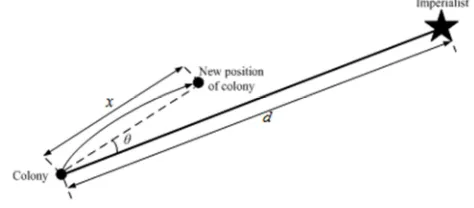
The imperialist states tried to absorb their colonies and make them a part of themselves by pursuing assimilation policy. In other words, the central government attempts to close colony country to its own imperialist by applying attraction policy. More precisely, imperialist states force their colonies to move toward themselves along different socio-political axis. In the ICA, this process is modelled by moving all of the colonies toward the imperialist along different optimization axis. In Figure 1, d is distance among colony and imperialist who presents distance between imperialist and colony countries, and x is the accidental number with steady distribution, and θ is a random number with uniform distribution. The x variable can be defined as follows:

~ (0 , )

x U

β

×d (15) where β is an assimilation factor which can be a number bigger than one and nears to two, and a good selection can be

β=2. The θ parameteris defined as follows:

~ (U , )

θ

−

γ

+

γ

(16)

where γ is a vector and its elements are uniformly distributed random numbers between zero and one, which is an ideal parameter that its growth causes increasing in searching area around imperialist and reduction of its value causes colonies close possibly to the vector of connecting colony to the imperialist, and usually the value of γ is arbitrary and about π/5 (Rad).

Figure 1. Giving a move to the colonies toward their corresponding imperialist in an accidental deviated orientation.

3.1.3. Total Power of an Empire

Total power of an empire is mainly related by the power of imperialist country; however the power of colonies of an empire has a little effect on the sum power. The sum cost of an empire depends on the power of imperialist and its colony by considering of the both above mentioned factors that can be calculates as follow,

. ._n ( _n) { ( _n)}

T C =Cost imperialist +ξmean Cost colonies of empire (17)

which the power of colonies on the empire power is tuned by it, is a positive number that has value between zero and one and near to zero. The value of 0.15 for ξ has shown good balanced results in most of the implementations.

3.1.4. Imperialistic Competitions

This competition is modelled by just choosing the weakest colony of empire and making a competition among all empires. Finally, the most powerful empires take possession of others. In the first step of modeling of the competition between the empires for possessing these colonies, the weakest empire is selected to start the competition. Then the possession probability of each empire (PP) is estimated proportional to the total power of the empire. The normalized total cost of an empire is determined by:

. max{ . . } . .

. .

_{n i n}

i

C T C T C

N T

= − ₍₁₈₎

where T. C. n is total cost of nth empire and N. T. C. n is normalized cost of that nth empire.

By having the normalized total cost, the possession probability of each empire is defined by:

1 . . . . . . n _imp n p N i i

N T C P

N T C

= =

∑

(19)

Next, the mentioned colonies will be divided accidentally between the empires with a certain probability. In order to divide the given colonies among the empires, vector P is formed as follows:

1, 2, 3,..., Nimp

p p p p

P=_P P P P _ (20)

After that, the vector R should be defined with the same size of vector P, and the arrays of this vector are accidental number with the same distribution in [1].

1, , ,...,2 3 Nimp

R=_r r r r _ (21)

Then, vector D is constructed by subtracting R from P.

1 2

1, 2,..., Nimp p 1, p 2,..., pNimp Nimp

D=P R- =_D D D _=__p −r p −r p −r _ (22)

3.2. Chaos Maps

The choice of chaotic sequences is justified theoretically by their unpredictability. The nature of chaos is apparently random and unpredictable, and mathematically, it is randomness of a simple deterministic dynamical system and can be considered as sources of randomness [47, 48]. Table 1 describes ten distinguished 1-D maps, in which the k means the index of the chaotic sequence, and xk represents the k

th

number in the chaotic sequence.

3.3. CICA Method

New algorithms called chaotic algorithms can be created by using chaotic behavior [49-50]. The random-based optimization algorithms which use chaotic variables are called Chaotic Optimization Algorithm (COA). The COA technologies can accomplish overall searches at higher speeds than stochastic searches that depend on probabilities, due to the non-repetition and periodicity of chaos [48-56]. In CICA way, the entire colony move towards their imperialist with a constant speed that increases the probability of the algorithm being trapped in a local optimum. And therefore, the choice of the initial value of β in the algorithm will be very important and also one of the important characteristics of chaotic algorithms is having the less sensitivity to the initial value. In this paper, for enhancing the performance of ICA algorithm and reducing the sensitivity to initial value of the β, chaotic variables are used. As a result, the equation of motion of the imperial colonies can be rewritten as follows:

1

( ) ( )

( ) ( ( ) ( ))

new old

k new old

d

Position Colony Position Colony

x₊ Colony β Position Imperialist Position Colony

=

+ ∗ ∗ − (23)

Table 1. Chaotic sequences [78-82] for CMICA method.

Map name Method Definition Details

Logistic CMICA/M1 xk+1=αxk(1−xk) α = 4; x0

∈ (0, 1) and x0 ≠ {0.0,

0.25, 0.75, 0.5, 1.0}

Cusb CMICA/M2 0.5

1 1 (2 )

k k

x₊ = − ∗x -

Sinus CMICA/M3 2sin( )

1 2.3( k)

x k k

x+ = x π -

Tent CMICA/M4 1

0.7 0.7

10

(1 ) 0.7

3 k k k k k x x x x x +  <  =  _{− ≥}  -

Gaussian CMICA/M5 1

0 0 1 mod(1) k k k x x otherwise x + =   =  

1 1 1

mod(1)

k k k

x x x

 

= −   

Singer CMICA/M6

2 1

3 4

(7.86 23.31 28.75 13, 3028.75 )

k k k

k k

x x x

x x

µ

+ = −

+ −

where µ is a control parameter, and is between 0.9 and 1.08.

Cubic CMICA/M7 2

1 (1 )

k k k

Map name Method Definition Details

Circle CMICA/M8 xk+1=xk+ −β α π( / 2 ) sin(2πxk) mod(1) With α = 0.5 and β = 0.2.

Chebyshev CMICA/M9 1

1 cos( cos ( ))

k k

x₊ = k − x -

Sinusoidal CMICA/M10 2

1 sin( )

k k k

x₊ =αx πx With α = 2.3.

3.4. Modified CICA Method

Another important tip on ICA algorithm is the movement of colony towards its imperialist which are not affected by the colonies of its own imperialist. In this paper, some of the colonies move towards their imperialist in a way that they

can be affected by other colonies of their own imperialist. Actually, in the modified algorithm, the imperialists try to reduce the average distance of their colonies and pull the whole set towards them. The equation of this motion can be shown as follow,

. . 1

1

( ) ( )

1

( ) ( ( ) ( ))

. .

n

mean

new old

N C

k new n i

n i

d

Position Colony Position Colony

x Colony Position Imperialist Position Colony

N C β

+

= =

∗

+ ∗ −

∑

(24)

and the general equation of absorbing colonies by their imperialist is as follows:

1

1

( ) ( ) ( )

( ( ) ( )), 0.35

( ) ( ) ( )

1

( ( )

. .

new old k new

old

new old k new

n

Position Colony Position Colony x Colony

Position Imperialist Position Colony if rand

Position Colony Position Colony x Colony

Position Imperialist

N C

β

β +

+

= + ∗

− ∗

− ∗

>

= + ∗

. .

1

( )), .

n

N C

i n _i

Position Colony otherwise

=

       



∑

(25)

4. Simulation Results

In this section of study, the CMICA methods have been applied to different ED problems in three different test cases (10, 15, and 40 thermal units). The initial population size of all proposed methods were fixed as 100, the maximum iteration number was set as 600. Generally, in order to employ CMICA algorithms on different ED problems, we should follow the below procedure:

Step 1: Calling the needed information for power system and CMICA algorithm.

Step 2: Production of chaotic algorithm’s initial population of countries.

Step 3: Calculation of ED problem objective function with imposing the constrained different ED problems, power generation-demand balance and the power limit constraint, for every available answer in population of initial countries of CMICA. The flowchart of constraint-handling procedure is given in [68].

Step 5: Selection of empires and distributing population of initial countries on empires with consideration to calculated normalized value of objective function in previous step.

Step 6: Movement of colonies towards imperialists and absorption action.

Step 7: Position replacement between imperialists and colony with consideration to calculated normalized value of objective function.

Step 8: Imperialistic competition between empires, fall of weak empire and repeat of 6th to 8th steps until end of total number of repetitions.

4.1. Case A: ED Problem Considering VPE and MFs

The first test system of simulation, which consists of 10 generators, is an ED problem with both valve point effects and multiple fuels supplying to a load demand of 2700 MW [67].

The fuel cost function of thermal unit ith can be expressed as:

2

1 1 1 1 1 1, min ,min 1

2

2 2 2 2 2 2, min 1 2

2

, min 1 ,max

sin( ( )) , 1,

sin( ( )) , 2,

( ) ...

sin( ( )) , ,

i i i i i i i i i i i i

i i i i i i i i i i i i

i i

ij i ij i ij ij ij ij i ij i i

a P b P c e f P P fuel P P P

a P b P c e f P P fuel P P P

F P

a P b P c e f P P fuel j P₋ P P

 _{+ + + × × − ≤ ≤} 

 _{+ + + × × − ≤ ≤} 

=

+ + + × × − ≤ ≤

  

(26)

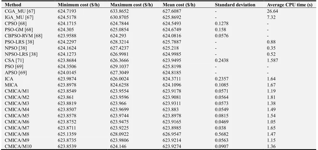
The comparison between best results using CMICA algorithm are shown in Table 2. For this test system, the best

efficiency results of the fuel cost minimum, the fuel cost maximum, the fuel cost mean, the standard deviations and the average CPU time (s) among the 50 runs of solutions satisfying the system constraints obtained by the proposed CMICA algorithms for 10 thermal units test system are

compared to those from other previous reported results such as CGA-MU [67], CBPSO-RVM [68], NPSO-LRS [38] and CSA [71], as shown in Table 3. It is clearly visible that the proposed CMICA algorithms outperform all previous reported algorithms in terms of achieving the fuel cost.

Table 2. Best solutions obtained by proposed ICA algorithms for 10 unit system (case A).

Unit Fuel

Unit power output (MW)

ICA MICA

Chaotic MICA methods CMICA/

M1

CMICA/ M2

CMICA/ M3

CMICA/ M4

CMICA/ M5

CMICA/ M6

CMICA/ M7

CMICA/ M8

CMICA/ M9

CMICA/M 10

1 2 221.6751 218.594 219.6265 217.567 217.5663 219.6223 220.648 217.567 218.594 210.6986 218.594 216.542

2 1 210.4739 211.9593 210.4739 210.7215 209.7312 209.9788 210.7215 213.1971 212.4544 205.6421 212.2069 211.9593

3 1 279.6493 279.5828 279.6489 281.6651 280.6562 280.6571 278.6406 281.6653 279.6489 279.7871 279.6489 282.6732

4 3 237.2207 240.9831 239.6394 239.3707 240.0425 240.0425 239.3707 240.8488 239.1019 240.9954 241.5206 240.58

5 1 275.9598 275.8557 279.8774 279.6876 282.2783 280.0155 279.9505 280.5375 276.9936 280.5915 280.0039 280.2367

6 3 240.9831 239.1019 239.2363 238.6988 240.1769 240.4457 240.1769 240.8488 240.3113 241.087 239.5051 239.1019

7 1 292.4704 287.4507 292.4696 287.6959 287.5789 287.728 287.7277 287.794 292.4697 299.1469 290.0985 287.7505

8 3 241.5206 240.4457 240.7144 240.8488 240.58 239.1019 240.1769 239.1019 240.7144 234.6658 239.1019 239.6394

9 3 421.2979 426.6803 425.5196 427.1749 425.4462 426.4931 426.3422 425.6264 423.8219 417.3747 422.9117 425.4072

10 1 278.7482 279.3465 272.7677 276.5697 275.9403 275.914 276.245 272.8132 275.888 289.9813 276.4085 276.1058

Total cost ($) 623.9874 623.8978 623.8549 623.861 623.8819 623.8507 623.8578 623.8752 623.8711 625.1359 623.8735 623.8539

Table 3. Comparison of best solutions obtained by proposed ICA algorithms and reported solutions for 10 unit system.

Method Minimum cost ($/h) Maximum cost ($/h) Mean cost ($/h) Standard deviation Average CPU time (s)

CGA_MU [67] 624.7193 633.8652 627.6087 - 26.64

IGA_MU [67] 624.5178 630.8705 625.8692 - 7.32

CPSO [68] 624.1715 624.7844 624.5493 0.1278 -

PSO-GM [68] 624.305 625.0854 624.6749 0.158 -

CBPSO-RVM [68] 623.9588 624.293 624.0816 0.0576 -

PSO-LRS [38] 624.2297 628.3214 625.7887 - 0.88

NPSO [38] 624.1624 627.4237 625.218 - 0.35

NPSO-LRS [38] 624.1273 626.9981 624.9985 - 0.52

CSA [71] 623.8684 626.3666 623.9495 0.2438 1.587

PSO [69] 624.3506 629.1037 625.8198 - -

APSO [69] 624.0145 627.3049 624.8185 - -

ICA 623.9874 626.0024 824.3711 0.2357 1.64

MICA 623.8978 824.6258 624.1096 0.1085 1.67

CMICA/M1 623.8549 623.9554 623.9178 0.0571 1.19

CMICA/M2 623.861 623.9596 623.9081 0.0564 1.81

CMICA/M3 623.8819 623.966 623.9311 0.0573 1.38

CMICA/M4 623.8507 623.9699 623.883 0.0549 1.49

CMICA/M5 623.8578 623.9744 623.8978 0.0815 1.54

CMICA/M6 623.8752 623.9475 623.9165 0.0469 1.05

CMICA/M7 623.8711 623.9225 623.8985 0.038 1.65

CMICA/M8 625.1359 628.0922 626.9547 0.5682 1.47

CMICA/M9 623.8735 623.9806 623.9214 0.0563 1.15

CMICA/M10 623.8539 624.146 623.9274 0.0907 1.36

The convergence characteristics for proposed CICA algorithms of 10 unit test system for ED problem for case A are shown in Figure 2.

Figure 2. Convergence characteristics of proposed algorithms for 10 unit system (case A).

0 100 200 300 400 500 600

624 625 626 627 628 629 630 631 632

Iteration

M

in

im

u

m

c

o

st

(

$

/h

)

4.2. Case B: ED Problem Considering Generators

Prohibited Operating Zones and Transmission Network Power Losses

The case B of simulation for ED problem consists of 15 generators and is a network with power system thermal units prohibited operating zones and transmission network power losses supplying to a load demand of 2630 MW [74].

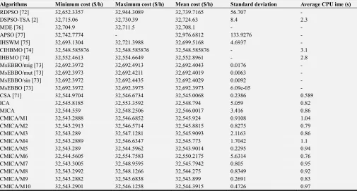
The best solutions of generation output of each system unit using proposed ICA algorithms are provided and shown in Table 4, the best of minimum total fuel cost is $/h

32,543.2882 using CMICA method based on Chebyshev map (CMICA/M9). Comparison of simulation results using proposed algorithms and previous reported results best for 15 unit system (case B) are shown in Table 5, the best previous reported results is $/h 32,544.9704 using proposed CSA [71] method. The proposed CMICA algorithms perform better than original ICA algorithm in all accounts. Amongst all the reported results, proposed CMICA algorithms yield better results than previous listed algorithms in all accounts.

Table 4. Best solutions obtained by proposed CMICA algorithms for 15 unit system (case B).

Unit

Units power output (MW) Chaotic MICA methods

CMICA/M1 CMICA/M2 CMICA/M3 CMICA/M4 CMICA/M5 CMICA/M6 CMICA/M7 CMICA/M8 CMICA/M9 CMICA/M10

1 455 455 455 455 455 455 455 455 455 455

2 455 455 455 455 455 455 455 455 455 455

3 130 130 130 130 130 130 130 130 130 130

4 130 130 130 130 130 130 130 130 130 130

5 231.5103 232.3193 231.4876 231.7559 231.4876 229.6902 233.3073 232.9779 231.4839 231.7684

6 460 460 460 460 460 456.5507 460 460 460 460

7 465 465 465 465 465 465 465 465 465 465

8 60 60 60 60 60 60 60 60 60 60

9 25 25 25 25 25 25 25 25 25 25

10 35.715 35.3739 35.5584 35.5414 35.5584 41.1988 34.0864 35.3901 35.4436 35.713

11 74.0987 73.6505 74.2783 74.033 74.2783 73.8171 73.9789 72.9905 74.3972 73.8484

12 80 80 80 80 80 80 80 80 80 80

13 25 25 25 25 25 25 25 25 25 25

14 15 15 15 15 15 15 15 15 15 15

15 15 15 15 15 15 15 15 15 15 15

Losses

(MW) 26.3241 26.3438 26.3243 26.3303 26.3243 26.2635 26.3726 26.3586 26.3248 26.3298

Total cost

($/h) 32,543.2888 32,543.2913 32,543.289 32,543.2889 32,543.289 32,544.5605 32,543.3005 32,543.2992 32,543.2882 32,543.2901

Table 5. Comparison of best solutions obtained by proposed ICA algorithms and reported best solutions for 15 unit system.

Algorithms Minimum cost ($/h) Maximum cost ($/h) Mean cost ($/h) Standard deviation Average CPU ime (s)

RDPSO [72] 32,652.3357 32,944.3089 32,739.7165 56.707 -

DSPSO-TSA [2] 32,715.06 32,730.39 32,724.63 8.4 2.3

MDE [76] 32,704.9 32,711.5 32,708.1 - -

APSO [77] 32,742.7774 - 32,976.6812 133.9276 -

IHSWM [75] 32,693.1304 32,721.3988 32,699.5168 4.6937 -

CIHBMO [74] 32,548.585876 32,548.585876 32,548.585876 - 3.1

IHBMO [74] 32,552.4613 32,554.6649 32,552.8961 - 2.8

MsEBBO/mig [73] 32,692.3972 32,692.4913 32,692.4043 0.0176 -

MsEBBO/mut [73] 32,692.3973 32,692.4211 32,692.4019 0.0063 -

MsEBBO/sin [73] 32,692.3972 32,692.4435 32,692.4029 0.0092 -

MsEBBO [73] 32,692.3972 32,692.3975 32,692.3973 6.09e-05 -

CSA [71] 32,544.9704 32,546.6734 32,545.0068 0.2386 0.589

ICA 32,545.8185 32,553.3592 32,548.794 5.059 0.82

MICA 32,544.559 32,548.2506 32,546.0017 3.416 0.86

CMICA/M1 32,543.2888 32,546.6852 32,545.924 0.9108 1.04

CMICA/M2 32,543.2913 32,546.5714 32,545.8815 0.8275 0.79

CMICA/M3 32,543.289 32,547.1281 32,545.9093 2.1163 0.86

CMICA/M4 32,543.2889 32,546.6347 32,545.773 1.7042 1.1

CMICA/M5 32,543.289 32,544.5962 32,543.9014 0.2295 0.94

CMICA/M6 32,544.5605 32,554.7583 32,550.2175 5.6314 0.76

CMICA/M7 32,543.3005 32,548.9595 32,545.7942 0.805 0.95

CMICA/M8 32,543.2992 32,548.1266 32,544.275 0.8349 0.92

CMICA/M9 32,543.2882 32,545.6838 32,543.899 0.2691 0.83

4.3. Case C: ED Problem Considering Valve Point Effects Using Large-Scale Generating System

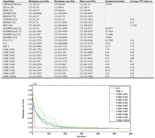
In case C of simulation, the CMICA algorithms have been applied to the ED problem with 40-generating unit, the system is presented in [16].

The results best for CMICA algorithms are provided in Tables 6. According to Table 6, it can be observed that the

best results obtained by ICA algorithms is $/h 121,412.5376 which is obtained by the proposed CMICA/M2 method. The CMICA algorithms always provide the same solution in more simulations, which shows the reliability of the proposed methods. The convergence performance of ICA algorithms for 40-unit test system plotted in Figure 3.

Table 6. Comparison of best solutions obtained by proposed ICA algorithms and reported best solutions for 40 unit system.

Algorithms Minimum cost ($/h) Maximum cost ($/h) Mean cost ($/h) Standard deviation Average CPU time (s)

CBPSO-RVM [68] 121,555.32 123,094.98 122,281.14 259.99 -

DEvol [70] 121,412.91 121,464.4 121,430.0 - -

MDE [76] 121,414.79 121,466.04 121,418.44 - -

DE/BBO [29] 121,420.8948 121,420.8963 121,420.8952 -

IHSWM [75] 121,412.57 121,415.78 121,413.3879 - -

CIHBMO [74] 121,412.57 121,412.63 121,412.5919 - 16.8

IHBMO [74] 121,517.8 121,711.8526 121,589.1827 - 15.2

BBO [36] 121,426.953 121,688.6634 121,508.0325 - 1.1749

MsEBBO/mig [73] 121,415.52 121,521.6899 121,476.2517 36.4077 -

MsEBBO/mut [73] 121,416.2885 121,585.0186 121,500.9279 32.7428 -

MsEBBO/sin [73] 121,415.309 121,479.3657 121,421.6556 11.5696 -

MsEBBO [73] 121,412.5344 121,450.0026 121,417.1877 5.7996 -

CSA [71] 121,412.5355 121,810.2538 121,520.4106 63.5705 3.03

ICA 121,425.6295 121,680.6004 121,515.8134 54.32 3.93

MICA 121,419.9407 121,505.1538 121,432.524 43.17 3.75

CMICA/M1 121,422.7704 121,428.9514 121,424.2761 1.76 4.18

CMICA/M2 121,412.5376 121,414.265 121,413.0084 0.85 4.58

CMICA/M3 121,412.5421 121,416.3812 121,414.075 0.82 3.62

CMICA/M4 121,412.5421 121,414.4127 121,412.8592 0.97 4.05

CMICA/M5 121,412.541 121,415.7735 121,413.2618 0.74 4.2

CMICA/M6 121,434.2654 121,474.985 121,445.2107 4.58 3.69

CMICA/M7 121,412.5421 121,414.6913 121,414.0204 0.66 4.14

CMICA/M8 121,416.2547 121,901.5275 121,518.4232 40.12 3.94

CMICA/M9 121,412.5452 121,415.886 121,412.9415 1.03 4.05

CMICA/M10 121,412.5445 121,414.7892 121,412.7604 0.53 3.72

Figure 3. Convergence characteristics of proposed algorithms for 40 unit system (case C).

5. Conclusion

This paper proposes CMICA algorithms based on different chaotic maps for solving ED problems. Many nonlinear characteristics of the ED problems. The comparative and application studies of different chaotic maps have been done

for improving the global searching capability and escaping from a local minimum of ICA method. The simulation results clearly demonstrated that proposed CMICA algorithms which are capable of achieving global solutions is simple with computationally efficient and has stable and better dynamic convergence characteristics.

0 100 200 300 400 500 600

1.2 1.22 1.24 1.26 1.28 1.3 1.32 1.34 1.36 1.38

1.4x 10

5

Iteration

M

in

im

u

m

c

o

st

(

$

/h

)

References

[1] R. Azizipanah-Abarghooee, T. Niknam, M. Gharibzadeh, and F. Golestaneh, “Robust, fast and optimal solution of practical economic dispatch by a new enhanced gradient-based simplified swarm optimisation algorithm,” IET Gener. Transm. Distrib., vol. 7, no. 6, pp. 620–635, Jun. 2013. [2] Niknam T. A new fuzzy adaptive hybrid particle swarm

optimization algorithm for linear, smooth and non-convex economic dispatch problem. Appl Energ 2010; 87 (1): 327–39.

[3] M. Ghasemi, J. Aghaei, E. Akbari, S. Ghavidel, and L. Li, “A differential evolution particle swarm optimizer for various types of multi-area economic dispatch problems,” Energy, vol. 107, pp. 182–195, 2016.

[4] Bakirtzis A, Petridis V, Kazarlis S. Genetic algorithm solution to the economic dispatch problem. Proc Inst Electr Eng Gen Trans Dist 1994; 141: 377–82.

[5] Lee FN, Breipohl AM. Reserve constrained economic dispatch with prohibited operating zones. IEEE Trans Pow Syst 1993; 8: 246–54.

[6] Yoshida H, Kawata K, Fukuyama Y, Takayama S, Nakanishi Y. A particle swarm optimization for reactive power and voltage control considering voltage security assessment. IEEE Trans Pow Syst 2000; 15: 1232–9.

[7] Naka S, Genji T, Yura T, Fukuyama Y. Practical distribution state estimation using hybrid particle swarm optimization. Proc IEEE Pow Eng Soc Winter Meet 2001; 2: 815–20. [8] Chen JF, D Chen S. Multi objective power dispatch with line

flow constraints using the fast Newton–Raphson method. IEEE Trans Energ Convers 1997; 12: 86–93.

[9] Hindi KS, Ab Ghani MR. Dynamic economic dispatch for large-scale power systems: a lagrangian relaxation approach. Electr Pow Syst Res 1991; 13: 51–6.

[10] Liang ZX, Glover JD. A zoom feature for a dynamic programming solution to economic dispatch including transmission losses. IEEE Trans Pow Syst 1992; 7: 544–50. [11] Jabr R, Coonick A, Cory B. A homogeneous linear

programming algorithm for the security constrained economic dispatch problem. IEEE Trans Pow Syst 2000; 15: 930–7. [12] Papageorgiou LG, Fraga ES. A mixed integer quadratic

programming formulation for the economic dispatch of generators with prohibited operating zones. Electr Pow Syst Res 2007; 77: 1292–6.

[13] Takriti S, Krasenbrink B. A decomposition approach for the fuel constrained economic power-dispatch problem. Eur J Oper Res 1999; 112: 460–6.

[14] Abdollahi A, Ehsan M, Rashidinejad M, Pourakbari-kasmaei M. Cost-based unit commitment considering prohibited zones and reserve uncertainty. Int Rev Electr Eng 2009; 4(3): 425– 33.

[15] Lin VM, Cheng FS, Tsay MT. An improved tabu search for economic dispatch with multiple minima. IEEE Trans Power Syst 2002; 17 (1): 108–12.

[16] Chen PH, Chang H-C. Large-scale economic dispatch by

genetic algorithm. IEEE Trans Power Syst 1995; 10 (4): 1919–26.

[17] Baskar S, Subbaraj P, Rao MVC. Hybrid real coded genetic algorithm solution to economic dispatch problem. Comput Electr Eng 2003; 29 (3): 407–19.

[18] Park JB, Lee K-S, Shin J-R, Lee KY. A particle swarm optimization for economic dispatch with non-smooth cost functions. IEEE Trans Power Syst 2005; 20 (1): 34–42. [19] M. Ghasemi, M. M. Ghanbarian, S. Ghavidel, S. Rahmani, E.

Mahboubi- Moghaddam, Modified teaching learnin galgorithm and double differential evolution algorithm for optimal reactive power dispatch problem: a comparative study, Inf. Sci. 278(2014) 231–249.

[20] Yuan X, Su A, Yuan Y, Nie H, Wang L. An improved PSO for dynamic load dispatch of generators with valve-point effects. Energy 2009; 34 (1): 67–74.

[21] Niknam T, Mojarrad HD, Meymand HZ. A new particle swarm optimization for non-convex economic dispatch. Eur Trans Electr Power 2011; 21(1): 656–79.

[22] M. Ghasemi, S. Ghavidel, M. Gitizadeh, and E. Akbari, “An improved teaching–learning-based optimization algorithm using Levy mutation strategy for non-smooth optimal power flow,” Int. J. Electr. Power Energy Syst. 65, 375 (2015). [23] Chaturvedi KT, Pandit M, Srivastava L. Self-organizing

hierarchical particle swarm optimization for nonconvex economic dispatch. IEEE Trans Power Syst 2008; 23(3): 1079–87.

[24] Meng K, Wang HG, Dong ZY, Wong KP. Quantum-inspired particle swarm optimization for valve-point economic load dispatch. IEEE Trans Power Syst 2010; 25(1): 215–22. [25] Ghasemi M, Taghizadeh M, Ghavidel S et al (2015) Solving

optimal reactive power dispatch problem using a novel teaching–learning-based optimization algorithm. Eng Appl Artif Intell 39: 100–108.

[26] Subbaraj P, Rengaraj R, Salivahanan S. Enhancement of combined heat and power economic dispatch using self adaptive real-coded genetic algorithm. Appl Energy 2009; 86 (6): 915–21.

[27] Wong KP, Wong YW. Genetic and genetic/simulated-annealing approaches to economic dispatch. IEE Proc Gen Transm Distrib 1994; 141 (5): 507–13.

[28] He DK, Wang FL, Mao ZZ. Hybrid genetic algorithm for economic dispatch with valve-point effect. Electr Power Syst Res 2008; 78 (4): 626–33.

[29] Bhattacharya A, Chattopadhyay PK. Hybrid differential evolution with biogeography-based optimization for solution of economic load dispatch. IEEE Trans Power Syst 2010; 25 (4): 1955–64.

[30] dos Santos Coelho L, Mariani VC. Combining of chaotic differential evolution and quadratic programming for economic dispatch optimization with valve-point effect. IEEE Trans Power Syst 2006; 21 (2); 989–96.

[32] Swarup KS, Kumar PR. A new evolutionary computation technique for economic dispatch with security constraints. Int J Electr Power Energy Syst 2006; 28 (4): 273–83.

[33] Victoire TAA, Jeyakumar AE. Hybrid PSO-SQP for economic dispatch with valve-point effect. Electr Power Syst Res 2004; 71 (1): 51–9.

[34] Vlachogiannis JG, Lee KY. Economic load dispatch – a comparative study on heuristic optimization techniques with an improved coordinated aggregation-based PSO. IEEE Trans Power Syst 2009; 24 (2): 991–1001.

[35] Ashwani K, Wenzhong G. Pattern of secure bilateral transactions ensuring power economic dispatch in hybrid electricity markets. Appl Energy 2009; 86 (7–8): 1000–10. [36] Bhattacharya A, Chattopadhyay PK. Biogeography-based

optimization for different economic load dispatch problems. IEEE Trans Power Syst 2010; 25 (2): 1064–77.

[37] Mekhamer SF, Abdelaziz AY, Kamh MZ, Badr MAL. Dynamic economic dispatch using a hybrid Hopfield neural network quadratic programming based technique. Electr Power Compon Syst 2009; 37 (3): 253–64.

[38] Selvakumar AI, Khanushkodi T. A new particle swarm optimization solution to non-convex economic dispatch problems. IEEE Trans Power Syst 2007; 22 (1): 42–51. [39] Atashpaz-Gargari E, Lucas C. Imperialist competitive

algorithm: an algorithm for optimization inspired by imperialistic competition. Proc. IEEE Congress on Evolutionary Computation 2007; pp. 4661–7.

[40] Ghasemi M, Ghavidel S, Ghanbarian MM, Gitizadeh M. Multi-objective optimal electric power planning in the power system using Gaussian bare-bones imperialist competitive algorithm. Inform Sci 2014; 294: 286–304.

[41] M. Ghasemi, S. Ghavidel, M. M. Ghanbarian, et al., Application of imperialist competitive algorithm with its modified techniques for multi-objective optimal power flow problem: a comparative study, Inf. Sci. 281 (2014)225–247. [42] M. Ghasemi, S. Ghavidel, M. M. Ghanbarian, et al.,

Multi-objective optimal power flow considering the cost, emission, voltage deviation and power losses using multi-objective modified imperialist competitive algorithm, Energy 78 (2014) 276–289.

[43] Ghasemi M, Ghavidel S, Rahmani S, Roosta A, Falah H. A novel hybrid algorithm of imperialist competitive algorithm and teaching learning algorithm for optimal power flow problem with non-smooth cost functions. Eng Appl Artif Intell 2014; 29: 54–69.

[44] Ghasemi M, Roosta A. Imperialist competitive algorithm for optimal reactive power dispatch problem: a comparative study. J World’s Electr Eng Technol 2013; 2: 13–20.

[45] M. Ghasemi, M. Taghizadeh, S. Ghavidel, A. Abbasian, Colonial competitive differential evolution: An experimental study for optimal economic load dispatch, Applied Soft Computing 40 (2016) 342–363.

[46] Ghasemi M, Ghavidel S, Ghanbarian MM, Habibi A. A new hybrid algorithm for optimal reactive power dispatch problem with discrete and continuous control variables. Appl Soft Comput 2014; 22: 126–40.

[47] Schuster HG. Deterministic chaos: An introduction (2nd revised ed.). Federal Republic of Germany: Physick-Verlag, GmnH, Weinheim, 1988.

[48] Coelho L, Mariani VC. Use of chaotic sequences in a biologically inspired algorithm for engineering design optimization. Expert Syst Appl 2008; 34: 1905–13.

[49] Xu H, Zhu H, Zhang T, Wang Z. Application of mutation scale chaos algorithm in power plant and units economics dispatch. J Harbin Inst Tech 2000; 32(4): 55–8.

[50] Xu L, Zhou S, Zhang H. A hybrid chaos optimization method and its application. System Eng Electron 2003; 25(2): 226–8. [51] Gong W, Wang S. Chaos ant colony optimization and

application. In: 4th International Conference on Internet Computing for Science and, Engineering, 2009; pp. 301–3. [52] Alatas B. Chaotic bee colony algorithms for global numerical

optimization. Expert Syst Appl 2010; 37: 5682–7.

[53] Alatas B, Akin E, Bedri Ozer A. Chaos embedded particle swarm optimization algorithms. Chaos Soliton Fract 2009; 40 (4): 1715–34.

[54] Talatahari S, Farahmand Azar B, Sheikholeslami R, Gandomi AH. Imperialist competitive algorithm combined with chaos for global optimization. Commun Nonlinear Sci Numer Simulat 2012; 17: 1312–9.

[55] Mingjun J, Huanwen T. Application of chaos in simulated annealing. Chaos Soliton Fract 2004; 21: 933–41.

[56] Gharooni-fard G, Moein-darbari F, Deldari H, Morvaridi A. Scheduling of scientific workflows using a chaos-genetic algorithm. Procedia Comput Science 2010; 1: 1445–54. [57] Alatas B. Chaotic harmony search algorithms. Appl Math

Comput 2010; 216: 2687–99.

[58] Velásquez Henao J uan D. An introduction to chaos-based algorithms for numerical optimization. Revista Avances en Sistemas e Informática (RASI) 2011; 8 (1): 51-60.

[59] Yuan X, Zhao J, Yang Y, Wang Y. Hybrid parallel chaos optimization algorithm with harmony search algorithm. Appl Soft Comput 2014; 17: 12–22.

[60] May Robert M. Simple mathematical models with very complicated dynamics. Nature 1976; 261: 459-67.

[61] Ott E. Chaos in dynamical systems. Cambridge, UK: Cambridge University Press; 2002.

[62] Mallahzadeh AR, Es’haghi S, Hassani HR. Compact U-array MIMO antenna designs using IWO algorithm. International Journal of RF and Microwave Computer-Aided Engineering 2009; 19 (5): 568–76.

[63] Peitgen H, Jurgens H, Saupe D. Chaos and fractals. Berlin, Germany: Springer-Verlag; 1992.

[64] Hilborn RC. Chaos and nonlinear dynamics: an introduction for scientists and engineers. 2nd ed. New York: Oxford Univ. Press; 2004.

[66] Li Y, Deng S, Xiao D. A novel Hash algorithm construction based on chaotic neural network. Neural Comput Applic 2011; 20: 133–41.

[67] Chiang C-L. Improved genetic algorithm for power economic dispatch of units with valve-point effects and multiple fuels. IEEE Trans Power Syst 2005; 20: 1690–9.

[68] Lu H, Sriyanyong P, Song YH, Dillon T. Experimental study of a new hybrid PSO with mutation for economic dispatch with non-smooth cost function. Int J Electr Power Energ Syst 2010; 32: 921-35.

[69] Selvakumar AI, Thanushkodi K. Anti-predatory particle swarm optimization: solution to nonconvex economic dispatch problems. Electr Power Syst Res 2008; 78 (1): 2–10.

[70] Perez-Guerrero RE, Cedenio-Maldonado RJ. Economic power dispatch with non-smooth cost functions using differential evolution. In: Proceedings of the 37th annual North American power symposium, October; 2005. p. 183–90.

[71] Vo DN, Schegner P, Ongsakul W. Cuckoo search algorithm for non-convex economic dispatch. IET Gener Transm Distrib 2013; 7 (6): 645-54.

[72] Sun J, Palade V, Wu X-J, Fang W, Wang Z. Solving the power economic dispatch Problem with generator constraints by random drift particle swarm optimization. IEEE Trans Ind Inf 2014; 10 (1): 222-32.

[73] Xiong G, Shi D, Duan X. Multi-strategy ensemble biogeography-based optimization for economic dispatch problems.Appl Energ 2013; 111: 801-11.

[74] Niknam T, Mojarrad HD, Zeinoddini Meymand H, Bahmani Firouzi B. A new honey bee mating optimization algorithm for non-smooth economic dispatch.Energy 2011; 36: 896-908.

[75] Pandi VR, Panigrahi BK, Mohapatra A, Mallick MK. Economic load dispatch solution by improved harmony search with wavelet mutation. Int J Comput Sci Eng 2011; 6 (1): 122–31.

[76] Amjady N, Sharifzadeh H. Solution of non-convex economic dispatch problem considering valve loading effect by a new Modified Differential Evolution algorithm. Int J Electr Power Energ Syst 2010; 32 (8): 893-903.

[77] Panigrahi BK, Pandi VR, Das S. Adaptive particle swarm optimization approach for static and dynamic economic load dispatch. Energ Convers Manage 2008; 49 (6): 1407-15. [78] Mojtaba G, Sahand G, Ebrahim AA, Azizi V. Solving non

-linear, non-_{smooth and non-convex optimal power flow} problems using chaotic invasive weed optimization algorithms based on chaos. Energy. 2014; 73: 340–353.

[79] L. Chaoshun, A. Xueli, L. Ruhai, A chaos embedded gsa-svm hybrid system for classification, Neural Computing and Applications 26 (3) (2015) 713-721.

[80] S. Saremi, S. Mirjalili, A. Lewis, Biogeography-based optimization with chaos, Neural Computing and Applications 25 (5) (2014) 1077-1097.

[81] Gandomi AH, Yun GJ, Yang XS, Talatahari S (2013) Chaos enhanced accelerated particle swarm algorithm. Commun Nonlinear Sci Numer Simul 18 (2): 327–340. doi: 10. 1016/j.cnsns. 2012. 07. 017.