ABSTRACT
ZHOU, HUIYANG
Using Performance Bounds to Guide Code Compilation and Processor Design
(Under the direction of Professor Thomas M. Conte)
Performance bounds represent the best achievable performance that can be delivered by target microarchitectures on specified workloads. Accurate performance bounds establish an efficient way to evaluate the performance potential of either code optimizations or architectural innovations.
We advocate using performance bounds to guide code compilation. In this dissertation, we introduce a novel bound-guided approach to systematically regulate code-size related instruction level parallelism (ILP) optimizations, including tail duplication, loop unrolling, and if-conversion. Our approach is based on the notion of code size efficiency, which is defined as the ratio of ILP improvement over static code size increase. With such a notion, we (1) develop a general approach to selectively perform optimizations to maximize the ILP improvement while minimizing the cost in code size, (2) define the optimal tradeoff between ILP improvement and code size overhead, and (3) develop a heuristic to achieve this optimal tradeoff.
reduce the worst-case execution time, thereby improving the overall schedulability of the real-time system.
USING PERFORMANCE BOUNDS TO GUIDE CODE COMPILATION AND PROCESSOR DESIGN
by
HUIYANG ZHOU
A dissertation submitted to the Graduate Faculty of North Carolina State University
in partial fulfillment of the requirements for the Degree of
Doctor of Philosophy
COMPUTER ENGINEERING Raleigh
2003
APPROVED BY:
Prof. Thomas M. Conte
Chair of Advisory Committee
Prof. Gregory T. Byrd
BIOGRAPHY
Huiyang Zhou was born in Xi’an, P.R. China. He received his Bachelor of Engineering degree and Master of Engineering degree from Xian Jiaotong University, P. R. China in 1992 and 1995 respectively. He went on to join National University of Singapore, Singapore in 1996. After finishing his second Master’s degree, he joined North Carolina State University, USA in 1998 as a Ph.D. student in the Computer Engineering program. In May 2000, he became a member of TINKER research group under the supervision of Dr. Thomas M. Conte. He completed his Ph.D. degree in the summer of 2003 and is now an assistant professor in the Computer Science department at the University of Central Florida, USA.
ACKNOWLEDGEMENTS
First of all, I would like to express my deep appreciation to my Ph.D. advisor, Professor Thomas M. Conte. Tom has been a great advisor and his vision has led me through my graduate research career. Without his guidance and encouragement, this dissertation would not even be possible. Also, I would like to thank Prof. Thomas M. Conte, Prof. Eric Rotenberg, Prof. Gregory T. Byrd, and Prof. S. Purushothaman Iyer for serving on my dissertation committee. Special thanks to Prof. Eric Rotenberg for many inspiring discussions and his insightful advice.
I would like to thank all the previous and current members of the TINKER research group, Chao-ying Fu, Emre Ozer, Sergei Larin, Matt Jennings, Mark Toburen, Kim Hazelwood, Vikram Rao, Tripura Ramesh, Jill Bodine, Fei Gao, Ugur Gunal, and Saurabh Sharma for their contributions to the LEGO compiler and the simulation framework that I have used in my dissertation research. I have enjoyed the collaboration in our group very much.
TABLE OF CONTENTS
LIST OF TABLES ... vi
LIST OF FIGURES ... vii
Chapter 1 Introduction ... 1
1.1 Introduction ... 1
1.2 Contributions of the Dissertation ... 5
1.3 Outline of the Dissertation ... 6
Chapter 2 Performance Bounds ... 7
2.1 Previous Work ... 7
2.2 Treegions and Treegion-based Global Instruction Scheduling ... 9
2.3 Profile-Guided Performance Bounds ... 12
2.4 Profile Independent Performance Bounds... 17
Chapter 3 Compiling for Code Size Efficiency ... 24
3.1 Background on Code Size Related ILP Optimizations ... 24
3.2 Performance Bound Driven Code Size Efficiency... 27
3.2.1 Code size efficiency ... 27
3.2.2 Using performance bounds to calculate code size efficiency... 29
3.2.3 Examples of code size efficiency computation ... 30
3.3 Regulating Code Size Related ILP Optimizations ... 34
3.4 Optimal Tradeoff between ILP Improvement and Code Size Increase... 36
3.5 Experimental Results... 39
3.5.1 Methodology ... 40
3.5.2 Regulating code size decreasing optimizations – if-conversion .... 41
3.5.3 Results of regulating code size increasing optimizations – tail duplication and loop unrolling ... 46
3.5.4 Achieving the optimal tradeoff between ILP improvement and code size increase... 49
3.6 Summary ... 52
Chapter 4 Code Size Aware Compilation for Real Time Applications ... 53
4.1 Background ... 54
4.2 Explicitly Parallel Instruction Computing (EPIC) in Real-Time Systems. 56 4.3 Code Size Efficiency Based on Profile Independent Performance Bounds58 4.4 Regulating the Code Size Related ILP Optimizations for Real Time Applications ... 59
4.6 Summary ... 70
Chapter 5 Performance Modeling of Memory Latency Hiding Techniques ... 71
5.1 Introduction ... 71
5.2 Performance Modeling of Memory Prefetching ... 74
5.3 Performance Modeling of Value Prediction... 76
5.4 Comparison between Prefetching and Value Prediction in Hiding Miss Latencies ... 79
5.5 Summary ... 81
Chapter 6 Enhancing Memory Level Parallelism via Recovery-Free Value Prediction 83 6.1 Introduction ... 83
6.2 Related Work... 85
6.3 Breaking Memory Dependencies to Enhance MLP ... 87
6.4 Recovery-Free Value Prediction ... 92
6.5 Experimental Methodology... 96
6.6 Experimental Results... 99
6.6.1 Performance evaluation ... 99
6.6.2 Performance analysis... 105
6.6.3 Sensitivity analysis ... 111
6.7 Limitations... 113
6.8 Summary ... 114
Chapter 7 Conclusion and Future Directions ... 116
LIST OF TABLES
LIST OF FIGURES
Figure 2.1 (a) The CFG and the natural treegion construction; (b) The treegion
constructed after tail duplication... 10 Figure 2.2. A CFG example containing three control paths. ... 12 Figure 2.3. (a) Code segment from the benchmark parser (function list_link). Numbers
along the edge labels are edge profiles; (b) The superblock formed without tail duplication; (c) The natural treegion formed. ... 15 Figure 2.4. The corresponding C code of the assembly code segment in Figure 2.3. The
global variable maxlinklength is accessed through a linkage table... 16 Figure 2.5. Deriving LBWT in a complex CFG without loops. ... 19 Figure 2.6. A CFG containing a loop structure... 21 Figure 2.7. (a) The similar code example to Figure 2.3; (b) The superblocks formed
without tail duplciation; (c) The natural treegion formed... 22 Figure 3.1. A code segment from twolf (in function new_dbox_a). Numbers along control edge labels are edge profiles. ... 30 Figure 3.2. Loop unrolling of the loop body shown in Figure 3.1 with unroll factor of 2.
(Numbers along control edge labels are edge profiles computed using probability propagation.) ... 32 Figure 3.3. A code segment from twolf (function add_penal) to show efficiency of
if-conversion. Numbers along control edge labels are edge profiles... 33 Figure 3.4. The algorithm for regulating code size related optimizations. ... 35 Figure 3.5. An example curve showing the relationship of ILP improvement and code
size increase. ... 37 Figure 3.6. Achieving the optimal tradeoff between ILP improvement and code size
increase. ... 38 Figure 3.7. The removal rate of dynamic conditional branches and mispredictions by
Figure 3.10. ILP improvement vs. code size increase for benchmarks (a) mcf and (b)
twolf.... 48
Figure 3.11. Achieving the optimal tradeoff between ILP improvement and code size increase. (a) benchmark mcf, (b) benchmark twolf. ... 51
Figure 4.1. The algorithm for regulating code size related optimizations for real-time applications. ... 60
Figure 4.2. Predicting a conditional branch statically to minimize WCET. ... 61
Figure 4.3. A diamond structure. ... 62
Figure 4.4. The WCET reduction using if-conversion. ... 65
Figure 4.5. Resulting WCET for different code size increases... 67
Figure 4.6. The diminishing returns exhibited from the benchmark stringsearch. ... 69
Figure 5.1. A pointer-chasing code example. ... 72
Figure 5.2. (a) The code ‘a->b->c->d->e’ resulting in a memory dependence chain of 4 missing loads; (b) Prefetching 1 missing load along the chain reduces the chain length by 1... 75
Figure 5.3. (a) A memory dependence chain of 4 miss loads; (b) Predicting the value of the first missing load; (c) Predicting the value of the second missing load; (d) Predicting the value of the third missing load. ... 77
Figure 5.4. A memory dependence chain of 4 miss loads; (b) prefetching the third load; (c) value predicting the second load. ... 81
Figure 6.1. A code segment in the benchmark mcf (in function refresh_potential) resulting in many cache-misses. ... 88
Figure 6.2. The memory dependence chain based on the code in Figure 6.1. (a) The dependence chain for a single iteration. (b) The dependence chain for multiple iterations (alias dependence among different iterations are not shown for conciseness). ... 89
Figure 6.3. Predicting the value of Node 5' enables overlapping of cache misses in different iterations. ... 90
Figure 6.4. The execution pipeline. ... 93
Figure 6.5. The stride value prediction table. ... 99
Figure 6.7. The L2 cache missrates. ... 101 Figure 6.8. The baseline MLP for the benchmark mcf (overall execution time = 390M
cycles). ... 103 Figure 6.9. The improved MLP for the benchmark mcf with recovery-free value
prediction (overall execution time = 327M cycles). ... 103 Figure 6.10. The speedups of using recovery-free value prediction... 104 Figure 6.11. The value predictability for all value producing instructions using a 4k-entry
stride predictor. ... 106 Figure 6.12 The value predictability for missing loads using a 4k-entry stride predictor.
... 107 Figure 6.13. The speedups resulting from breaking different dependencies and traditional
value speculation... 107 Figure 6.14. The value prediction results using recovery-free value prediction (labeled ‘rf
Chapter 1
Introduction
1.1
Introduction
Performance bounds represent the best achievable performance that can be delivered by target architectures on specified workloads. Previous works [8],[52],[53] proposed the use of performance bounds to evaluate different architectures by measuring how closely the achieved performance compares to the performance bounds.
In this dissertation, we advocate using performance bounds to guide code optimizations and processor design. The insight is that since performance bounds reflect the best achievable performance, the difference between two sets of performance bounds, one for the original and one for the optimized workload or architecture, simply reveals the performance potential of such optimizations.
instruction scheduling or the optimization itself. Secondly, a systematic method is needed to selectively apply various types of optimizations based on the cost model. Performance bounds serve this purpose appropriately, as they enable efficient measurement of the performance limit of an optimization and also help us to understand the bottlenecks when the performance potential is not fully achieved.
Two sets of tight performance bounds are proposed in this dissertation for different applications. Profile-guided performance bounds are based on edge profile information, and profile-independent performance bounds reveal the criticality of different control paths in terms of worst-case execution time (WCET) in real-time applications. The proposed performance bounds are used to guide code compilation,
code-size-aware compilation in particular.
Current microprocessors exploit instruction level parallelism (ILP) aggressively to achieve high performance. Therefore, ILP optimizations such as tail duplication, loop unrolling, and if-conversion, are commonly used in code compilation to boost the ILP of the program. However, these optimizations usually involve significant static code size increases, thus raising concerns about the effects on instruction cache (I-cache) and instruction translation lookaside buffer (I-TLB) performance. For embedded systems, the cost of memory for storing the static code is also an important factor. Another issue with oversized programs is the compilation time, since compilation complexity is usually
approach is based on the notion of code size efficiency, defined as the ratio of ILP improvement over the static code size increase. Based on such a notion, we (1) develop a general approach to selectively perform optimizations to maximize the ILP improvement at a minor cost in code size, (2) define the optimal tradeoff between the ILP improvement and the code size overhead, and (3) develop a heuristic to achieve this optimal tradeoff. Since profile-guided performance bounds are used to evaluate the ILP improvement, our algorithms have the advantage of low computational complexity, which is important to the compile time of the program. Experiments using the SPEC CINT 2000 benchmarks [30] show that performance improves significantly with very little code size increase using our systematic method for regulating code transformations. The results also show that our simple heuristic is both effective and robust in achieving the optimal tradeoff.
In real-time applications, the major concern is to finish tasks within specified deadlines. We advocate using code optimizations as well as instruction scheduling to reduce the worst-case execution time (WCET) of each task, thereby increasing the overall system-level schedulability. With such an objective, the measure of code size efficiency is extended with profile-independent performance bounds so that it reflects how much the WCET is potentially reduced when additional instructions are introduced from various code optimizations. Then, a similar approach to regulate ILP optimizations is developed to selectively perform these optimizations so that the WCET is significantly reduced with small static code size increases.
computation involves a slow memory operation (e.g., a cache miss), the execution pipeline of a microprocessor usually has to be stalled in order to wait for the required data to be fetched from memory. For memory intensive workloads, the slow memory accesses form the critical path of the program and dominate the overall execution time. For such workloads, especially irregular programs with heavy pointer chasing, reducing or hiding the memory access latencies is essential to achieve high performance and has been an active research topic.
In this dissertation, we propose an analytical model to bound the performance potential of two different, yet related memory access latency hiding techniques, namely address prediction based memory prefetching [14],[33] and value prediction [43],[44],[21]. Interesting insights are revealed from our analytical model for either technique and the code characteristics are identified for which one technique outperforms the other. It is found that value prediction is a very powerful technique to improve memory-level-parallelism (MLP) for future high performance microprocessors. One key reason is that while prefetching only brings the data close to the microprocessor, value prediction takes one step further by using the fetched data to drive the dependent missing loads to be executed. If the prediction is correct in the first place, such speculative execution propagates the predictability even though the dependent loads could be unpredictable. Such observations also motivate an innovation, called recovery-free value prediction, to improve MLP more cost-effectively.
penalties from value misprediction. Only minor changes in the microarchitecture are needed to implement recovery-free value prediction, and the same hardware modifications also enable speculative memory disambiguation for prefetching. Another advantage is that recovery-free value prediction uses the actual execution results rather than execution results based on previous predictions to update value predictors, thereby achieving better prediction results. The experiments show that our proposed technique enhances MLP effectively and achieves significant speedups even with a simple stride value predictor.
1.2
Contributions of the Dissertation
This dissertation addresses several important issues in high performance computer architecture. First, tight profile-guided performance bounds are proposed and a quantitative measure of code size efficiency is proposed using such performance bounds. Based on this measure, algorithms with low computational complexity are designed to selectively perform different ILP code optimizations.
Thirdly, an analytical model is proposed to evaluate the memory latency hiding techniques including address prediction based prefetching and value prediction. Key insights are revealed from the model to guide both the compiler and processor design.
Fourthly, we propose a novel approach, called recovery-free value prediction to enhance MLP. Our approach has low hardware complexity and achieves significant speedups for a range of memory intensive benchmarks with a simple value predictor.
1.3
Outline of the Dissertation
Chapter 2
Performance Bounds
In this chapter, we first discuss the previous work on performance bounds in Section 2.1. Section 2.2 contains a brief background description of treegion-based instruction scheduling, which is the instruction-scheduling framework used in this work. Then, we introduce our proposed profile-guided performance bounds in Section 2.3 and profile-independent performance bounds in Section 2.4.
2.1
Previous Work
Davison [52],[54] extended the workload to include Livermore Fortran kernels that are not vectorizable and generalized their processor models to study processors such as the Astronautics ZS-1, MIPS R3000 and IBM RS/6000. The performance bound was modified to be the maximum of the resource bound and the dependence bound. The resource bound is basically the bandwidth requirement of the workload. The dependence bound accounts for the loop-carried dependence for non-vectorizable loops.
Boyd and Davison [8],[9] further extended the above simple bound models to a hierarchical performance model (MACS) in order to study the performance bottlenecks in a more formal way. Such a hierarchical model captures the performance impact of following factors: machine architecture, application workload, high-level compiler optimization, instruction selection, and instruction scheduling. The M (machine) bound is the peak performance that the processor can provide. The MA (machine-application) bound considers the workload requirement. The MAC (machine-application-compiler) bound improves the MA bound by counting the actual operations in the compiled workload. The MACS (machine-application-compiler-scheduler) further refines the performance bound by including the instruction scheduler impact. By measuring the performance gap between different bounds, this hierarchical bound model is shown to be very helpful in identifying the performance losses in the spectrum from compilation to the target architecture.
superblock using pairwise bounds to account for resource conflicts among branches. Such bounds are then used as a heuristic to schedule operations at each cycle, and these bounds are also updated to reflect the schedule decisions during the scheduling process. Although our performance bound computation is based on a different type of scheduling region, the treegion, the bound calculation is similar to these previously introduced bounds since all these bounds are trying to capture the data dependence and resource constraint impact.
Compared to these previous works on performance bounds, our use of performance bounds is different in that we propose to use the change/reduction in performance bounds as a fast and accurate way to capture the performance potential of either a code optimization or a hardware innovation on specified workloads based on target microarchitectures. We describe our proposed performance bounds in Section 2.3 and Section 2.4. Before that, a brief overview of our compiler framework, the treegion-based global acyclic instruction scheduler in particular, is presented in the next section.
2.2
Treegions and Treegion-based Global Instruction
Scheduling
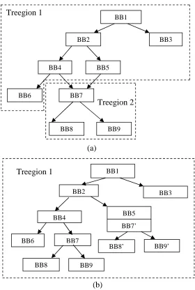
Treegion-based global scheduling aims for high performance for wide issue VLIW / EPIC processors although it can be applied to superscalar processors as well. It has two steps: treegion formation and tree traversal scheduling (TTS). A treegion is a single-entry / multiple-exit nonlinear code region that consists of basic blocks (BBs) with the control-flow forming a tree, as illustrated in Figure 2.1.
Figure 2.1 (a) The CFG and the natural treegion construction; (b) The treegion constructed after tail duplication.
BB1
BB2 BB3
BB4 BB5
BB7
BB9
Treegion 1
Treegion 2
BB6
BB8
BB1
BB2 BB3
BB4 BB5
BB7
BB7’
BB9
Treegion 1
BB8 BB6
BB9’ BB8’
(a)
During tree traversal scheduling (TTS), the BBs in a treegion are scheduled in a predetermined traversal order based on treegion topology and profile information. When a BB is currently being scheduled, those instructions that are dominated by the BB will be considered as scheduling candidates until the block-ending branch is scheduled. In this way, speculation is enabled from all the paths starting from the BB. Those candidate operations are scheduled based on an order determined by a heuristic that includes their execution frequency, exit count, and data dependence height. The details of tree traversal scheduling can be found in [78].
2.3
Profile-Guided Performance Bounds
Due to complexity, many compiler frameworks partition a function body into many multi-path regions and each region is used as a scheduling unit. We establish a lower bound of execution time for such a single-entry multiple-exit region since instructions are rarely moved across the scheduling region boundary. Performing bound computation at the granularity of the scheduling region is important as it captures global instruction scheduling impacts accurately. With region-level performance bounds, we can derive easily the bounds at the procedure/function level and the program level.
Figure 2.2. A CFG example containing three control paths.
f1
f2
f3
For a single-entry multiple-exit region, if execution frequency for each control path is determined from profile information, we can compute the lower bound of execution time (LBET) as a weighted sum of LBET of each path. For the example control flow graph (CFG) shown in Figure 2.2, there are three control paths in the region and the execution frequencies f1, f2, and f3 are associated with each path respectively. So, the lower bound execution time of this region can be computed as the sum of the LBET of each path weighted by its execution frequency. We can write this weighted sum as the following equation.
(
)
∑
∑
= = i path i path i path i path i path i path i path freq bound resource bound dependence data Max freq LBET LBET _ _ _ _ _ _ _ * _ , _ _ * Equation 2-1Resource bound in Equation 2-1 is calculated similar to the ResMII (resource-constrained minimum-initiation-interval) calculation in iterative modulo scheduling [59], as follows.
( _ _ )
_ _ k k
k i
path Max Num Insn Num FU
bound
resource = Equation 2-2
In Equation 2-2, Num_Insnk represents the number of operations that use the
function unit type k. Num_FUk represents the number of function units of type k available
in the processor. The ratio (ceil) of these two numbers shows the resource constraints of function units of type k. Then, resource bound is calculated as the maximum constraint of all types of function units. From our experience, load/store units and branch units are usually critical resources for most integer benchmarks in the SPEC 2000 Integer benchmark suite.
Again, the execution frequency for each path, Freqpath_i, used as the weight of the corresponding path in Equation 2-1, is obtained from edge profiling.
Since the LBET of each scheduling region describes its execution time, the LBET of the whole program is simply the sum of the LBETs of all the scheduling regions. So, we can compute the program-level performance bound with the following steps:
1. Forming the scheduling regions, such as treegions or superblocks, based on the control flow graph.
2. Compute LBET of each region and take the summation as the LBET of the program.
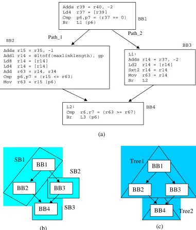
for the same code segment. A code example in IA-64 [32] style assembly is given in Figure 2.3, and the corresponding C code is shown in Figure 2.4.
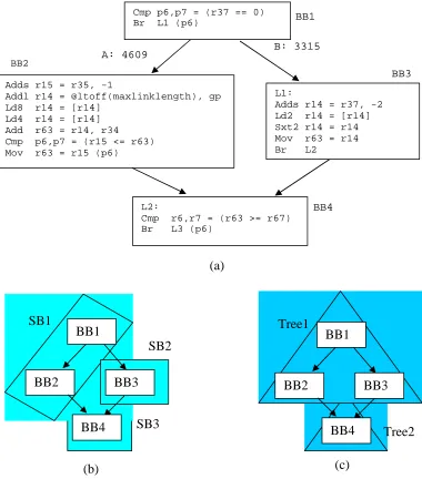
Figure 2.3. (a) Code segment from the benchmark parser (function list_link). Numbers along the edge labels are edge profiles; (b) The superblock formed without
tail duplication; (c) The natural treegion formed.
As shown in Figure 2.3a, the code segment is a simple diamond structure extracted from the benchmark parser. First, we show the bound computation for superblock scheduling. If no code expansion optimization is performed, three superblocks
Cmp p6,p7 = (r37 == 0) Br L1 (p6)
Adds r15 = r35, -1
Addl r14 = @ltoff(maxlinklength), gp Ld8 r14 = [r14]
Ld4 r14 = [r14] Add r63 = r14, r34 Cmp p6,p7 = (r15 <= r63) Mov r63 = r15 (p6)
L1:
Adds r14 = r37, -2 Ld2 r14 = [r14] Sxt2 r14 = r14 Mov r63 = r14 Br L2
L2:
Cmp r6,r7 = (r63 >= r67) Br L3 (p6)
A: 4609 B: 3315
BB2 BB3 BB4 BB1 (a) BB1
BB2 BB3
BB4 SB1 SB2 SB3 (b) BB1
BB2 BB3
BB4 Tree1
Tree2
(SB) are formed for the code segment: SB1 contains BB1 and BB2, SB2 contains BB3, and SB3 contains BB4, as shown in Figure 2.3b. Assuming our machine model has the following configuration: 6-wide issue (2 ALU, 2 ALU/LD/ST, 2 ALU/BR, e.g., Itanium-I and II); load operations have a 2-cycle latency and all other integer operations have a 1-cycle latency (except CMP instructions which can be issued at the same 1-cycle as the consuming branch). We can compute the lower bound of execution time (LBET) of SB1 using Equation 2-1 as: 1*3315 + 8*4609 = 40,187 cycles; LBET of SB2 as 5 * 3315 = 16,575 cycles; and LBET of SB3 as 1 * (3315 + 4609) = 7,924 cycles. The performance bound of the hammock is the sum of the bounds of these superblocks (64,686 cycles).
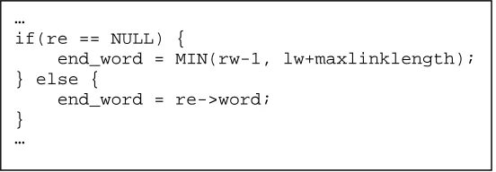
Figure 2.4. The corresponding C code of the assembly code segment in Figure 2.3. The global variable maxlinklength is accessed through a linkage table.
Next, if we use treegions as basic scheduling regions, two natural treegions can be formed for this code example without any code replication: Tree1 contains BB1, BB2, and BB3; and Tree2 contains BB4, as shown in Figure 2.3c. For the same machine model, the LBET of Tree1 is computed as: 4609*8 + 3315*5 = 53,447 cycles; the LBET of Tree2 is 1 * (3315 + 4609) = 7,924 cycles. The LBET of the hammock is the sum of the LBETs of Tree1 and Tree2 (61,371 cycles). Compared to the LBET computed using superblocks, the treegion-based LBET is smaller as it considers the possibility of control speculation not only from BB2 to BB1 but also from BB3 to BB1. The superblock-based
…
if(re == NULL) {
end_word = MIN(rw-1, lw+maxlinklength); } else {
end_word = re->word; }
approach, however, considers speculation only from BB2 to BB1. From this example, it can be seen that the performance bounds also reveal the potential of a particular instruction-scheduling algorithm and it illustrates that treegion scheduling provides better scheduling capabilities by enabling speculation from multiple execution paths.
The region expansion optimization, duplication of BB4 in this example, could potentially reduce the LBET of both superblock-based LBET and treegion-based LBET and this will be discussed in detail in Chapter 3 as we evaluate the performance impact of code size related optimizations.
2.4
Profile Independent Performance Bounds
For real-time applications, the most important objective is to guarantee that a task finishes by a specified deadline instead of reducing the average execution time. As a result, the worst-case execution time (WCET) is commonly used assuming a program will experience its longest control flow path. As our objective is to evaluate WCET reduction of ILP optimizations for real-time applications, we propose a profile-independent bound for a single-entry multiple-exit region as follows:
(
( _ _ , _ ))
_ _ _ _ _ i path i path i path i path i path bound resource bound dependence data Max Max LBET Max LBWT = = Equation 2-3the path with longest execution time) is assumed while the lower bound of execution time is used for each path. Since such a lower bound is used, the actual execution time along the path could potentially exceed this lower bound. So, it apparently conflicts the purpose of worst-case execution time. However, remember that we use LBWT to measure the impact of WCET reduction due to code optimizations instead of using LBWT directly as the final WCET measure. Measuring the actual execution time along each path requires the scheduled code. It is unacceptable in practice since time-consuming instruction scheduling needs to be performed in order to measure the impact for every single code optimization instance. Using LBET for each path, on the other hand, provides an accurate estimate of the actual execution time and associates low computational complexity. Moreover, this LBWT can be used to check the soundness of the deadline setting: if the predetermined deadline exceeds the LBWT, it is impossible that the task can be finished in time when the longest control path is taken. In such a case, the system has to reassign the deadlines, adopt a more powerful processor, or optimize the code more aggressively.
Computing LBWT at the function level is complicated due to complex CFGs and multiple regions in a function body. Although we can use a simple approach, such as taking the summation of the LBWTs of each region as the LBWT for the function, the computed bounds are overly pessimistic as many impossible control paths are assumed.
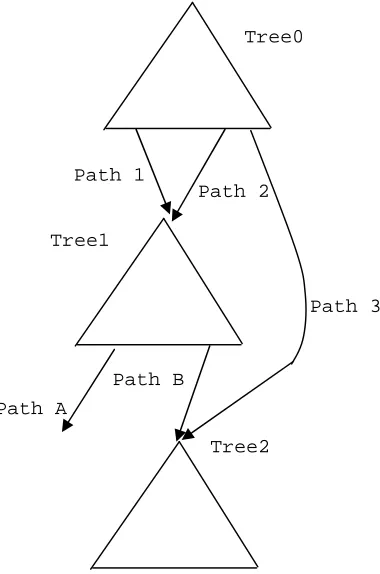
effect accurately, especially the control speculation effect, and limits the enumeration of the possible control paths. Next, we use an example to derive this treegion-based LBWT analysis. We start with an innermost loop body, which may contain more than one treegion. One such example is shown in Figure 2.5.
Figure 2.5. Deriving LBWT in a complex CFG without loops.
The CFG in Figure 2.5 contains three treegions. In order to compute the LBWT of such a code segment, we extend Equation 2-3 to Equation 2-4 to compute the LBWT for each treegion. The LBWT for treegion 0 in this example is the LBWT for the overall code segment.
LBWT = Max(LBETpath_1+LBWTbase_path_1, …, LBETpath_k+LBWTbase_path_k)
Equation 2-4
Path A
Path B
Tree2 Tree1
Tree0
Path 1
Path 2
In Equation 2-4, LBWT of a treegion is computed as the maximum LBWT of every path in the treegion, which is in turn defined as the sum of the LBET of the path (LBETpath_i) and the LBWT of the treegion that the path leads to (LBWTbase_path_i). The
term LBETpath_i is defined as before, i.e., the maximum of the data dependence bound and
the resource bound. The term LBWTbase_path_i is computed recursively using Equation 2-4
based on the control dependence relationship among treegions. For exit paths or return paths, LBWTbase is zero. For the code example in Figure 2.5, the overall LBWT (i.e.,
LBWT of treegion 0) is computed as follows:
LBWTtreegion0 = Max(LBETpath_1+LBWTbase_path_1, …, LBETpath_k+LBWTbase_path_k)
= Max(LBETpath_1+LBWTtreegion1, LBETpath_2+LBWTtreegion1, LBETpath_3+LBWTtreegion2).
LBWTs of treegion 1 and treegion 2 can be computed in turn as:
LBWTtreegion1 = Max(LBETpath_A, LBETpath_B+LBWTtreegion2);
LBWTtreegion2 = Max(LBETpaths_in_treegion2).
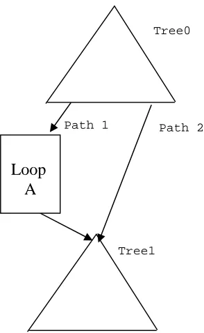
For an outer loop body or a CFG containing loop structures, such as the CFG shown in Figure 2.6, the LBWT can be computed as follows,
LBWTtreegion0 = Max(LBETpath_1+LBWTloop_A, LBETpath_2+LBWTtreegion1).
where LBWT of loop A is computed as LBWTloop_body_A * loop_count_A + LBWTtreegion1.
LBWT for the loop body (LBWTloop_body_A) can be computed using Equation 2-4 if it
contains more than one treegion and the loop count is determined from the workload specification or from profiling.
Figure 2.6. A CFG containing a loop structure.
As a final note, if we replace the LBET along each path with the actual schedule length/execution time, the LBWT becomes the WCET.
Next, we use a code example to illustrate the LBWT computation. The code example is a simple diamond structure as shown in Figure 2.7. Here, we use it to illustrate the LBWT computation and also show that treegion-based scheduling will result in a smaller LBWT compared to superblock scheduling or trace scheduling, making treegion scheduling more suitable for real-time applications.
First, we compute the superblock-based LBWT using the same 6-issue machine model as used in Section 2.3. The LBWT of the code segment is the same as LBWTSB1,
which is computed as follows using Equation 2-4:
LBWTSB1 = Max(LBETpath_1+LBWTSB3, LBETpath_2+LBWTSB2)
= Max(LBETpath_1+LBWTSB3, LBETpath_2+ LBETSB2_path +LBWTSB3)
= Max(8 + 1, 4 + 5 + 1) = 10 cycles. Tree1
Tree0
Path 1 Path 2
From this computation, it seems that control path 2 forms the critical path.
Figure 2.7. (a) The similar code example to Figure 2.3; (b) The superblocks formed without tail duplciation; (c) The natural treegion formed.
Using treegions as basic scheduling regions, the LBWT of the code segment is
LBWTtree1, which is computed as follows using Equation 2-4:
Adds r39 = r40, -2 Ld4 r37 = [r39]
Cmp p6,p7 = (r37 == 0) Br L1 (p6)
Adds r15 = r35, -1
Addl r14 = @ltoff(maxlinklength), gp Ld8 r14 = [r14]
Ld4 r14 = [r14] Add r63 = r14, r34 Cmp p6,p7 = (r15 <= r63) Mov r63 = r15 (p6)
L1:
Adds r14 = r37, -2 Ld2 r14 = [r14] Sxt2 r14 = r14 Mov r63 = r14 Br L2
L2:
Cmp r6,r7 = (r63 >= r67) Br L3 (p6)
Path_1 Path_2
BB2 BB3 BB4 BB1 (a) BB1
BB2 BB3
BB4 SB1 SB2 SB3 (b) BB1
BB2 BB3
BB4 Tree1
Tree2
LBWTtree1 = Max(LBETpath_1+LBWTtree2, LBETpath_2+LBWTtree2)
= Max(8 + 1, 5 + 1) = 9 cycles.
Chapter 3
Compiling for Code Size
Efficiency
In this chapter, we describe how we use our proposed profile-guided performance bounds to guide code compilation for code size efficiency. The objective is to selectively perform ILP optimizations so that significant ILP improvement is achieved at a very small cost in static code size increase. A brief background on ILP optimizations is contained in Section 3.1. Section 3.2 presents performance bound driven code size efficiency. Section 3.3 contains our proposed algorithm to regulate code size related ILP optimizations. The optimal tradeoff between performance improvement and code size is defined in Section 3.4, and a simple heuristic is developed to achieve this optimum. Section 3.5 contains the experimental methodology and results. A summary of this chapter is provided in Section 3.6.
3.1
Background on Code Size Related ILP Optimizations
related optimizations for integer workloads, we focus on the three most commonly used ILP optimizations: tail duplication, loop unrolling and if-conversion.
Tail duplication (or code replication) replicates a subgraph of the control flow to remove side entries of a trace [6],[31] and to avoid conditional / unconditional branches [56]. Many instruction-scheduling approaches [28],[31],[51] use tail duplication in forming scheduling regions. Due to its evident impact on static code size increase, different heuristics have been proposed to decide whether a particular instance of tail duplication should be performed. One simple example is a threshold on the profiled execution frequency [31]. However, there is no systematic way to analyze the tradeoff between the cost in code size and the performance gain.
If-conversion [2],[58] replaces conditional branches with appropriate predicate computations, and the instructions that are control dependent on the branch are guarded with these predicates. The removal of frequently mispredicted branches can yield large performance gains [50]. Also, if-conversion increases the spatial locality of instructions and may reduce code size if the targeted instruction set architecture (ISA) uses predicate computation for a conditional branch, such as IA-64 [32],[65] or HPL-PD [35]. As pointed out in [4], full if-conversion generally works for compiling numerical applications. For integer applications, selective if-conversion [4] is essential to achieve performance gains due to the potential hazards of if-conversion [15]. Hyperblock formation involves a complex heuristic to choose which paths to be included and then performs conversion on the selected basic blocks [51]. Profile based selective conversion [55] uses profile information to compute the performance gain of if-conversion based on weighted schedule estimates before and after predicating a hammock. The schedule estimates are based on local scheduling results. Compared to this estimate, our performance bound calculation is more accurate as it considers the potential effects pf speculation on each scheduling region.
3.2
Performance Bound Driven Code Size Efficiency
In this section, we first define the notion of code size efficiency (CSEF). Then, we use tail duplication, loop unrolling, and if-conversion to explain how to use performance bounds to calculate this efficiency.
3.2.1
Code size efficiency
The major objective of code size related optimizations is to improve instruction level parallelism (ILP). One direct measure of the effectiveness of such a transformation is the ratio of ILP improvement over the code size increase. Since code optimizations are performed at compile time, we use static instructions-per-cycle (IPC) to measure ILP improvement. The static IPC is computed as the ratio of the number of retired instructions (IC) over execution time (ET). Both IC and ET are derived from profile information. The speculated instructions resulting from instruction scheduling are not included in IC. Using the ratio of ILP improvement over code size increase as a quantitative measure (as stated, such a measure is intuitively appealing and we will show later in Section 3.4 that it is indeed a good measure), two formal definitions of code size efficiency for code transformations are proposed.
First, we define the efficiency for an instance of a code transformation, called the
n applicatio individual before n applicatio individual after n applicatio individual before n applicatio individual after inst size code size code IPC IPC Efficiency _ _ _ _ _ _ _ _ . _ _ − − = Equation 3-1
In Equation 3-1, the term in the numerator represents the ILP improvement of a particular instance of a code optimization, and the term in the denominator represents the cost of such an optimization in terms of static code size. Using loop unrolling as an example, if we unroll a particular loop once, the instantaneous efficiency of such an unrolling is the performance gain divided by the size of the loop body. Since there could be many loops in a program, there is one such instantaneous efficiency associated with each of them.
The definition in Equation 3-1 measures the performance impact at the cost of unit code size increase for a single instance of a code transformation. It is also useful to have a quantitative measure when more than one optimization instance has been performed. For example, assume a program has three loops. One unroll heuristic picks all three of them to be unrolled once and another heuristic may unroll just one loop many times. A quantitative measure would be able to tell which heuristic performs better in balancing performance and code size. Such a measure is what we define as average code size efficiency, shown in Equation 3-2.
original candidate original candidate average size code size code IPC IPC Efficiency _ _ − −
= Equation 3-2
average efficiency can be viewed as averaging the instantaneous efficiencies of each individual code optimization that has been performed.
Note that the IPC improvement in Equations 3-1 and 3-2 closely correlates to the execution time reduction. In fact, we may use the ratio of execution time reduction over code size change to approximate code size efficiency (the difference between this ratio and the formal efficiency definition is a near constant factor for a given program). This ratio is easy to understand and intuitively appealing as it basically tells how many cycles can be saved at the cost of one additional instruction.
3.2.2
Using performance bounds to calculate code size efficiency
Equation 3-3
3.2.3
Examples of code size efficiency computation
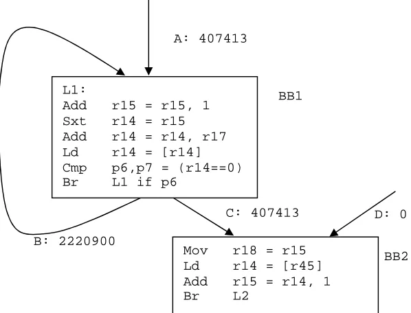
First, we focus on code transformations resulting in ILP improvement as well as code size increase. Both tail duplication and loop unrolling are such optimizations. Using a code segment from the benchmark twolf as an example, shown in Figure 3.1, we explain how to compute the code size efficiency.
The code segment shown in Figure 3.1 has two basic blocks (BB1 and BB2), a loop back edge (edge B), and a merge point (edges C and D), exhibiting the possibility of applying both loop unrolling and tail duplication.
Figure 3.1. A code segment from twolf (in function new_dbox_a). Numbers along control edge labels are edge profiles.
L1:
Add r15 = r15, 1 Sxt r14 = r15 Add r14 = r14, r17 Ld r14 = [r14] Cmp p6,p7 = (r14==0) Br L1 if p6
Mov r18 = r15 Ld r14 = [r45] Add r15 = r14, 1
Br L2
A: 407413
C: 407413 D: 0
Assuming load instructions have a 2-cycle latency and all other instructions in BB1 and BB2 have a 1-cycle latency (except CMP instructions which can be scheduled at the same cycle as the consuming branch), the lower bound execution time (LBET) before any transformation is the sum of the LBET of BB1 and the LBET of BB2. Assuming a 6-wide issue (2 ALU, 2 ALU/LD/ST, 2 ALU/BR) machine (which causes no resource constraints in this example), the LBET can be computed using Equation 2-1: LBET of BB1 is 6*2,628,313 = 15,769,878 cycles, LBET of BB2 is 3*407,413 = 1,222,239 cycles, and the sum is 16,992,117 cycles. After duplicating BB2, the instructions in BB2 can be scheduled in BB1 using control speculation, which results in an LBET of 15,769,878 cycles as the inclusion of BB2 instructions does not increase the true data dependence height (i.e., an LBET reduction of 1,222,239 cycles due to complete hiding of BB2 execution time). Therefore, the instantaneous code size efficiency of tail duplication occurring at the merge point of edges C and D is 1,222,239 / 4 = 305,560 cycle/instruction, i.e., one additional instruction leads to a 305,560 cycle execution time reduction.
As shown in Figure 3.2, the probability propagation maintains the taken/not taken probability of the conditional branches at the end of BB1 and BB1’ (the unrolled copy of BB1). After the profile is redistributed, the LBET of the loop body in Figure 3.2 (containing BB1 and BB1’) can be computed using Equation 2-1 (9,751,148 cycles). Compared to the LBET of the loop body with no unrolling, LBET reduction is 15,769,878 – 9,751,148 = 6,018,730 cycles. Therefore, the instantaneous code size efficiency of loop unrolling (with factor 1) at back edge B is: 6,018,730 / 6 = 1,003,121 cycles/instruction.
Figure 3.2. Loop unrolling of the loop body shown in Figure 3.1 with unroll factor of 2. (Numbers along control edge labels are edge profiles computed using probability
propagation.)
If-conversion can reduce code size by removing branch instructions. Also, it may result in positive speedups by removing branch misprediction penalties. Therefore, the code size efficiency can be a negative number (i.e., positive speedup and negative code size increase), which represents one highly desired extreme of code size efficiency. (The other extreme of negative speedup and positive code size increase is what we always
BB1
BB1’
BB2
A: 407413
D: 0 C1: 220821
C2: 186592 B1: 1203746
want to avoid.) Using another simple code segment from the benchmark twolf, we show how we compute the efficiency of if-conversion by integrating branch misprediction penalties. The code segment is shown in Figure 3.3.
Using Equation 2-1, the LBET of the region containing BB1, BB2 and BB3 is computed as 28,111*2+169,174*3 = 563,744 cycles. Then, we consider potential branch misprediction penalties. Assuming static branch prediction and a 10-cycle misprediction penalty for each misprediction, the overall misprediction penalty of the conditional branch in BB1 is 28,111*10 = 281,110 cycles. If the profile of dynamic branch prediction is available, more accurate penalty computation can be used.
Figure 3.3. A code segment from twolf (function add_penal) to show efficiency of if-conversion. Numbers along control edge labels are edge profiles.
After if-conversion, the branches in BB1 and BB3 are removed (i.e., 2-instruction reduction) and the resulting LBET is 3*(28,111+169,174) = 591,855 cycles, which means a reduction of (563,744+281,110-591,855) = 252,999 cycles. Note that this computation involves only the control dependent blocks of the conditional branch (BB1, BB2 and
Cmp p6,p7 = (r36 != r18) Br L1 (p6)
Ld r14 = [r16] Ld r15 = [r20]
L1:
Ld r14 = [r34] Sub r14 = r33, r14 Ld r15 = [r16] Br L2
L2:
Add r14 = r14, r15 …
A: 28111 B: 169174
BB2
BB3
BB3). It does not depend on the merge block (BB4), and the same result holds when BB4 has more than 2 entry edges.
As pointed out previously, optimizations with positive speedups and negative code size increase are always performed. So, we do not need to calculate the actual efficiency for such cases. For if-conversions that have both negative speedup and negative code size increase, positive code size efficiency results. Such efficiency implies that we may want to perform if-conversion with low positive efficiency to reduce code size (although hurting performance slightly) and use the saved code size for optimizations with higher efficiency.
3.3
Regulating Code Size Related ILP Optimizations
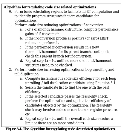
Based on the quantitative measure of code size efficiency defined in Section 3.2, we develop an algorithm to regulate code size related optimizations, as shown in Figure 3.4.
Figure 3.4. The algorithm for regulating code size related optimizations.
Optimizations are treated differently based on their code size efficiency characteristics. Optimizations with positive speedup and negative code size increase are examined first in Step 1 of the algorithm. Then, an iterative approach is used to selectively perform code-expanding optimizations, as shown in Step 2 of the algorithm. First, step 2a computes the efficiency of all potential optimization instances. Then, the best candidate is found from these instances based on their efficiency in step 2b. Next, if the one with the best efficiency passes the feasibility check, it will be performed in step
Algorithm for regulating code size related optimizations
0. Form basic scheduling regions to facilitate LBET computation and
to identify program structures that are candidates for optimizations.
1. Perform code size reducing optimizations: if-conversion
a. For a diamond/hammock structure, compute performance
gains of if-conversion.
b. If the if-conversion produces positive (or zero) LBET
reduction, perform it.
c. If the performed if-conversion results in a new
diamond/hammock for its parent branch, continue to check this parent branch for if-conversion.
d. Repeat step 1a – 1c, until no more diamond/hammock
structures need to be checked.
2. Perform code size increasing optimizations: loop unrolling and
tail duplication
a. Compute instantaneous code size efficiency for each loop
unrolling / tail duplication candidate using Equation 3-1.
b. Search the candidate list to find the one with the best
efficiency.
c. If the selected candidate passes the feasibility check,
perform the optimization and update the efficiency of candidates affected by the optimization. The feasibility check may involve code size constraints, register pressure, etc..
d. Repeat step 2a – 2c, until the overall code size reaches a
2c. The feasibility check basically makes sure that a particular optimization will not result in excessive resource utilization, e.g., the size of a loop body is less than the level one I-cache size. As one particular optimization may change the efficiency of another optimization or enable another optimization (e.g., a tail duplication may enable a diamond/hammock to be constructed for if-conversion), a local efficiency update is performed in Step 2c if one optimization instance is performed. Note that this iterative approach can automatically choose a good unroll factor for a loop by unrolling the original loop body one iteration at a time.
3.4
Optimal Tradeoff between ILP Improvement and Code
Size Increase
Figure 3.5. An example curve showing the relationship of ILP improvement and code size increase.
Figure 3.5 shows an example ILP vs. code size curve, which exhibits common characteristics of individual benchmarks we studied (see Section 3.5.3). The diminishing returns are due to the rapidly decreasing code size efficiencies, which in turn is due to the following two fundamental reasons. First, based on the definition of code size efficiency, an instance optimization with high efficiency should have high execution frequency. The well-known ‘90/10 rule’ points out that a small part of the static code (hot portions) consumes most of the execution time. After performing optimizations in these hot portions of code, the remaining optimizations should have much lower efficiencies due to the much lower execution frequency. Secondly, high efficiency also requires that the resulting code must have better performance bounds, i.e., the instance optimization must reduce the DDG height without causing any resource conflict problems. This requirement filters the optimizations applied in hot portions of a program.
The diminishing returns phenomenon shown in Figure 3.5 enables us to define the optimal tradeoff between ILP improvement and code size increase. One natural choice is
Relative code size Static
IPC
100%
High efficiency range
the ‘knee’ of the curve in Figure 3.5, provided that the corresponding code size still satisfies the overall feasibility check.
To automatically find this knee in the curve, a simple heuristic is developed by taking advantage of the steep slope of the high efficiency part of the ILP vs. code size curve, as shown in Figure 3.6. Figure 3.6 replicates the ILP vs. code size curve in Figure 3.5 and the knee of the curve is marked as point A.
Figure 3.6. Achieving the optimal tradeoff between ILP improvement and code size increase.
To locate A, we can first use two straight lines to approximate the curve (as the dashed lines L1 and L2 shown in Figure 3.6). Then, the knee of the curve becomes the
intersection, A’, of these two lines. A simple threshold scheme can be used to find A’: the point along the curve whose slope is between the slope of L1 and the slope of L2. The
slope of the ILP vs. code size curve represents the ratio of static IPC changes over relative code size changes, which is exactly the definition of the instantaneous code size efficiency in Equation 1. So, the approach to achieve the optimum tradeoff is simply as follows: perform the optimizations whose instantaneous code size efficiency is higher than the threshold efficiency K. This threshold efficiency can be any value between the slope of L1 and the slope of L2. In other words, the range between the slope of L1 and
Relative code size Static
IPC
A
L1
slope of L2 determines the robustness of this threshold scheme. In our experiments (see
Section 3.5.4), we vary K from tan(π/12) (corresponding to a line with an angle of 15 degrees) to tan(π/6) (corresponding to a line with an angle of 30 degrees) to show the robustness of this threshold scheme. This threshold K is both workload-independent and
input-independent.
As we use the ratio of LBET change over absolute code size increase (measured in number of instructions) to compute code size efficiency, we can further derive the threshold scheme as in Equation 3-4. The derivation details can be found in Appendix A.
static static
absolute
IPC
IC
LBET
K
dSize
LBET
d
∗
∗
≥
−
)
(
Equation 3-4
In Equation 3-4, ICstatic represents the static operation count of the program (i.e.,
the static program size; whereas the term ICdynamic is the number of retired instructions
during execution and is used for IPC calculation), K is the threshold on instantaneous code size efficiency, LBET is the lower bound of execution time for the whole program,
d(-LBET) is the reduction in the lower bound (both are computed using Equation 2-1), and IPCstatic (= LBET / ICdynamic ) represents the ILP feature of the original program.
3.5
Experimental Results
3.5.1
Methodology
In our experiments, we use the SPEC CINT 2000 benchmarks [30] to evaluate the proposed algorithms. The benchmarks are first compiled into IA-64 assembly using the
gcc compiler (version 3.1). As our purpose is to regulate ILP optimizations, we use the level one optimization provided by gcc to perform classical optimizations (as discussed in Section 3.5.2, a by-product of the level one optimization is that gcc produces predicated code). The resulting IA-64 assembly codes are then parsed into the LEGO compiler framework [41], which we use to implement the algorithms in this chapter. The IA-64 assembly is instrumented and executed to gather profile information. In our experiments, we use the reference input data set and skip the first 500 million instructions and profile the next 500 million instructions for each benchmark.
In Table 3.1, we also include the ratio of estimated execution time of treegion-scheduled code over the lower bound. The execution time of treegion-treegion-scheduled code is computed using a scoreboard dependency-enforcing approach (i.e., it is the execution time assuming ideal caches and ideal branch prediction). From these results, it can be seen that the treegion scheduler produces quite a good schedule, exceeding 1% to 13% of the lower bound. The mismatch is because the performance bound is calculated assuming that all false register dependencies can be removed by software renaming, and that control dependencies can be minimized by multiway branch transformations. Such assumptions are too optimistic as liveness beyond the basic block scope may require a copy instruction to be inserted. Resource conflicts due to speculation from multiple paths in a treegion are another reason.
Table 3.1. Baseline results including static code size, execution time, and static IPC.
Baseline bzip crafty gap gzip mcf parser twolf vortex Vpr
Static size (num
of insn.) 7543 51085 131447 13316 2548 25545 65786 120735 35416
Number of dynamic insn.
Retired 498M 490M 500M 495M 491M 496M 496M 499M 497M
Lower bound of
exe. time (cycles) 257M 217M 495M 275M 276M 263M 325M 219M 318M
Static IPC 1.93 2.26 1.01 1.80 1.78 1.87 1.53 2.27 1.56
Ratio of natural tree schedule results over the
lower bound 104% 108% 104% 112% 106% 113% 107% 107% 101%
3.5.2
Regulating code size decreasing optimizations – if-conversion
prediction to estimate branch misprediction penalties assuming that each misprediction incurs a 10-cycle penalty.
Table 3.2 shows the if-conversion results using our algorithm. As stated previously, the input IA-64 assembly code is generated using the GNU gcc compiler with level one optimizations, which perform not only classical optimizations but also if-conversion. By applying our algorithm to this already if-converted code, we show that our algorithm can improve upon gcc’s if-conversion algorithm.
Table 3.2. If-conversion results.
bzip2 crafty gap gzip mcf parser twolf vortex vpr If-conversions
(by gcc) 113 780 2852 139 61 502 1042 1692 325 Number of
conditional br. 487 2712 9747 819 167 2068 3625 7469 1805 If-conversion
with pos. gain 2 40 1 6 5 2 11 4 10
If-conversion
with zero gain 19 163 324 26 7 80 445 191 74 If-conversion
with neg. gain 4 58 2 3 4 1 24 37 8
No if-conversion:
complex CFG 358 1608 5752 546 133 1483 2787 2161 1263 No
if-conversion:
ret_call 104 843 3668 238 18 502 358 5076 450 Number of
dynamic cond.
br. 36.4M 23.8M 23.6M 37.4M 71.0M 46.0M 33.8M 32.8M 30.5M Reduction in
execution time including br. misprediction penalty
(cycles) 91016 1057363 9700 799877 90688 80125 506372 122592 13148695 static br.
misprediction
Interesting observations can be made from Table 3.2. The first row in Table 3.2 reveals that gcc has removed a significant amount of conditional branches through predication, although the second row, which shows the number of existing conditional branches in each benchmark after gcc’s if-conversion, suggests that there still exist potential if-conversion candidates. Our algorithm examines those conditional branches and confirms that the majority of these conditional branches are hard to if-convert. We report those hard-to-convert conditional branches in two categories: row 6 shows the number of conditional branches followed by a complex CFG (e.g., merging points at both if path and else path of a diamond/hammock) inhibiting diamond/hammock detection, and row 7 presents the number of detected diamonds/hammocks containing function call, return, or indirect branch instructions. (We excluded the case where both paths contain the same function call or return instruction) In such cases, if-conversion may hurt branch prediction performance as it may introduce more conditional function calls and returns, which in turn incur branch misprediction penalties. For those if-convertible branches, our algorithm computes the performance gain. Using the benchmark gzip as an example, gcc
converts 139 conditional branches and there remain 819 conditional branches in the program. Our algorithm finds that 546 of them do not form a diamond/hammock structure. For those that form a diamond/hammock, 238 of them have at least a function call or a return along one or both paths. For the remaining ones, 6, 26, and 3 of them produce positive, zero, and negative speedups, respectively.
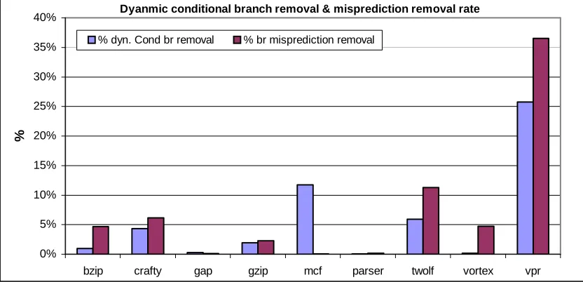
number of these if-conversion instances seems limited (1 to 40), significant performance gains can be achieved, as shown in Figure 3.7.
Dyanmic conditional branch removal & misprediction removal rate
0% 5% 10% 15% 20% 25% 30% 35% 40%
bzip crafty gap gzip mcf parser twolf vortex vpr
%
% dyn. Cond br removal % br misprediction removal
Figure 3.7. The removal rate of dynamic conditional branches and mispredictions by if-conversion.
Finally, we analyze the code size reduction impact of if-conversion. We choose to perform if-conversion instances with positive or zero gains in this experiment. Assuming each conversion saves two instructions in IA-64 assembly, the overall code size reduction is computed and is shown in Figure 3.8. Remember that this reduction is achieved on the IA-64 code that has already been predicated by gcc. This demonstrates that our algorithm reduces code size by performing if-conversion more aggressively. From Figure 3.8, it can be seen that if-conversion reduces static code size consistently for every benchmark, up to 1.4% (the benchmark twolf) and 0.68% on average. Although these numbers seem to be trivial, in the next subsection, we will show that utilizing such a small amount of code size can lead to very large ILP improvements.
Static code reduction by if-conversion
0.00% 0.20% 0.40% 0.60% 0.80% 1.00% 1.20% 1.40% 1.60%
bzip crafty gap gzip mcf parser twolf vortex vpr ave.
%
3.5.3
Results of regulating code size increasing optimizations – tail
duplication and loop unrolling
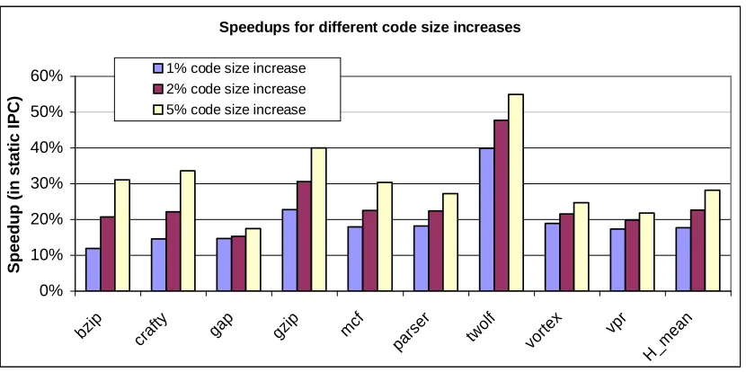
Step 2 of the algorithm shown in Figure 3.4 regulates code size increasing optimizations (tail duplications and loop unrolling). It iteratively selects and performs the one instance of tail duplication or loop unrolling with the highest instantaneous efficiency. In this experiment, we examine the effectiveness of such an iterative approach. For each benchmark, we set the limit of overall code size increase at 1%, 2%, and 5% of its original size (i.e., the optimization stops when the overall code size reaches this limit). The corresponding ILP improvements are shown in Figure 3.9.
Speedups for different code size increases
0% 10% 20% 30% 40% 50% 60%
bzip crafty gap gzip mcf pars er twol f vorte x vpr H_m ean S p e e d u p ( in s ta ti c I P C )
1% code size increase 2% code size increase 5% code size increase
Figure 3.9. The speedups for different code size increases.
size saved by aggressively performing code-reducing transformations can be used for code expanding optimizations with high efficiency. This is the reason that the algorithm in Figure 3.4 performs code-reducing transformations before code enlarging ones. Secondly, it can be seen from Figure 3.9 that further code-size increase has less impact on ILP improvement. As shown in the figure, an additional speedup of 5% on average is observed as the code size increases from 1% to 2% of its original size, still significant but less impressive compared to 18% for the first 1% of code size increase. The reason is that during the iterative selection process, the efficiency of the selected optimization decreases rapidly. Using the benchmark vortex as an example, the first selected optimization is one tail-duplication in procedure Chunk_ChkGetChunk with an efficiency as high as 534,609 cycles/instruction. After another 7 optimizations were selected and performed (resulting in replicating 66 instructions), the efficiency of the next chosen optimization drops to 77,484 cycles/instruction. As discussed in Section 3.4, two main reasons account for such ‘diminishing returns’: the ‘90/10’ rule and the reduction in data dependence height without causing resource conflicts.
ILP improvement vs. code size increase (mcf)
1.5 1.7 1.9 2.1 2.3 2.5 2.7
0% 10% 20% 30% 40% 50% 60%
relative code size increase
s
ta
ti
c
I
P
C
(a)
ILP improvement vs. code size increase (twolf)
1 1.2 1.4 1.6 1.8 2 2.2 2.4 2.6
0% 10% 20% 30% 40% 50% 60%
relative code size increase
s
ta
ti
c
I
P
C
(b)
Figure 3.10. ILP improvement vs. code size increase for benchmarks (a) mcf and (b)
twolf.