Graphical Models for Structured Classification, with an Application to
Interpreting Images of Protein Subcellular Location Patterns
Shann-Ching Chen [email protected]
Department of Biomedical Engineering Carnegie Mellon University
Pittsburgh, PA 15213, USA
Geoffrey J. Gordon [email protected]
Machine Learning Department Carnegie Mellon University Pittsburgh, PA 15213, USA
Robert F. Murphy [email protected]
Departments of Biological Sciences, Biomedical Engineering, and Machine Learning Carnegie Mellon University
Pittsburgh, PA 15213, USA
Editor: Nir Friedman
Abstract
In structured classification problems, there is a direct conflict between expressive models and ef-ficient inference: while graphical models such as Markov random fields or factor graphs can rep-resent arbitrary dependences among instance labels, the cost of inference via belief propagation in these models grows rapidly as the graph structure becomes more complicated. One important source of complexity in belief propagation is the need to marginalize large factors to compute mes-sages. This operation takes time exponential in the number of variables in the factor, and can limit the expressiveness of the models we can use. In this paper, we study a new class of potential functions, which we call decomposable k-way potentials, and provide efficient algorithms for com-puting messages from these potentials during belief propagation. We believe these new potentials provide a good balance between expressive power and efficient inference in practical structured classification problems. We discuss three instances of decomposable potentials: the associative Markov network potential, the nested junction tree, and a new type of potential which we call the voting potential. We use these potentials to classify images of protein subcellular location patterns in groups of cells. Classifying subcellular location patterns can help us answer many important questions in computational biology, including questions about how various treatments affect the synthesis and behavior of proteins and networks of proteins within a cell. Our new representation and algorithm lead to substantial improvements in both inference speed and classification accuracy.
Keywords: factor graphs, approximate inference algorithms, structured classification, protein subcellular location patterns, location proteomics
1. Introduction
example, if each instance is a handwritten character, the side information might be that the string of characters forms a common English word; or, if each instance is a microscope image of a cell with a certain protein tagged, the side information might be that several cells share the same tagged protein. To solve such a structured classification problem in practice, we need both an expressive way to represent our beliefs about the structure, as well as an efficient probabilistic inference algorithm for classifying new groups of instances.
Unfortunately, the goal of having an expressive language is in direct conflict with the goal of having an efficient inference algorithm: while Markov random fields or factor graphs can represent arbitrary dependences among instances, inference rapidly becomes intractable as the graph structure becomes more complicated (see, e.g., Koller and Friedman, 2007). Simple graphs such as pairwise links arranged in chains or trees lead to efficient inference, but these structures may not allow us to express our beliefs accurately or completely. On the other hand, if we try to couple large groups of labels (either directly, by specifying a factor that links to a large number of labels, or indirectly, by using a graph with large loops), the cost of inference grows exponentially.
To speed up inference, we can move to approximate algorithms such as loopy belief propagation (see, e.g., Koller and Friedman, 2007). Loopy belief propagation handles large loops efficiently, but it does nothing to speed up the task of working with single large factors. In fact, in practical problems, the operation of marginalizing a large factor can easily become the main bottleneck for inference, preventing us from using more-expressive models.
Therefore, in this paper, we study a new class of potential functions, which we call decom-posable k-way potentials. Computing messages for these potentials is much more efficient than for general potentials, even though the new potentials can express distributions that cannot be rep-resented by groups of smaller potentials. Accordingly, we believe these new potentials provide a better balance between expressive power and efficient inference than was previously available.
We discuss three instances of decomposable potentials: the associative Markov network poten-tial, the nested junction tree, and a new type of potential which we call the voting potential. We use these potentials to classify images of protein subcellular location patterns in groups of cells. Classifying protein subcellular location patterns is important as a step in solving many practical computational biology problems, particularly in the area of systems biology: for example, it can help in designing high-throughput screening systems for drug discovery, or in conducting experi-ments to determine the effect of various treatexperi-ments on the synthesis and behavior of proteins and networks of proteins within a cell. Our new representation and algorithm lead to substantial im-provements in both inference speed and classification accuracy.
Preliminary versions of portions of this work have been presented previously (Chen and Mur-phy, 2006; Chen et al., 2006a,b). These papers describe applications of decomposable potentials and the corresponding fast inference algorithms for segmenting and classifying images of protein subcellular location patterns. But, none of these papers describe the idea of decomposable potentials of Section 4 or the nested inference algorithm of Section 5 in full generality. They also do not cover some of the instances of decomposable potentials described in Section 6; and, the experiments of Sections 8–9 have not been reported previously.
2. Factor Graphs
f
1f
3f
2x
1x
2x
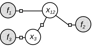
3Figure 1: A probability distribution represented as a factor graph. Small squares denote potential functions; for example, this factor graph contains a potential which connects the variables x1, x2, and x3, and another which connects x1and f1.
on only a subset of the variables, and the overall probability distribution is the product of the local factors, together with a normalizing constant Z:
P(x) = 1
Zfactors j
∏
ϕj(xV(j)).Here V(j)is the set of variables that are arguments to factor j; for example, ifϕjdepends on x1, x3,
and x4, then V(j) ={1,3,4}and xV(j)= (x1,x3,x4).
Each variable xior factorϕjcorresponds to a node in the factor graph. Fig. 1 shows an example:
the large nodes represent variables, with shaded circles for observed variables and open circles for unobserved ones. The small square nodes represent factors, and there is an edge between a variable xi and a factor ϕj if and only if ϕj depends on xi, that is, when i∈V(j). (By convention the
graph only shows factors with two or more arguments. Factors with just a single argument are not explicitly represented, but are implicitly allowed to be present at each variable node.)
The inference task in a factor graph is to combine the evidence from all of the factors to compute properties of the distribution over x represented by the graph. Naively, we can do inference by enumerating all possible values of x, multiplying together all of the factors, and summing to compute the normalizing constant. Unfortunately, the total number of terms in the sum is exponential in the number of random variables in the graph. So, usually, a better way to perform inference is via a message-passing algorithm called belief propagation (BP). Here we briefly review the basics of BP in factor graphs; for more details, see Kschischang et al. (2001).
The basic BP algorithm works on a factor graph which is tree-shaped (i.e., has no cycles). It sends messages from every variable to each of its neighboring factors, and from every factor to each of its neighboring variables. Messages to or from a variable xiwill be vectors whose length is equal
to the number of values that xican take on.
For a variable xi with neighboring factorsϕ1,ϕ2, . . . ,ϕk, suppose that x has received messages mj→i(xi) from its neighborsϕj for j∈ {1. . .(k−1)}. (To simplify notation, we have numbered
xi’s neighbors consecutively starting from 1. This is not a loss of generality since we can always
temporarily permute our factor indices to make it so.) Suppose also that xi has local evidence
represented by the one-argument factorϕloci (xi). Then we can compute xi’s message toϕkas
mi→k(xi) =ϕloci (xi)
k−1
∏
j=1
That is, we take the componentwise product of all of the messages from factors 1. . .k−1, multiply in the local evidence, and send the result toϕk. The normalization of the message is arbitrary, so for convenience or numerical precision we may multiply each component of the message by an arbitrary constant.
Similarly, suppose that a factorϕj has neighbors x1,x2, . . . ,xk (again numbered consecutively
without loss of generality) and has received messages mi→j(xi)for i∈ {1. . .(k−1)}. Then we can computeϕj’s message to xkas
mj→k(xk) =
∑
x1
∑
x2
. . .
∑
xk−1
ϕj(x1, . . . ,xk)
k−1
∏
i=1
mi→j(xi). (2)
Unlike Equation 1, in Equation 2 we must marginalize out variables other than xkby summing over
their possible values.
BP works by picking an arbitrary node of the graph as root and then making two passes over the tree: first it passes messages inward from the leaves to the root, and then outward from the root to the leaves. When the message passing finishes, the posterior marginal probability of any random variable xiis just the componentwise product of its local potential and all of its incoming messages:
P(xi) =ϕloc(xi)
∏
{j|i∈V(j)}
mj→i(xi). (3)
2.1 Working with General Graphs
The above discussion assumed that our factor graph was tree-shaped. For graphs with loops, we have two alternatives: first, we can collapse groups of variable nodes together into combined nodes, which can turn our graph into a tree and allow us to run BP as above. Second, we can run an approximate inference algorithm that doesn’t require a tree-shaped graph. We can also combine these alternatives if desired, grouping variable nodes to reduce the number of loops in the graph so that our approximate inference becomes more accurate.
When we combine a set of variable nodes, the new node represents all possible settings of all of the original nodes. E.g., if we collapse a variable x1that has settings T,F with a variable x2that has settings A,B,C, then the combined variable x12has settings TA,T B,TC,FA,FB,FC. When we collapse a set of variables, we need to alter the neighboring factor nodes: any factor adjacent to any of the original nodes becomes a neighbor of the new combined node, and its list of arguments is extended if necessary to include all variables in the collapsed set.
The advantage of collapsing variable nodes is that it can allow us to simplify the structure of our graph: if in the collapsed graph there are two factor nodes with the same set of arguments, then we can combine them by multiplying their potentials elementwise. For example, Fig. 2 shows the result of collapsing x1 and x2 in the factor graph of Fig. 1. The potentialsϕ23 andϕ123 from the original graph have the same set of neighbors in the new graph, and so can be combined into one factor node. Similarly, the local potentialsϕloc1 andϕloc2 can be combined with the factorϕ12to form a new local potential at the collapsed node x12. Notice that the new factor graph is tree-shaped, even though the original one had loops.
f
1f
3f
2x
12x
3Figure 2: Another factor graph that can represent the same probability distribution as the graph of Fig. 1. The new graph was derived by collapsing together the nodes for variables x1and x2from Fig. 1.
x
1x
2x
5x
3x
4x
1x
23x
24x
5Figure 3: A factor graph with multiple loops (left) and a tree derived from the factor graph by collapsing pairs of nodes (right).
disagree, at least one potential must be zero. The cost of storing or working with such a hard-constraint potential depends only on the number of distinct variables in its argument list.
For example, in the graph of Fig. 3, we could form a tree by collapsing x2, x3, and x4 into a single node. The resulting graph would have variables x1, x234, and x5, and factorsϕ1234andϕ2345. But, we can form a tree with smaller factors if we group x2with x3and also separately with x4: the resulting graph has variables x1, x23, x24, and x5, and factorsϕ123,ϕ234, andϕ245. The potentialϕ234 encodes the constraint that the settings of x23and x24must agree on the assignment to x2.
A factor graph that has been reduced to a tree is equivalent to a junction tree. A junction tree is a connected acyclic graph whose nodes are labeled with sets of variables in a way that satisfies the running intersection property: if a variable is present at two nodes A and B, it is also present at all nodes along the (unique) path connecting A and B in the tree. The factor nodes in a tree-shaped factor graph correspond to nodes of the junction tree, with labels equal to their argument sets. The collapsed variable nodes correspond to edges of the junction tree. The groups of original variables at each collapsed variable node (such as{x2,x4}in the figure) are called separators, since conditioning on all of the variables in a separator is sufficient to separate the factor graph into two or more disconnected pieces. The running intersection property ensures that we can define potentials that constrain all copies of a variable to agree.
for message calculation (Equations 1–2). However, we may have to update each message several times before the marginals converge. The version of the algorithm that updates messages repeatedly until convergence is called loopy BP, or LBP. Inference with LBP is approximate because it can double-count evidence: messages to a node i from two nodes j and k can both contain information from a common neighbor l of j and k. Several researchers have empirically demonstrated that when LBP converges, the posterior marginal probabilities from Equation 3 often approximate the true marginals well (Murphy et al., 1999; McEliece et al., 1998; Zhang and Chang, 2004). If LBP oscil-lates between some steady states and does not converge, we can stop the process after some number of iterations; in this case, the approximate posteriors will usually be inaccurate. Although oscilla-tions can be avoided by using “momentum” (Murphy et al., 1999), which replaces the messages that were sent at time t with a weighted average of the messages at times t and t−1, in some cases the approximate posteriors are still inaccurate (Murphy et al., 1999). The convergence of LBP depends on the exact graph structure and on the type and strength of the factors involved (Pearl, 1988; Hes-kes, 2004). Recently, researchers have developed sufficient conditions for the convergence of LBP (Weiss, 2000; Tatikonda and Jordan, 2002; Ihler et al., 2005), and a measurement of message errors has been proposed (Ihler et al., 2005).
For either exact or loopy BP, the runtime for each pass over the factor graph is exponential in the number of distinct original variables included in the largest factor. So, inference can become prohibitively expensive if our factors are too large, either because they were too large in the original graph or because we merged too many variables.
3. Factor Graphs and Structured Classification
To use belief propagation to solve structured classification problems, we need two things: a local classifier for individual instances, and a factor graph which encodes our prior beliefs about likely arrangements of instance labels. The local classifier tells us the likelihood of individual test exam-ples under each possible class assignment, while the factor graph tells us how to trade off evidence at one example against evidence at another. We can learn local classifiers in a number of ways; for the cell image classification experiments below, we use standard support vector machines, together with a post-processing step that allows us to interpret the SVM outputs as probabilities.
3.1 The Potts Potential
The simplest potential function is the Potts potential. The Potts potential is a pairwise (i.e., two-argument) factor which encourages two nodes xiand xjto have the same label:
ϕ(xi,xj) =
ω
xi=xj
1 otherwise. (4)
Hereω>1 is an arbitrary parameter which expresses how strongly we believe that xiand xjhave the
same label. If we use one Potts potential for each edge in the similarity graph, the overall probability of a vector of labels x is
P(x) = 1
Znodes i
∏
P(xi)edges i∏
,jϕ(xi,xj) (5) where we have written Z for a normalizing constant and P(xi) for the probability which the base classifier assigns to label xifor node i. Equations 4–5 form what is known as a Potts model.Unfortunately, the Potts model does not perfectly capture our desired intuition about inference from labels of neighboring cells. To see why, consider a two-class prediction problem where node xi
has kAneighbors of class A and kBneighbors of class B, and suppose that classes A and B have equal
prior probability for xigiven the classifier output. In this situation the ratio of posterior probabilities
for classes A and B will beωkA−kB. So for example, ifωis 2, and if x
ihas 1 neighbor of class A and
3 of class B, then the ratio of probabilities will be 21−3=1/4. So, class A will be 1/4 as likely as class B, and P(xi has label A) =0.2.
However, if xihas 7 neighbors of class A and 9 neighbors of class B, the posterior probability of
class A will still be 0.2, even though our intuition tells us that the probability should be much closer to 0.5 in this case. The same will hold whenever there are 2 more neighbors of class B than class A, even if the counts are 107 and 109. Worse, as class B’s majority gets larger, the ratio of probabilities will approach 0 exponentially fast. So, a sufficiently strong vote from xi’s neighbors will quickly
overwhelm any evidence at xiitself—an undesirable situation.
The source of this problem is that, in Equation 5, the evidence from separate potentials has to combine multiplicatively. So, as long as the evidence from different neighbors acts through separate potentials, we will see an exponential dependence between the number of neighbors of a given class and the probability of that class. We can reduce the severity of this problem by choosingωto be only a little bit larger than 1. But, to fix the problem we need to move to potential functions that depend on k>2 nodes. Our experimental results, below, will show that potentials that combine evidence additively can perform better than the Potts potential over a wider range of inference problems.
3.2 The Voting Potential
To capture the intuition that we should be less certain about nodes whose neighbors split relatively evenly, we propose a new potential which we call the voting potential. In the voting potential, a node’s classification is influenced by the proportion of classes among its neighbors, rather than the difference in class counts as in the Potts model.
x1 x2 x3 ϕ
0 0 0 3/4
0 0 1 1/2
0 1 0 1/2
0 1 1 1/4
1 0 0 1/4
1 0 1 1/2
1 1 0 1/2
1 1 1 3/4
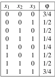
Table 1: An example of the voting potential with parameterλ=2 for n=2 classes. The center node x1has two neighbors, x2and x3.
We define the voting potential as follows:
ϕj(xV(j)) =
λ/n+∑i∈N(j)I(xi,xj)
|N(j)|+λ . (6)
Here n is the number of classes,λis a smoothing parameter, and I is an indicator function:
I(xi,xj) =
1 if xi=xj
0 otherwise.
(The normalization constant in the denominator of Equation 6 is irrelevant to inference, and is included only for ease of interpretation.) An example of the voting potential is given in Table 1.
The voting potential function combines the evidence from all of node xj’s neighbors into a
summary vote which then influences x’s classification. The parameterλcontrols how much weight we put on a vote from a small number of neighboring cells. We can interpret it as the size of an additional set of fictitious neighbors whose votes are distributed uniformly; this trick limits the influence of a vote from a small number of neighbors, and is called Laplace smoothing. For example, looking at the first and fifth rows of the table, we can see that when both of x1’s neighbors are 0, x1 is 3 times as likely to be 0 as 1, since there are 2+1 votes for x1=0 and 0+1 votes for x1=1.
The behavior of the voting potential contrasts with that of the Potts potential described in Sec-tion 3.1, in which each neighbor separately influences the center node without reference to the other neighbors. In line with our intuition, we will see below that networks which use the voting potential can yield more accurate results than the Potts model for structured classification problems.
3.3 The AMN Potential
The associative Markov network (AMN) potential (Taskar et al., 2004) is defined to be
ϕ(x1. . .xk) =1+ n
∑
y=1
(ωy−1)I(x1=x2=. . .=xk=y) (7)
for parametersωy>1, where I(predicate)is defined to be 1 if the predicate is true and 0 if it is false. So, the AMN potential is constant unless all of the variables x1. . .xk are assigned to the same class
The AMN potential reduces to the Potts potential when k=2 and ωy=ω for all y. So, in this case it inherits the same problems that the Potts potential has. For any k, the AMN potential has no direct effect on a label vector’s likelihood unless all of the k argument variables agree on the label y. (It affects all vectors’ likelihoods indirectly through the normalizing constant.) As k gets larger, there are comparatively fewer label vectors where all k labels agree, and so the AMN potential may not have much influence on the overall posterior distribution over label vectors unless the cell-level classifiers already were very close to agreement. And in fact, our experiments below demonstrate that factor graphs based on the AMN potential perform best when the neighborhood size k is relatively small (but larger than 2).
4. Decomposable Potentials
While k-way factors can lead to more accurate inference, they can also slow down belief propaga-tion. For a general k-way factor, it takes time exponential in k even to look at all of the entries. So, we cannot expect to find inference algorithms for general k-way potentials that take less than exponential time.
For specific k-way potentials, though, we can hope to take advantage of special structure to de-sign a fast inference algorithm. In particular, for many interesting potential functions, we can write down an algorithm which efficiently performs sums of the form required for message computation:
∑
x1
∑
x2
. . .
∑
xk−1
ϕ∗
j(x1, . . . ,xk), (8) ϕ∗
j(x1, . . . ,xk) =m1(x1)m2(x2). . .mk(xk−1)ϕj(x1, . . . ,xk). (9)
Here mi(xi)is the message to factor j from variable xi. (If we removed loops in our factor graph by
collapsing groups of variables, then Equation 9 may look instead like
ϕ∗
j(x1, . . . ,xk) =m12(x1,x2)m245(x2,x4,x5). . .mk−1(xk−1)ϕj(x1, . . . ,xk).
That is, the argument sets of the messages may overlap with one another. The derivations below apply equally well to either expression forϕ∗j.)
For example, as we will see below, we can compute Equations 8–9 quickly if ϕj is a sum of
terms ∑lψjl where each term ψjl depends only on a small subset of its arguments x1. . .xk. Or,
we can compute Equations 8–9 quickly ifϕj is constant except at a small number of input vectors (x1, . . . ,xk). In the first case we will say thatϕj is a sum of low-arity termsψjl, and in the second
case we will say thatϕj is sparse.
More generally, suppose thatϕ∗j in Equation 8 can be written as a sum of products of low-arity functions: writingψjlfor a generic term in the sum andξjlmfor a generic factor ofψjl,
ϕ∗
j(x1, . . . ,xk) =
Lj
∑
l=1
ψjl(x1, . . . ,xk) =
Lj
∑
l=1
Mjl
∏
m=1
ξjlm(xV(j,l,m)) (10)
where the set of indices V(j,l,m)⊆ {1. . .k}tells us which variablesξjlmdepends on. Also suppose
that, for each termψjl in the sum, the sets V(j,l,m)can be arranged into a junction tree. That is,
suppose that we can build a cycle-free graph on Mjl nodes, with one node labeled with V(j,l,m)
Ifϕ∗j satisfies the above properties, and if Lj, Mjl, and|V(j,l,m)|are small for all j, l, and m,
then we will say that ϕ∗j is decomposable. And, we will say thatϕj is a decomposable potential
(in the context of this message computation). Decomposable potentials include the special cases mentioned above, namely sparse potentials and potentials that are sums of low-arity terms, as well as a wide variety of other examples which we will describe in more detail below. We will see below that we can evaluate Equations 8–9 quickly for a decomposable potential by using an algorithm very similar to belief propagation.
5. Belief Propagation with Decomposable Potentials
When we are running BP or loopy BP on a factor graph with decomposable potentials, we can accelerate the computation of the belief messages that would otherwise be slow to compute. There are two types of messages that we need for BP or loopy BP, shown in Equations 1 and 2.
Messages from a variable (or a separator, which we treat as a single large variable) to a factor are fast to compute in any case: we can calculate them from Equation 1 by looping over the incoming edges at node xiand, for each edge, looping over the n possible classes we can assign to xi. So, we
do not need to accelerate the computation of these messages.
Messages from a factor to a variable (Equation 2) are slow to compute na¨ıvely if the factor connects to many other variables. In this section we will show that we can calculate these messages efficiently for decomposable potentials of the form shown in Equation 10. So, this section shows that we can implement BP and loopy BP efficiently for decomposable potentials. The derivation of this section works with general decomposable potentials; below, in Sections 6.1 and 6.2, we will work out the formulas for specific cases including the voting potential and the associative Markov network potential.
The algorithm that we will use to compute the messages is essentially the same as the overall belief propagation algorithm. So, when we perform inference on a factor graph with decomposable potentials, we will be running two nested copies of belief propagation: the inner copy will act on a single decomposable potential, and will compute the messages which the outer copy needs to send from that potential.
Substituting Equations 8–10 into Equation 2 and rearranging terms tells us that the desired message is
mj→k(xk) =
∑
x1
∑
x2. . .
∑
xk−1
ϕj(x1, . . . ,xk)
k−1
∏
i=1
mi→j(xi)
=
∑
x1
∑
x2
. . .
∑
xk−1
Lj
∑
l=1
Mjl
∏
m=1
ξjlm(xV(j,l,m))
!
=
Lj
∑
l=1
∑
x1∑
x2. . .
∑
xk−1
Mjl
∏
m=1
ξjlm(xV(j,l,m)). (11)
Now let us fix l temporarily, leaving a term of the form
∑
x1
∑
x2
. . .
∑
xk−1
Mjl
∏
m=1
We have assumed that the sets V(j,l,m)for m∈ {1, . . . ,Mjl}can be arranged into a junction tree.
Pick a node of this junction tree whose label contains xk, and call this node the root. Refer to each
node by its index m, and write par(m)for the parent of node m.
Now pick an arbitrary leaf of the junction tree. Without loss of generality, say that this leaf has index m=1. We can partition the variables in the set V(j,l,1)into two subsets,
C(1) =V(j,l,1)∩V(j,l,par(1)) and D(1) =V(j,l,1)\V(j,l,par(1)).
C(1) contains the variables that node 1 has in Common with its parent, while D(1) contains the variables from node 1 that are Distinct from its parent’s variables. The variables in D(1)can only appear in V(j,l,1): if any of them appeared in V(j,l,m) for m6=1 it would violate the running intersection property, since any path from 1 to m has to pass through par(1).
Without loss of generality, suppose that the variables in D(1)are numbered consecutively from 1, say D(1) ={1,2}. That means that the factorξjl1depends on x1and x2, but no other factorξjlm
for m6=1 depends on x1or x2. So, by the distributive law, we can rearrange Equation 12 as follows:
∑
x3
. . .
∑
xk−1
Mjl
∏
m=2
ξjlm(xV(j,l,m)).
∑
x1
∑
x2
ξjl1(xV(j,l,1))
!
(13)
To get Equation 13 we have moved the x1and x2summations inward as far as possible.
We can think of the expression in parentheses in Equation 13 as a message which travels from node 1 to node par(1)of the junction tree: it depends only on the variables in the set C(1), and it summarizes everything that node par(1)needs to know about node 1 in order to compute the term of Equation 12. We will write µ1→par(1)for this message, that is,
µ1→par(1)(xC(1)) =
∑
x1
∑
x2
ξjl1(xV(j,l,1)). (14)
We can continue computing messages in this fashion from leaf nodes of the junction tree to their parents. After several steps our expression will look something like this:
∑
x7
. . .
∑
xk−1
Mjl
∏
m=4
ξjlm(xV(j,l,m))
3
∏
m=1
µm→par(m)(xC(m)). (15)
Here we have eliminated the variables x1through x6 and computed the messages from nodes m=
1,2,3 to their parents. At this point suppose that node m=4 is an internal node of the junction tree, and that it has as its only child node m=1. Because we have already computed the message from node 1 to node 4, we can now compute the message from 4 to par(4). Suppose that D(4) ={7}; then we can rearrange Equation 15 as follows.
∑
x8
. . .
∑
xk−1
Mjl
∏
m=5
ξjlm(xV(j,l,m))×
3
∏
m=2
µm→par(m)(xC(m))
∑
x7
µ1→4(xC(1))ξjl4(xV(j,l,4))
!
. (16)
intersection property, 7 would have to be an element of V(par(4))and couldn’t be in D(4). The message µ1→4could depend on x7, since 7 could be in C(1). So, to be safe, we have left µ1→4inside the x7summation. On the other hand, the messages µ2→par(2)and µ3→par(3)cannot depend on x7: if one of them did, 7 would have to be in V(j,l,par(2))or V(j,l,par(3)), which would again violate the running intersection property.
In a natural generalization of Equation 14, we will write µ4→par(4)(xC(4)) for the expression in parentheses in Equation 16. It should be clear at this point that we can compute a message from each node in the junction tree to its parent, so long as we work from the leaves upward; the message from a node m to its parent par(m)will depend on the messages from m’s children to m. Once we process all of the children of the root r, we will be left with an expression that contains summations only over variables in V(j,l,r). (In fact, it will contain summations over exactly the variables in V(j,l,r)\ {k}.) We can perform these summations to find the desired term (Equation 12), which is a function only of xk. We can then repeat the process for each l to get all of the terms in Equation 11.
The above algorithm computes the message from a factorϕjto a single neighboring variable xk.
If we want the messages fromϕjto all of its variables we can run the above algorithm multiple times;
however, the multiple runs will redundantly recompute many of the messages µs→t. Instead, as is
usual for the belief propagation algorithm, we can combine all of the runs into a single computation which passes one message in each direction over each edge of the junction tree.
If we have merged groups of variables in constructing our outer junction tree, then there are two modifications needed for the above analysis. First, if the argument sets of the incoming messages at a given factor node overlap, we may need to build different inner junction trees to compute different outgoing messages. So, we may not be able to share computation as described in the previous paragraph. This loss of sharing may increase our runtime by a small factor. Second, and more importantly, if the desired outer message depends on several original variables, then there may be no node of our inner junction tree that contains all the needed variables. In this case we may condition on the possible values of some of the needed variables, and use several runs of inner message passing, each of which computes a slice of the desired outer message. In general, there may be several ways to decompose a potential, and several possible choices of which variables to condition on for a given decomposition. Each of these setups may lead to a different runtime for message computation. See Section 6.3 below and Kjærulff (1998) for more details.
6. Instances of Decomposable Potentials
Decomposable potentials are common and useful. In this section, we discuss the details and deriva-tions of message passing with the voting potential, the associative Markov network potential, and the nested junction tree.
6.1 Decomposing the Voting Potential
The general BP-style algorithm of Section 5 is more complicated than we need when we are com-puting messages for the voting potential: since Equation 6 is a sum of low-arity functions rather than a sum of products of low-arity functions, the computation for each term in the sum is particularly simple. So, in this section we will derive efficient expressions for the necessary messages.
There are two types of messages we need to think about: those from a factorϕj to the node
xk thatϕj is centered on, and those from a factor ϕj to some non-centered variable node xi with
messages mi→j(xi)so that∑ximi→j(xi) =1. With these assumptions, the message from a factorϕj
to its center variable node xkcan be computed as follows:
(λ+|N(j)|)mj→k(xk)
=
∑
x1
∑
x2
. . .
∑
xk−1
λ/n+
k−1
∑
i=1
I(xi,xk)
!
k−1
∏
i0=1
mi0→j(xi0)
= λ
n
∑
x1∑
x2 . . .x∑
k−1
k−1
∏
i0=1
mi0→j(xi0) +
∑
x1
∑
x2
. . .
∑
xk−1
k−1
∑
i=1
I(xi,xk)
k−1
∏
i0=1
mi0→j(xi0)
= λ
n+
k−1
∑
i=1
∑
x1∑
x2
. . .
∑
xk−1
I(xi,xk)
k−1
∏
i0=1
mi0→j(xi0)
= λ
n+
k−1
∑
i=1
∑
x1∑
x2
. . .
∑
xk−1
I(xi,xk)mi→j(xi)
k−1
∏
i0=1,i06=i
mi0→j(xi0)
= λ
n+
k−1
∑
i=1
∑
xiI(xi,xk)mi→j(xi)
= λ
n+
k−1
∑
i=1
mi→j(xk).
The first equation above is the definition of the desired message. The second equation distributes multiplication over addition. The third equation uses the fact that all terms in the product
∏k−1
i0=1mi0→j(xi0)are independent, along with our assumption∑x
i0mi0→j(xi0) =1, to compute the first
summation. The fourth equation factors mi→j out of the product. The fifth equation uses again the
facts that all terms in the product are independent and∑x
i0mi0→j(xi0) =1. The last line uses the fact
that I(xi,xk)is nonzero iff xi=xk.
The message from a factor j to a non-centered variable can be computed similarly. Under the same assumptions as above, we will calculate the message mj→1:
(λ+|N(j)|)mj→1(x1)
=
∑
x2
. . .
∑
xk
λ/n+
k−1
∑
i=1
I(xi,xk)
!
k
∏
i0=2
mi0→j(xi0)
= λ
n+
∑
x2
. . .
∑
xk
k−1
∑
i=1
I(xi,xk) k
∏
i0=2
mi0→j(xi0)
= λ
n+
∑
x2
. . .
∑
xk
I(x1,xk)
k
∏
i0=2
mi0→j(xi0) +
∑
x2
. . .
∑
xk
k−1
∑
i=2
I(xi,xk) k
∏
i0=2
mi0→j(xi0)
= λ
n+
∑
xk
I(x1,xk)mk→j(xk) +
∑
x2
. . .
∑
xk
k−1
∑
i=2
I(xi,xk) k
∏
i0=2
mi0→j(xi0)
= λ
n+mk→j(x1) +
∑
x2 . . .∑
xk
k−1
∑
i=2
I(xi,xk) k
∏
i0=2
= λ
n+mk→j(x1) +
k−1
∑
i=2
∑
x2. . .
∑
xk
I(xi,xk)mi→j(xi)mk→j(xk)
k−1
∏
i0=2,i06=i
mi0→j(xi0)
= λ
n+mk→j(x1) +
k−1
∑
i=2
∑
xi∑
xk
I(xi,xk)mi→j(xi)mk→j(xk)
= λ
n+mk→j(x1) +
k−1
∑
i=2
∑
xkmi→j(xk)mk→j(xk).
The first equality above is the definition of the desired message. The second pulls the term λ/n out of the sums, using the facts that the terms in the product ∏ki0=2mi0→j(xi0)are independent and
∑xi0mi0→j(xi0) =1. The third equality splits the sum over i into two pieces, one for i=1 and the
other for i≥2. The fourth equality uses the independence of the terms in the left-hand product to simplify away the summations over x2through xk−1. The fifth uses the fact that I(x1,xk) =0 when
x16=xk. The sixth equality pulls the terms mi→jand mk→jout of the remaining product. The seventh
uses the independence of terms in the product to simplify away the summations over variables other than xiand xk. And the last equality uses the fact that I(xi,xk) =0 when xi6=xk.
Despite the fact that the variables x1, . . . ,xk have exponentially many possible assignments, the
above derivations show that we can compute the messages mj→k and mj→1 exactly and almost instantaneously. The message mj→k is particularly easy to interpret: it is the (Laplace smoothed)
average of the messages from x1, . . . ,xk−1. 6.2 Decomposing the AMN Potential
It is even easier to derive an efficient expression for the messages from an AMN potential than it was for the messages from a voting potential. As before, let us assume that V(j) ={1, . . . ,k}, that we desire the message mj→k(xk), and that we have normalized the messages mi→j(xi) to sum to 1
over xi for each i=1, . . . ,k−1. Since the AMN potential is symmetric in its arguments, there is
only one type of message to calculate.
We can write Equation 7 in the form of Equation 10 by noting that
I(x1=x2=. . .=xk=y) =I(x1=y)I(x2=y). . .I(xk=y)
and that each function I(xi=y) depends on only one variable xi. Given this representation, the
desired message is:
mj→k(xk) =
∑
x1
∑
x2
. . .
∑
xk−1
1+
∑
y(ωy−1) k
∏
i=1
I(xi,y)
!
k−1
∏
i0=1
mi0→j(xi0)
= 1+
∑
x1
∑
x2. . .
∑
xk−1
∑
y
(ωy−1) k
∏
i=1
I(xi,y)
k−1
∏
i0=1
mi0→j(xi0)
= 1+
∑
y(ωy−1)I(xk,y)
∑
x1
∑
x2
. . .
∑
xk−1
k−1
∏
i=1
I(xi,y)mi→j(xi)
= 1+
∑
y(ωy−1)I(xk,y)
k−1
∏
i=1
mi→j(y)
= 1+ (ωxk−1)
k−1
∏
i=1
The first equality above is the definition of the desired message. The second pulls the constant 1 outside of the sums and uses the independence of terms in the product. The third rearranges the order of the sums and products. The fourth uses the fact that the product is zero unless xi=y for all
i∈ {1, . . . ,k−1}. The fifth uses the fact that I(xk,y)is 0 unless xk=y.
6.3 The Nested Junction Tree
The nested junction tree method (Kjærulff, 1998) can speed up message propagation in the junction trees that arise when we remove loops from a factor graph. In particular, it helps compute messages from the large factors that arise when we merge groups of variables. It works by noticing that each of these messages is computed from the product of many smaller factors, which can sometimes be arranged into a nontrivial “inner” junction tree.
Unlike the previous two examples (the voting and AMN potentials), the nested junction tree method does not attempt to look inside the factors of the original factor graph. Instead, it keeps track of the variable merges during junction tree construction, and sometimes is able to “undo” some of these merges temporarily to provide computational savings.
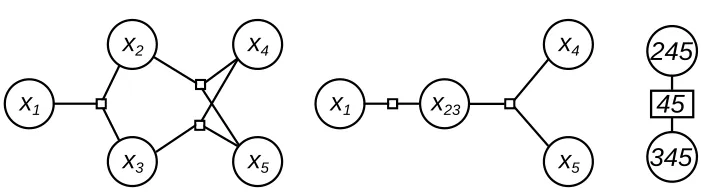
For example, the factor graph of Fig. 4 can be collapsed into a junction tree by merging x2and x3as shown. The time and space costs of belief propagation on this junction tree are dominated by its largest potential,ϕ2345. Consider the message fromϕ2345to x23:
m2345→23(x2,x3) =
∑
x4
∑
x5
ϕ2345(x2,x3,x4,x5)m4→2345(x4)m5→2345(x5).
Standard belief propagation will first compute
ϕ∗
2345(x2,x3,x4,x5) = ϕ2345(x2,x3,x4,x5)m4→2345(x4)m5→2345(x5)
= ϕ245(x2,x4,x5)ϕ345(x3,x4,x5)m4→2345(x4)m5→2345(x5) for all settings of(x2,x3,x4,x5), and then marginalizeϕ∗2345to get m2345→23.
If there are (for example) ten possible settings of each original variable, the space required for computing m2345→23 with standard belief propagation is 10100 locations: 104 for storingϕ∗2345, and 102 for storing m2345→23. And, the time cost is 39900 flops: for each of the 104 settings of
(x2,x3,x4,x5)we must multiply together one element each from the tablesϕ245,ϕ345, m4→2345, and m5→2345, at a cost of 3 flops per iteration. Then, for each of the 102elements of m2345→23, we must sum 102elements ofϕ∗2345(using 102−1 flops), leading to a total cost of 3×10000+99×100.
However, if we examine the message computations in more detail, it turns out that we can take advantage of the structure ofϕ∗2345 to save time and space. Sinceϕ∗2345was formed by multiplying together four smaller tables, and since the argument sets of these smaller tables form a junction tree,
ϕ∗
2345is decomposable. (The inner junction tree is shown at the far right of Fig. 4.) Using this fact, we can find m2345→23 by passing messages through the inner junction tree several times. In more detail, suppose we pick the factorϕ345 as the root of the inner junction tree. This factor contains one of the message variables (x3) but not the other one (x2). So, we must condition on each value of x2in turn. For each value of x2, we first compute the intermediate message
ϕx2(x
x
1x
2x
4x
3x
5x
1x
23x
4x
5245
45
345
Figure 4: A factor graph for which the nested junction tree method can speed up belief propagation. Left: original factor graph. Middle: factor graph after merging x2 and x3. Right: inner junction tree for computing the message m2345→23.
This message is associated with the separator{x4,x5}in the inner junction tree. We can then incor-porate this inner message into the factor{x3,x4,x5}, and marginalize to get a slice of our desired (outer) message:
m2345→23(x2,x3) =
∑
x4
∑
x5
ϕ345(x3,x4,x5)ϕx2(x4,x5).
Each pass through the inner junction tree keeps x2 fixed, computing a slice m2345→23(x2,·)of the outer message. (By m2345→23(x2,·), we mean a table of the values of m2345→23 for a fixed value of the first argument and all possible values of the second argument.)
The nested belief propagation algorithm for computing m2345→23saves us both space and time. For time, the cost to compute an element of one of theϕx2 tables is 2 multiplications; there are
102 elements of each table, and 10 tables, so the total cost of this step is 2×10×100=2000 flops. To computeϕ345(x3,x4,x5)ϕx2(x4,x5)for fixed x2 takes 1000 flops (one per table element), and to marginalize out (x4,x5) takes 99 flops for each of the 10 resulting elements, for a total of 1000+10×99=1990 per slice. Since there are 10 slices, we need 19900 flops for all of them. The grand total is therefore 19900+2000=21900, a savings of approximately 45% compared to standard belief propagation.
The space savings are even greater: we can reuse a single array of size 102 for all of theϕx2
tables, and a single array of size 103 for all of the productsϕ345(x3,x4,x5)ϕx2(x4,x5). Adding in the cost of storing the final message, we have a space cost of 100+1000+100=1200 locations, a savings of about 88%.
An important limitation of the nested junction tree method is the following lemma, which pro-vides a lower bound on inference time based on the number of variables in the largest node label (or clique):
Lemma 1 In a junction tree T with binary variables, let C be the largest clique, and say that we
wish to compute the posterior marginal for some variable xq. So long as C is minimal, the nested
junction tree method cannot reduce the time for this inference task to less thanΩ(2|C|). (The time for non-binary variables is at least as large.)
Proof Each edge(i,j)in clique C arises either because there is a potential that directly links vari-ables xiand xj (this case includes so-called “moral edges”), or because we triangulated a chordless
cycle that contains xi and xj (in which case some other clique sends C a message that links xi with
these edges when computing outgoing messages from C: for a message M from C to some other clique D, we can ignore the corresponding incoming message N from D to C. Without N, we may be able to ignore as many as |M2|of the edges of C while calculating M, since each edge that connects two variables in M may be supported only by N.
Because we can ignore some of the edges of C, we can avoid building a single large table of size 2|C|, and instead run a nested copy of the message passing algorithm to find M. This inner message passing algorithm works on an inner junction tree T0built from the remaining edges of C. To compute M, we pick some clique C0of T0as root; then, for each possible setting of the variables in M\C0, we pass messages from leaves to root in T0to find a slice of M. This slice corresponds to the fixed setting of M\C0, and covers all possible settings of the variables in M∩C0.
To calculate the total cost of these inner runs of message passing, we need to look at the structure of T0. In particular, we need to figure out the size of the largest clique of T0. For this purpose, we can divide the variables of T0into three sets: those in M\C0(which we hold fixed during each inner iteration), those in M∩C0(which form the resulting slice of M), and those in C\M (the rest of C). The variables in M∩C0are fully connected to one another, since they are all members of C0. And, the variables in C\M are fully connected to one another, since none of them are covered by the incoming message N. But, these two sets of variables are also fully connected to each another: no edge between C\M and M∩C0can be covered by N, since each such edge has one vertex in M and one outside of M. So, C\M and M∩C0together form a clique of T0.
Recapping, we have 2|M\C0|inner runs of message passing, each of which works with a junction tree containing a clique of size|C\M|+|M∩C0|. We will now prove by induction that inference takes time at least k2|C|, where k is an implementation-dependent constant.
For the inductive step, our runtime for calculating M is at least
2|M\C0|×k2|C\M|+|M∩C0|
for 2|M\C0|runs of message passing, each of which costs k2|C\M|+|M∩C0|by the inductive hypothesis. Since|M\C0|+|C\M|+|M∩C0|=|C|, our runtime is therefore at least k2|C|, as claimed.
There are several possible base cases. The most obvious is when |C|=1; in this case we can choose k>0 so that the runtime is at least 2k. The induction can also bottom out if the nested junc-tion tree method becomes inapplicable at any step. There are two ways it can become inapplicable: first, if M\C0= /0, then the argument above means that the nested junction tree has only a single clique of size|C|, and the nested junction tree method therefore offers no speedup. In this case we need to build a table of size 2|C|for inference. So, we can again choose k>0 so that our runtime is at least k2|C|.
Second, the nested junction tree method is inapplicable if clique C has no outgoing messages. C has no outgoing messages if and only if we select it as the root for message passing. In this case, C gets incoming messages from all of its neighbors, and the nested junction tree method again offers no speedup: to perform any inference task on C’s fully-connected graph, we must again build a table of size 2|C| and take time at least k2|C|for some k>0.
So, by choosing k>0 small enough to satisfy all of the above base cases, we have completed the induction. The only remaining detail is the question of non-binary variables. But, it should be obvious from the proof above that any non-binary variables can only increase the cost of inference.
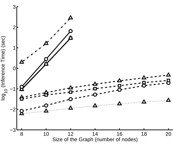
to work with trees with very large cliques. This conclusion is borne out by the experimental results of Kjærulff (1998), Tables 1 and 2: the time savings shown there are never greater than about 60%. In contrast, the examples of the previous two sections show that decomposable potentials in general can lead to far greater savings: in these examples, the message calculation time goes from exponential to polynomial in the size of the clique, and Fig. 10 below shows that this change can easily result in speedups of multiple orders of magnitude.
7. Prior Updating
By calculating messages as described in Section 6.1, we can run loopy belief propagation on a factor graph that includes voting potentials. However, we might expect the messages from a factorϕj to
a non-centered variable xi (where i6=cj) to be fairly weak: the overall vote of all of xcj’s neighbors
will not be influenced very much by xi’s single vote, so there will not be a strong penalty if xivotes
the wrong way.
This observation suggests an even simpler algorithm for inference: we can run loopy BP but ignore all of the messages from factors to non-centered variables. (Ignoring a message means considering it to be uniform.) We will call this algorithm Prior Updating, or PU, since it works by using the current classifications of a node’s neighbors to update the prior for the node’s own classification. Our group proposed a version of Prior Updating for inference on graphs (Chen and Murphy, 2006) before the work described in the current paper, which explores its relationship to potential functions in loopy belief propagation.
We can expect that PU will be noticeably faster than loopy BP, since there will usually be many more non-centered variables than there are centered ones in each factor. We might also hope that PU could be more accurate than loopy BP, since it is less prone to double-count evidence: we have broken any loops which would allow a message that xcj sends to factorϕj to return back and
influence the classification of xcj. (As it turns out, we will see below that in our experiments PU
is often slightly worse and sometimes slightly better than loopy BP on factor graphs with voting potentials.) We will examine the speed and classification performance of loopy BP, PU, and other inference methods in Section 9. PU can be seen as an approximation of LBP on factor graphs with voting potentials, and like LBP, is not guaranteed to converge. However, in our experiments, we never observed problems with convergence for PU or for LBP with the voting potential.
8. Experimental Materials and Methods
2D HeLa Image Set We applied our methods to the problem of classifying subcellular patterns in an image of many cells, a problem that we have formalized previously (Chen and Murphy, 2006). The starting point is a set of fluorescence microscope images of HeLa cells created by introduc-ing antibodies and molecular probes against proteins in major subcellular organelles (Boland and Murphy, 2001). The data set contains 862 single-cell images from ten classes, with each class hav-ing between 73 and 98 images. The true class of each image is known with certainty since the fluorescent probe present in each slide is known.
In the past, the most common way to determine protein location patterns has been by human in-terpretation of fluorescence microscope images. In recent years, however, automated systems have been developed for consistent and objective interpretation of such images; the current paper’s tech-niques are designed to help the accuracy of these automated systems (Chen et al., 2006c; Glory and Murphy, 2007). Automated systems, when available, can be preferable to human image annotation, since they can help avoid human biases and errors. They also make it possible to analyze images from high-throughput microscopy, which would otherwise be too numerous for humans to handle.
Subcellular Location Features Several sets of informative features have been developed to de-scribe protein subcellular patterns (Boland and Murphy, 2001; Chen et al., 2006c; Glory and Mur-phy, 2007). These features, termed Subcellular Location Features (SLFs), are of several types, including Zernike moment features, Haralick texture features, morphological features and wavelet features. The details for different versions of SLFs are reviewed elsewhere (Huang and Murphy, 2004). The best single-cell classification results obtained to date with a single feature set for the 2D HeLa data set were with feature set SLF16 (Huang and Murphy, 2004), which we have therefore used in the work described here. In this feature set, each cell is represented by a feature vector f of length d=47.
Support Vector Machine To determine the evidence for each individual cell we used Support Vector Machine classifiers (Cortes and Vapnik, 1995), as implemented in the LIBSVM library ver-sion 2.82 (Chang and Lin, 2001). To handle problems with k>2 classes, we learned k(k−1)/2 binary SVM classifiers, one for each pair of classes. We then derived probability estimates by ap-plying sigmoid functions to the decision values of these SVMs, in an improved implementation (Lin et al., 2003) of the Platt Scaling method (Platt, 2000).
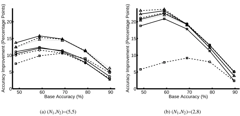
Simulating Multi-Cell Images We are interested in the simultaneous classification of all of the cells in a multi-cell microscope image. Unfortunately, it is difficult to collect multi-cell images for which we know the ground truth classification of each cell: if we prepare a slide from a mixture of two or more types of cells, we do not have direct control over which type appears where. For this reason, we simulated the multi-cell problem by creating synthetic multi-cell images using multiple real single-cell HeLa images.1 To generate a structured classification problem, we selected two of the ten classes at random; then we selected N1images from the first class and N2 from the second, with N1+N2=12. We then treated these images as if they were the output of a segmentation algorithm that was run on a multi-cell image.
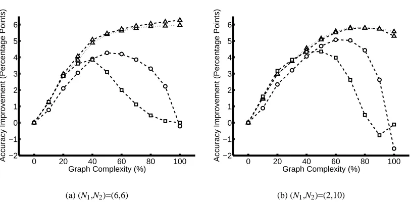
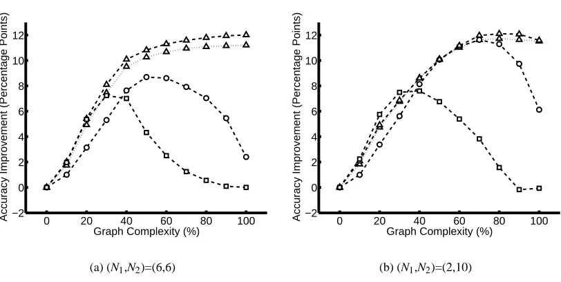
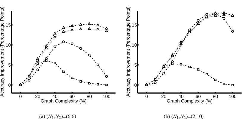
Constructing the Similarity Graph As an intermediate step in the construction of our factor graph, we built a similarity graph: the nodes of this graph correspond to cells, and an edge between two cells means that we believe that they are likely to share the same label. The simplest approach to building the similarity graph is to include all possible edges. With a fully-connected similarity graph, all cells in the test image are considered equally similar to one another; such a graph expresses a prior belief that images containing a few groups of same-class cells are more likely than images containing cells of many different classes. Our experiments below show that even this modest amount of prior information can improve the accuracy of our classifier compared to the no-edges (independent classification) case; for example, in Figs. 7–9, the performance of LBVP is higher
−5 0 5 −3
−2 −1 0 1 2 3
x axis
y axis
(a) Training Stage
−5 0 5
−3 −2 −1 0 1 2 3
x axis
y axis
(b) Testing Stage
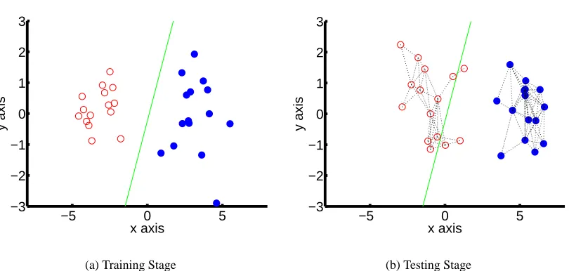
Figure 5: Classification of multiple examples using proximity in feature space. (a) At the training stage, a linear classifier separates two classes in a 2D feature space. (b) At the testing stage, we have added feature bias, causing 3 examples of one class to be misclassified. But, these examples can be classified correctly by constructing a similarity graph and running belief propagation on the corresponding factor graph.
when 100% of edges are present than it is when 0% of edges are present. But of course, if more-specific information is available, we will get better performance by using it to construct a more informative similarity graph with an intermediate number of edges.
One possible source of additional information is physical proximity between cells. Physical proximity is informative if we believe that nearby cells are likely to share an ancestor. However, we wanted to avoid having to simulate cell positions in our synthetic images, so in the current work we did not include edges based on physical proximity. In previous work (Chen and Murphy, 2006), we did evaluate graphs built using physical proximity, and they improved classification accuracy when applicable. So long as edges tend to connect cells that share the same class, the exact source of edges does not matter for our inference algorithms; so, the experimental results below should apply equally well to graphs that contain edges from physical proximity.
Instead, for our experiments below, we built the similarity graph according to feature-space proximity: we added edges between cells whose feature vectors were close to one another according to z-scored Euclidean distance. Using feature-space proximity in this way makes sense because minor experimental variations can perturb the features of a whole group of test cells in similar ways.
of the same class. So, as long as the feature bias is not so large that it causes most cells of a given class to be misclassified, we can hope to “rescue” cells that have been moved just across the class boundary, since they will be connected to other cells of the same class that are correctly classified. Fig. 5 justifies this intuition with a simple synthetic example.
In addition to the above reasons, feature-space proximity among test images could be infor-mative if the training set wasn’t large enough or the classifier wasn’t flexible enough to learn the location classes well. In our experiments, we believe that the influence of this last effect is minimal. To produce a variety of graphs with different edge densities, we introduced a parameter dcutoff: we connected two nodes whenever their z-scored Euclidean distance in feature space was less than dcutoff.2 Large values of dcutoffcorrespond to graphs with many edges, while small values correspond to graphs with few edges. We varied dcutoff to produce graphs with edge densities ranging from 0% to 100% of the possible edges.
Constructing the Factor Graphs From each similarity graph we built several different factor graphs using different kinds of potentials. Each different factor graph corresponds to a different way to turn our qualitative similarity judgements into a precise probability distribution over label vectors.
The simplest factor graph was the Potts model. In the Potts model, we used one Potts potential for each edge in the similarity graph; each potential had parameterω=1.7. The next type of factor graph was an associative Markov network. In this model we used one AMN potential for each node; this potential covered the node and all of its similarity-graph neighbors, and hadωy=2.9 for all y. The last type of factor graph used the voting potential. In this graph there was one voting potential centered on each node; this potential covered the node and all of its similarity-graph neighbors, and had parameterλ=1.7. For all three types of potential, we determined the above parameter values ahead of time by a coarse search.3
Synthetic Graphs Since the size of the 2D HeLa data set is limited, we performed additional experiments on automatically-generated inference problems. These experiments investigated the sensitivity of our method to the accuracy of the base classifier. We generated a synthetic graph by picking two of the ten classes at random and two numbers N1and N2. We generated N1cells of the first class and N2cells of the second. For each cell we selected feature vectors of length d=2 from a standard normal distribution; for one of the groups of cells we then displaced the feature vectors by a distance s. We chose s=3 as a value which yielded a reasonable degree of overlap between classes. Finally, as above, we connected pairs of nodes whose feature-space distances were less than dcutoff.
Synthetic Evidence To generate the evidence for a node in one of our synthetic graphs, we picked random scores for each class. The score for the true class was generated from a normal distribution
2. A reviewer of a previous version of this paper suggested that all edges should be present in the graph, and that we should adjust the weight of each edge based on the distance between the nodes. This is a reasonable suggestion; however, some of the potential functions we are evaluating do not have an obvious way to take edge weights into account. So, for the sake of an easier comparison, in this paper we work only with 0-1 weights.
3. As we examined the parameter space of the AMN potential, we discovered that results appear to be very sensitive to
the strength parameterωand the edge density of the graph. So, while we fixed a single compromise parameter for the