Learning Bounded Treewidth Bayesian Networks

Learning Bounded Treewidth Bayesian Networks

Gal Elidan [email protected]

Department of Statistics Hebrew University Jerusalem, 91905, Israel

Stephen Gould [email protected]

Department of Electrical Engineering Stanford University

Stanford, CA 94305, USA

Editor: David Maxwell Chickering

Abstract

With the increased availability of data for complex domains, it is desirable to learn Bayesian net-work structures that are sufficiently expressive for generalization while at the same time allow for tractable inference. While the method of thin junction trees can, in principle, be used for this pur-pose, its fully greedy nature makes it prone to overfitting, particularly when data is scarce. In this work we present a novel method for learning Bayesian networks of bounded treewidth that employs global structure modifications and that is polynomial both in the size of the graph and the treewidth bound. At the heart of our method is a dynamic triangulation that we update in a way that facilitates the addition of chain structures that increase the bound on the model’s treewidth by at most one. We demonstrate the effectiveness of our “treewidth-friendly” method on several real-life data sets and show that it is superior to the greedy approach as soon as the bound on the treewidth is nontrivial. Importantly, we also show that by making use of global operators, we are able to achieve better generalization even when learning Bayesian networks of unbounded treewidth.

Keywords: Bayesian networks, structure learning, model selection, bounded treewidth

1. Introduction

Recent years have seen a surge of readily available data for complex and varied domains. Accord-ingly, increased attention has been directed towards the automatic learning of large scale proba-bilistic graphical models (Pearl, 1988), and in particular to the learning of the graph structure of a Bayesian network. With the goal of making predictions or providing probabilistic explanations, it is desirable to learn models that generalize well and at the same time have low inference complexity or a small treewidth (Robertson and Seymour, 1987).

exponential in the treewidth bound (e.g., Karger and Srebro, 2001; Chechetka and Guestrin, 2008). In the context of general Bayesian networks, Bach and Jordan (2002) propose a local greedy ap-proach that upper bounds the treewidth of the model at each step. Because evaluating the bound on the treewidth of a graph is super-exponential in the treewidth (Bodlaender, 1996), their approach relies on heuristic techniques for producing tree-decompositions (clique trees) of the model at hand, and uses that decomposition as an upper bound on the true treewidth of the model. This approach, like standard structure search, does not provide guarantees on the performance of the model, but is appealing in its ability to efficiently learn Bayesian networks with an arbitrary treewidth bound.

While tree-decomposition heuristics such as the one employed by Bach and Jordan (2002) are efficient and useful on average, there are two concerns when using such a heuristic in a fully greedy manner. First, even the best of heuristics exhibits some variance in the treewidth estimate (see, for example, Koster et al., 2001) and thus a single edge modification can result in a jump in the treewidth estimate despite the fact that adding a single edge to the network can increase the true treewidth by at most one. More importantly, most structure learning scores (e.g., BIC, MDL, BDe, BGe) tend to learn spurious edges that result in overfitting when the number of samples is relatively small, a phenomenon that is made worse by a fully greedy approach. Intuitively, to generalize well, we want to learn bounded treewidth Bayesian networks where structure modifications are globally beneficial (contribute to the score in many regions of the network).

In this work we propose a novel approach for efficiently learning Bayesian networks of bounded treewidth that addresses these concerns. At the heart of our method is the idea of dynamically updat-ing a valid moralized triangulation of our model in a particular way, and usupdat-ing that triangulation to upper bound the model’s treewidth. Briefly, we use a novel triangulation procedure that is treewidth-friendly: the treewidth of the triangulated graph is guaranteed to increase by at most one when an edge is added to the Bayesian network. Building on the single edge triangulation, we are also able to characterize sets of edges that jointly increase the treewidth of the triangulation by at most one. We make use of this characterization of treewidth-friendly edge sets in a dynamic programming ap-proach that learns the optimal treewidth-friendly chain with respect to a node ordering. Finally, we learn a bounded treewidth Bayesian network by iteratively augmenting the model with such chains. Importantly, instead of local edge modifications, our method progresses by making use of chain structure operators that are more globally beneficial, leading to greater robustness and improving our ability to generalize. At the same time, we are able to guarantee that the bound on the model’s treewidth grows by at most one at each iteration. Thus, our method resembles the global nature of the method of Chow and Liu (1968) more closely than the thin junction tree approach of Bach and Jordan (2002), while being applicable in practice to any desired treewidth.

We evaluate our method on several challenging real-life data sets and show that our method is able to learn richer models that generalize better on test data than a greedy variant for a range of treewidth bounds. Importantly, we show that even when models with unbounded treewidth are learned, by employing global structure modification operators, we are better able to cope with the problem of local maxima in the search and learn models that generalize better.

our triangulation procedure. We evaluate the merits of our method in Section 8 and conclude with a discussion in Section 9.

2. Background

In this section we provide a basic review of Bayesian Networks as well as introduce the graph theoretic concepts of treewidth-decompositions and treewidth.

2.1 Bayesian Networks

Consider a finite set

X

={X1, . . . ,Xn}of random variables. A Bayesian network (Pearl, 1988) is an annotated directed acyclic graph that encodes a joint probability distribution over

X

. Formally, a Bayesian network over

X

is a pair B=h

G

,Θi. The first component,

G

= (V,E), is a directed acyclic graph whose vertices V correspond to the random variables in

X

. The edges E in the graph represent direct dependencies between the variables. The graph

G

represents independence properties that are assumed to hold in the underlying distribution: each Xi is independent of its non-descendants given its parents Pai ⊂

X

denoted by(Xi⊥NonDescendantsi|Pai). The second component,Θ, represents the set of parameters that quantify the network. Each node is annotated with a conditional probability distribution P(Xi |Pai), representing the conditional probability of the node Xigiven its parents in

G

, defined by the parametersΘXi|Pai. A Bayesian network defines a unique joint probability distribution over

X

given by

P(X1, . . . ,Xn) = n

∏

i=1

P(Xi|Pai).

A topological ordering

O

T of variables with respect to a Bayesian network structure is an ordering where each variable appears before all of its descendants in the network.

Given a Bayesian network model, we are interested in the task of probabilistic inference, or evaluating queries of the form PB(Y |Z) where Y and Z are arbitrary subsets of

X

. This task is, in general, NP-hard (Cooper, 1990), except when

G

is tree structured. The actual complexity of inference in a Bayesian network (whether by variable elimination, by belief propagation in a clique tree, or by cut-set conditioning on the graph) is proportional to its treewidth (Robertson and Seymour, 1987) which, roughly speaking, measures how closely the network resembles a tree (see Section 2.2 for more details).

Given a network structure

G

, the problem of learning a Bayesian network can be stated as follows: given a training set

D

={x[1], . . . ,x[M]}of instances of X⊆

X

, we want to learn parameters for the network. In the Maximum Likelihood setting we want to find the parameter values θthat maximize the log-likelihood function

log P(

D

|

G

,θ) =

∑

m

log P(x[m]|

G

,θ).

Learning the structure of a network poses additional challenges as the number of possible struc-tures is super-exponential in the number of variables and the task is, in general, NP-hard (Chicker-ing, 1996; Dasgupta, 1999; Meek, 2001). In practice, structure learning is typically done using a local search procedure, which examines local structure changes that are easily evaluated (add, delete or reverse an edge). This search is usually guided by a scoring function such as the MDL principle based score (Lam and Bacchus, 1994) or the Bayesian score (BDe) (Heckerman et al., 1995). Both scores penalize the likelihood of the data to limit the model complexity. An important characteristic of these scoring functions is that when the data instances are complete the score is decomposable. More precisely, a decomposable score can be rewritten as the sum

Score(

G

:

D

) =

∑

i

FamScoreXi(Pai :

D

).

where FamScoreXi(Pai :

D

) is the local contribution of Xi to the total network score. This term depends only on values of Xiand PaXi in the training instances.

Chow and Liu (1968) showed that maximum likelihood trees can be learned efficiently via a maximum spanning tree whose edge weights correspond to the empirical information between the two variables corresponding to the edge’s endpoints. Their result can be easily generalized for any decomposable score.

2.2 Tree-Decompositions and Treewidth

The notions of tree-decompositions (or clique trees) and treewidth were introduced by Robertson and Seymour (1987).1

Definition 2.1: A tree-decomposition of an undirected graph

H

= (V,E)is a pair({Ci}i∈T,

T

)with

{Ci}i∈T a family of subsets of V , one for each node of

T

, and

T

a tree such that

• S

i∈TCi=V .

• for all edges(v,w)∈E there exists an i∈

T

with v∈Ci and w∈Ci.

• for all i,j,k∈

T

: if j is on the (unique) path from i to k in

T

, then Ci∩Ck⊆Cj.

The treewidth of a tree-decomposition ({Ci}i∈T,

T

) is defined to be maxi∈T |Ci| −1. The treewidth TW(

H

) of an undirected graph

H

is the minimum treewidth over all possible tree-decompositions of

H

. An equivalent notion of treewidth can be phrased in terms of a graph that is a triangulation of

H

.

Definition 2.2: An induced path

P

=p1—p2. . .pLin an undirected graph

H

is a path such that for every non-adjacent pi,pj∈

P

there is no edge(pi—pj)in

H

. An induced (non-chordal) cycle is an induced path whose endpoints are the same vertex.

Definition 2.3: A triangulated or chordal graph is an undirected graph that has no induced cycles. Equivalently, it is an undirected graph in which every cycle of length greater than three contains a chord.

1. The properties defining a tree-decomposition are equivalent to the corresponding family preserving and running

It can be easily shown (Robertson and Seymour, 1987) that the treewidth of a given triangulated graph is the size of the maximal clique of the graph minus one. The treewidth of an undirected graph

H

is then equivalently the minimum treewidth over all possible triangulations of

H

.

For the underlying directed acyclic graph of a Bayesian network, the treewidth can be charac-terized via a triangulation of the moralized graph.

Definition 2.4: A moralized graph

M

of a directed acyclic graph

G

is an undirected graph that includes an edge(i— j)for every edge (i→ j) in

G

and an edge(p—q) for every pair of edges (p→i),(q→i)in

G

.

The treewidth of a Bayesian network graph

G

is defined as the treewidth of its moralized graph

M

, and corresponds to the complexity of inference in the model. It follows that the maximal clique of any moralized triangulation of

G

is an upper bound on the treewidth of the model, and thus its inference complexity.2

3. Learning Bounded Treewidth Bayesian Networks: Overview

Our goal is to develop an efficient algorithm for learning Bayesian networks with an arbitrary treewidth bound. As learning the optimal such network is NP-hard (Dagum and Luby, 1993), it is important to note the properties that we would like our algorithm to have. First, we would like our algorithm to be provably polynomial in the number of variables and in the desired treewidth. Thus, we cannot rely on methods such as that of Bodlaender (1996) to verify the boundedness of our network as they are super-exponential in the treewidth and are practical only for small treewidths. Second, we want to learn networks that are non-trivial. That is, we want to ensure that we do not quickly get stuck in local maxima due to the heuristic employed for bounding the treewidth of our model. Third, similar to the method of Chow and Liu (1968), we want to employ global structure operators that are optimal in some sense. In this section we present a brief high-level overview of our algorithm. In the next sections we provide detailed description of the different components along with proof of correctness and running time guarantees.

At the heart of our method is the idea of using a dynamically maintained moralized triangulated graph to upper bound the treewidth of the current Bayesian network. When an edge is added to the Bayesian network we update this (moralized) triangulated graph in a particular manner that is not only guaranteed to produce a valid triangulation, but that is also treewidth-friendly. That is, our update is guaranteed to increase the size of the maximal clique of the triangulated graph, and hence the treewidth bound, by at most one. As we will see, the correctness of our treewidth-friendly edge update as well as the fact that we can carry it out efficiently will both directly rely on the dynamic nature of our method. We discuss our edge update procedure in detail in Section 4.

An important property of our edge update is that we can characterize the parts of the network that are “contaminated” by the update by using the notion of blocks (bi-connected components) in the triangulated graph. This allows us to define sets of edges that are jointly treewidth-friendly. That is, these edge sets are guaranteed to increase the treewidth of the triangulated graph by at most one when all edges in the set are added to the Bayesian network structure. We discuss multiple edge updates in Section 5.

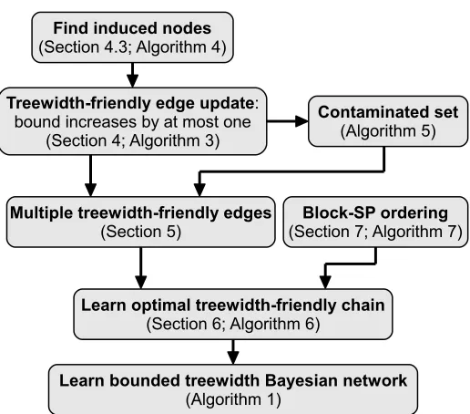
Figure 1: The building blocks of our method for learning Bayesian networks of bounded treewidth and how they depend on each other.

Building on the characterization of treewidth-friendly sets, we propose a dynamic programming approach for efficiently learning the optimal treewidth-friendly chain with respect to a node order-ing. We present this procedure in Section 6. To encourage chains that are rich in structure (have many edges), in Section 7 we propose a block shortest-path node ordering that is motivated by the properties of our triangulation procedure.

Finally, we learn Bayesian networks with bounded treewidth by starting with a Chow-Liu tree (Chow and Liu, 1968) and iteratively applying a global structure modification operator where the current structure is augmented with a treewidth-friendly chain that is optimal with respect to the ordering chosen. Appealingly, as each global modification can increase our estimate of the treewidth by at most one, if our bound on the treewidth is K, at least K such chains will be added before we even face the problem of local maxima. In practice, as some chains do not increase the treewidth, many more such chains are added for a given maximum treewidth bound. Figure 1 illustrates the relationship between the different components of our approach.

Algorithm (1) shows pseudo-code of our method. Briefly, Line 4 initializes our model with a Chow and Liu (1968) tree; Line 8 produces a node ordering given the model at hand; Line 9 finds the optimal chain with respect to that ordering; and Line 10 augments the current model with the new edges. We then use our treewidth-friendly edge update procedure to perform the moralization and triangulation on

M

+for each edge added to the Bayesian network

G

(Line 12). Once the maximal clique size reaches the treewidth bound K, we continue to add edges greedily until no more edges can be added without increasing the treewidth (Line 16).

Algorithm 1: Learning A Bayesian Network with Bounded Treewidth

Input :

D

// training set

1

K // maximum treewidth

2

Output:

G

// a graph structure with treewidth at most K

3

G

←maximum scoring spanning tree

4

M

+_{←undirected skeleton of}

_G

5

k←1

6

while k<K and positive scoring edges exist do

7

O

←node ordering given

G

and

M

+ // Algorithm (7)

8

C

←maximum scoring chain with respect to

O

// Algorithm (6)

9

G

←

G

∪

C

10

foreach(i→ j)∈

C

do

11

M

+_{←EdgeUpdate(}

_M

+_{,(i→ j)) // Algorithm (3)}

12

end foreach

13

k←maximal clique size of

M

+

14

end

15

Greedily add edges to

G

that do not increase treewidth beyond K

16

return

G

17

We will prove this result gradually using the developments of the next sections. Note that we will show that our method is guaranteed to be polynomial both in the size of the graph and the treewidth bound. Thus, like the greedy thin junction tree approach of Bach and Jordan (2002), it can be used to learn a Bayesian networks given an arbitrary treewidth bound. It is also important to note that, as in the case of the thin junction tree method, the above result is only useful if the actual Bayesian network learned is expressive enough to be useful for generalization. As we will demonstrate in Section 8, by making use of global treewidth-friendly updates, our method indeed improves on the greedy approach and learns models that are rich and useful in practice.

4. Treewidth-Friendly Edge Update

In this section we consider the basic building block of our method: the manner in which we update the triangulated graph when a single edge is added to the Bayesian network structure. Throughout this section we will build on the dynamic nature of our method and make use of the valid moralized triangulation graph that was constructed before adding an edge (s→t) to the Bayesian network structure. We will start by augmenting it with(s—t)and any edges required for moralization. We will then triangulate the graph in a treewidth-friendly way, increasing the size of the maximal clique in the triangulated graph by at most one. For clarity of exposition, we start with a simple variant of our triangulation procedure in Section 4.1 and refine it in Section 4.2.

4.1 Single-source Triangulation

Algorithm 2: SingleSourceEdgeUpdate: Update of

M

+when adding(s→t)to

G

Input :

M

+ // triangulated moralized graph of

G

1

(s→t) // edge to be added to

G

2

Output:

M

+_(s→t) // a triangulated moralized graph of

G

∪(s→t)

3

M

+

(s→t)←

M

+∪(s—t)

4

foreach p∈Pat do 5

M

+

(s→t)←

M

+(s→t)∪(s—p)// moralization

6

end foreach

7

foreach node v on an induced path between s and t∪Pat in

M

+do 8

M

+

(s→t)←

M

+(s→t)∪(s—v)

9

end foreach

10

return

M

+₍s→t)

11

s

t p

t p s

t p s

t p s

(a) Bayesian network (b) Addition of (c) Addition of (d) Addition of the

G

∪(s→t) (s—t)to

M

+ moralizing edges triangulating edges

(line 4) (lines 5-7) (lines 8-10)

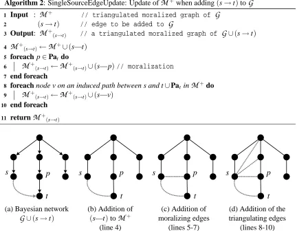
Figure 2: Example showing the application of the single-source triangulation procedure of Algo-rithm (2) to a simple graph. The treewidth of the original graph is one, while the graph augmented with(s→t)has a treewidth of two (maximal clique of size three).

Observation 4.1: Let

G

be a Bayesian network structure and let

M

+ be a moralized triangulation of

G

. Let

M

(s→t) be

M

+ augmented with the edge (s—t) and with the edges (s—p) for every

parent p of t in

G

. Then, every non-chordal cycle in

M

_(s→t)involves s and either t or a parent of t and an induced path between the two vertices.

Stated simply, if the graph was triangulated before the addition of (s→t) to the Bayesian network, then we only need to triangulate cycles created by the addition of the new edge or those forced by moralization. This observation immediately suggests the straight-forward single-source triangulation outlined in Algorithm (2): add an edge (s—v) for every node v on an induced path between s and t or s and a parent p of t before the edge update. Figure 2 shows an application of the procedure to a simple graph. Clearly, this naive method results in a valid moralized triangulation of

G

∪(s→t). Surprisingly, we can also show that it is treewidth-friendly.

Proof: Let C be the nodes in any maximal clique

M

+. We consider the minimal set of edges required to increase the size of C by more than one and show that this set cannot be a subset of the edges added by our single-source triangulation. In order for the clique to grow by more than one node, at least two nodes i and j not originally in C must become connected to all nodes in C. Since there exists at least one node k∈C that is not adjacent to i and similarly there exists at least one node l∈C not adjacent to j, both edges(i—k)and(j—l)are needed to form the larger clique. There are two possibilities illustrated below (the dotted edges are needed to increase the treewidth by two and all other edges between i,j and the current maximal clique are assumed to exist):

C

i j

k, l

C

i j

k l

(a)(i— j)does not exist (b)(i— j)exists

• (i— j)does not exist (a). In this case k and l can be the same node but the missing edge (i— j)is also required to form the larger clique.

• (i— j)exists (b). In this case k and l cannot be the same node or the original clique was not maximal since C∪i∪j\k would have formed a larger clique. Furthermore one of k or l must not be connected to both i and j otherwise i— j—k—l—i forms a non-chordal cycle of length four contradicting our assumption that the original graph was triangulated. Thus, in this case either(i—l)or(j—k)are also required to form the larger clique.

In both scenarios, at least two nodes have two incident edges and the three edges needed cannot all be incident to a single vertex. Now consider the triangulation procedure. Since, by construction, all edges added in Algorithm (2) emanate from s, the above condition (requiring two nodes to have two incident edges and the three edges not all incident to a single vertex) is not met and the size of the maximal clique in the new graph cannot be larger than the size of the maximal clique in

M

+by more than one. It follows that the treewidth of the moralized triangulated graph cannot increase by more than one.

(a) Chain network (b) Triangulation after (c) Triangulation after (d) Alternative (v1→v6)is added (v2→v5)is added triangulation

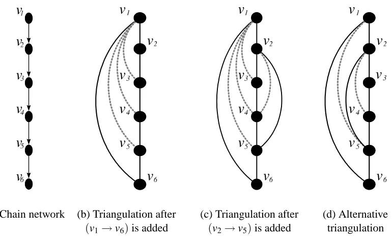
Figure 3: Example demonstrating that the single-source edge update of Algorithm (2) can be prob-lematic for later edge additions. (a) shows a simple six nodes chain Bayesian network; (b) a single-source triangulation when(v1→v6)is added to the network with a treewidth of two; (c) a single-source triangulation when in addition(v2→v5)is added to the model with a treewidth of three; (d) an alternative triangulation to (b). This triangulation already includes the edge (v2—v5) and the moralizing edge (v2—v4) and thus is also a valid moralized triangulation after(v2→v5)has been added, but has a treewidth of only two.

4.2 Alternating Cut-vertex Triangulation

To refine the single-source triangulation discussed above with the goal of addressing the problem exemplified in Figure 3 we make use of the concepts of cut-vertices, blocks, and block trees (see, for example, Diestel, 2005).

Definition 4.3: A block, or biconnected component, of an undirected graph is a set of connected nodes that cannot be disconnected by the removal of a single vertex. By convention, if the edge (u—v)is in the graph then u and v are in the same block. Vertices that separate (are in the intersec-tion of) blocks are called cut-vertices.

It follows directly from the definition that between every two nodes in a block (of size greater than two), there are at least two distinct paths, that is, a cycle. There are also no simple cycles involving nodes in different blocks.

Definition 4.4: A block tree

B

of an undirected graph

H

is a graph with nodes that correspond both to cut-vertices and to blocks of

H

. The edges in the block tree connect any block node Bi with a cut-vertex node vjif and only if vj∈Biin

H

.

(a) Bayesian network,

G

(b) A possible triangulated graph,

M

+

(c) Unique block tree,

B

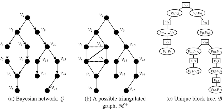
Figure 4: Example of a Bayesian network with a corresponding moralized triangulated graph and the unique block tree. Boxes in the block tree denote cut-vertices, ellipses denote blocks.

in different blocks passes through all the cut-vertices along the path between the blocks in

B

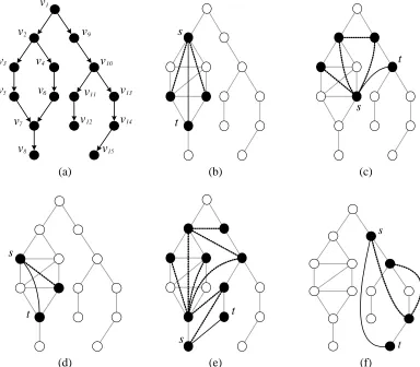
. An important consequence that directly follows from the result of Dirac (1961) is that an undirected graph whose blocks are triangulated is overall triangulated.

We can now describe our improved treewidth-friendly triangulation outlined in Algorithm (3) and illustrated via an example in Figure 5. First, the triangulated graph is augmented by the edge (s—t) and any edges needed for moralization (Figure 5(b) and (c)). Second, if s and t are not in the same block, a block level triangulation is carried out by starting from s and zig-zagging across the cut-vertices along the unique path between the blocks containing s and t and its parents in the block tree (Figure 5(d)). Next, within each block along the path (not containing s or t), a chord is added between the “entry” and “exit” cut-vertices along the block path, thereby short-circuiting any other node path through the block. In addition, within each such block we perform a single-source triangulation with respect to s0by adding an edge(s0—v)between the first cut-vertex s0and any node v on an induced path between s0 and the second cut-vertex t0. The block containing s is treated the same as other blocks on the path with the exception that the short-circuiting edge is added between s and the first cut-vertex along the path from s to t. For the block containing t and its parents, instead of adding a chord between the entry cut-vertex and t, we add chords directly from s to any node v (within the block) that is on an induced path between s and t (or parents of t) (Figure 5(e)). This is required to prevent moralization and triangulation edges from interacting in a way that will increase the treewidth by more than one (see Figure 5(f) for an example). If s and t happen to be in the same block, then we only triangulate the induced paths between s and t, that is, the last step outlined above. Finally, in the special case that s and t are in disconnected components of

G

, the only edges added are those required for moralization.

Algorithm 3: EdgeUpdate: Update of

M

+when adding(s→t)to

G

Input :

M

+ // triangulated moralized graph of

G

1

O

// node ordering

2

(s→t) // edge to be added to

G

3

Output:

M

+(s→t) // a triangulated moralized graph of

G

∪(s→t)

4

B

←block tree of

M

+

5

M

+

(s→t)←

M

+∪(s—t)

6

foreach p∈Pat do 7

M

+

(s→t)←

M

+(s→t)∪(s—p)// moralization

8

end foreach

9

// triangulate (cut-vertices) between blocks

C

={c1, . . . ,cM} ←sequence of cut-vertices on the path from s to t∪Pat in block tree

B

10

Add(s—cM),(cM—c1),(c1—cM−1),(cM−1—c2), . . .to

M

+(s→t)

11

// triangulate nodes within blocks on path from s to t∪Pat

E

← {(s—c1),(c1—c2), . . . ,(cM−1—cM)} 12

foreach edge(s0—t0)∈

E

do

13

M

+

(s→t)←

M

+(s→t)∪(s0—t0)

14

foreach node v on an induced path between s0and t0in the original block containing

15

both do

M

+

(s→t)←

M

+(s→t)∪(s0—v)

16

end foreach

17

end foreach

18

// triangulate s with nodes in block containing t∪Pat

foreach node v on an induced path between s and t∪Pat in the new block containing them 19

do

M

+

(s→t)←

M

+(s→t)∪(s—v)

20

end foreach

21

return

M

+(s→t)

22

Observation 4.5: (Family Block). Let u be a node in a Bayesian network

G

and let Paube the set of parents of u. Then the block tree for any moralized triangulated graph

M

+ of

G

has a unique block containing{u,Pau}.

Observation 4.6: (Path Nodes). Let

B

= ({Bi} ∪ {cj},

T

)be the block tree of

M

+with blocks

{Bi}and cut-vertices{cj}. Let s and t be nodes in blocks Bsand Bt, respectively. If t is a cut-vertex then let Bt be the (unique) block that also contains Pat. If s is a cut-vertex, then choose Bsto be the block containing s closest to Bt in

T

. Then a node v is on a path from s to t or from s to a parent of

t if and only if it is in a block that is on the unique path from Bsto Bt.

(a) Bayesian network,

G

augmented with(s→t)

(b) Moralized graph augmented with(s—t)

(c) Addition of moralizing edges to Pat

(d) Addition of between-block zigzag edges

(e) Addition of within-block triangulation edges (Complete

triangulation from s)

(f) An alternative final triangulation from cM

Figure 5: Example showing our triangulation procedure (b)-(e) for s and t in different blocks. (The blocks are{s,v1},{v1,cM}, and{cM,v2,v3,p1,p2,t}with corresponding cut-vertices v1 and cM). The original graph has a treewidth of two, while the graph augmented with (s→t)has treewidth three (maximal clique of size four). An alternative triangulation (f), connecting cMto t, however, would result in a clique of size five{s,cM,p1,p2,t}.

is,{v2,v1,v9}. We can now use these properties to show that our edge update procedure produces a valid triangulation.

Lemma 4.7: If

M

+is a valid moralized triangulation of the graph

G

then Algorithm (3) produces a moralized triangulation

M

+(s→t)of the graph

G

(s→t)≡

G

∪(s→t).

Proof: Since

M

+was triangulated, every cycle of length greater than or equal to four in

G

(s→t)is

the result of the edge (s—t) or one of the moralizing edges, together with an induced path (path with no shortcuts) between the endpoints of the edge. We consider three cases:

• s and t are disconnected in

M

+: There are no induced paths between s and t so the only edges required are those for moralization. These edges do not produce any induced cycles.

t and s. Otherwise, t is a cut-vertex between the block that contains its parents and the block that contains s. It follows that all paths (including induced ones) from a parent of t to s pass through t and the edges added for the s,t-block triangulate all newly created induced cycles that result from the moralizing edges.

• s and t are not in the same block: As noted in Observation 4.6, all paths in

M

+ from s to t or a parent of t pass through the unique cut-vertex path from the block containing s to the block containing t and its parents. The edges added in Line 14 short-circuit the in-going s0 and out-going t0 of each block creating a path containing only cut-vertices between s and t. Line 11 triangulates this path by forming cycles of length three containing s0, t0and some other cut-vertex. The only induced cycles remaining are contained within blocks and contain the newly added edge(s0—t0)or involve the edge between s and the last cut-vertex(s—cM) and one of the edges between s and t or a parent of t. It follows that within-block triangulation with respect to s0 and t0 will shortcut the former induced cycles, and the edges added from s in Line 20 will shortcut the later induced cycles.

To complete the proof, we need to show that any edge added from s (or s0) to an induced node v does not create new induced cycles. Any such induced cycle would have to include an induced path from the endpoints of the edge added and thus would have been a sub-path of some induced cycle that includes both s and v. This cycle would have already been triangulated by our procedure.

Having shown that our update produces a valid triangulation, we now prove that our edge update is indeed treewidth-friendly and that it can increase the treewidth of the moralized triangulated graph by at most one.

Theorem 4.8: The treewidth of the output graph

M

+(s→t) of Algorithm (3) is greater than the

treewidth of the input graph

M

+by at most one.

Proof: As shown in the proof of Theorem 4.2, the single-source triangulation within a block is guar-anteed not to increase the maximal clique size by more than one. In addition, from the properties of blocks it follows directly that the inner block triangulation does not add edges that are incident to nodes outside of the block. It follows that all the inner block single-source triangulations indepen-dently effect disjoint cliques. Thus, the only way that the treewidth of the graph can further increase is via the zig-zag edges. Now consider two cliques in different blocks. Since our block level zig-zag triangulation only touches two cut-vertices in each block, it cannot join two cliques of size greater than two into a single larger one. In the simple case of two blocks with two nodes (a single edge) and that intersect at a single cut-vertex, a zig-zag edge can indeed increase the treewidth by one. In this case, however, there is no within-block triangulation and so the overall treewidth cannot increase by more than one.

4.3 Finding Induced Nodes

We finish the description of our edge update (Algorithm (3)) by showing that it can be carried out efficiently. That is, we have to be able to efficiently find the vertices on all induced paths between two nodes in a graph. In general, this task is computationally difficult as there are potentially exponentially many such paths between any two nodes. To cope with this problem, we again make use of the dynamic nature of our method.

Algorithm 4: InducedNodes: compute set of nodes on induced path between s0and t0in

M

+

Input :

M

+ // moralized triangulated graph

1

s0,t0 // two nodes in

M

+

2

Output:

I

// set of nodes on induced paths between s0 and t0

3

H

← block (subgraph) of

M

+∪(s0—t0)containing s0and t0

4

I

← /0 5

while edges being added do

6

// maximum cardinality search

X

← all nodes in

H

except s0

7

Y

← {s0} 8

while

X

6= /0do

9

Find v∈

X

with maximum number of neighbors in

Y

10

X

←

X

\ {v}and

Y

←

Y

∪ {v} // remove from

X

, add to

Y

11

if there exists u,w∈

Y

such that(u—w)∈/

H

then

12

I

←

I

∪ {u,v,w} 13

Add edges(s0—u),(s0—v)and(s0—w)to

H

14

Restart maximum cardinality search

15

end

16

end

17

end

18

return

I

19

after adding(s0—t0)to the graph, every cycle detected will involve an induced path between the two nodes. Using this observation, we can make use of the ability of the maximum cardinality search algorithm (Tarjan and Yannakakis, 1984) to iteratively detect non-chordal cycles.

The method is outlined in Algorithm (4). At each iteration we attempt to complete a maximum cardinality search starting from s0(Line 7 to Line 17). If the search fails, we add the node at which it failed, v, together with its non-adjacent neighboring nodes{u,w}to the set of induced nodes and augment the graph with triangulating edges from s0to each of{u,v,w}. If the search completes then we have successfully triangulated the graph and hence found all induced nodes. Note that using the properties of blocks and cut-vertices, we only need to consider the subgraph that is the block created after the addition of(s0—t0)to the graph.

Lemma 4.9: (Induced Nodes). Let

M

+be a triangulated graph and let s0and t0be any two nodes in

M

+. Then Algorithm (4) efficiently returns all nodes on any induced path between s0 and t0 in

M

+_{, unless those nodes are connected directly to s}0_.

a path must have been part of another cycle where v was an induced node and hence would have been triangulated.

Thus Algorithm (4) returns exactly the set of nodes on induced paths from s0 to t0 that s0 needs to connect to in order to triangulate the graph

M

+∪(s—t). The efficiency of our edge update procedure of Algorithm (3) follows immediately as all other operations are simple.

5. Multiple Edge Updates

In this section we define the notion of a contaminated set, or the subset of nodes that are incident to edges added to

M

+in Algorithm (3), and characterize sets of edges that are jointly guaranteed not to increase the treewidth of the triangulated graph by more than one. We begin by formally defining the terms contaminate and contaminated set.

Definition 5.1: We say that a node v is contaminated by the addition of the edge (s→t) to

G

if it is incident to an edge added to the moralized triangulated graph

M

+by a call to Algorithm (3). The contaminated set for an edge(s→t)is the set of all nodes v that would be contaminated (with respect to

M

+) by adding(s→t)to

G

, including s, t, and the parents of t.

Figure 6 shows some examples of contaminated sets for different edge updates. Note that our definition of contaminated set only includes nodes that are incident to new edges added to

M

+and, for example, excludes nodes that were already connected to s before(s→t)is added, such as the two nodes adjacent to s in Figure 6(b).

Using the separation properties of cut-vertices, one might be tempted to claim that if the con-taminated sets of two edges overlap at most by a single cut-vertex then the two edges jointly increase the treewidth by at most one. This however, is not true in general as the following example shows.

Example 5.2: Consider the Bayesian network shown below in (a) and its triangulation (b) after (v1→v4)is added, increasing the treewidth from one to two. (c) is the same for the case when (v4→v5)is added to the network. Despite the fact that the contaminated sets (solid nodes) of two edge additions overlap only by the cut-vertex v4, (d) shows that jointly adding the two edges to the graph results in a triangulated graph with a treewidth of three.

(a) (b) (c) (d)

(a) (b) (c)

(d) (e) (f)

Figure 6: Some examples of contaminated sets (solid nodes) that are incident to edges added (dashed) by Algorithm (3) for different candidate edge additions(s→t)to the Bayesian network shown in (a). In (b), (c), (d), and (e) the treewidth is increased by one; In (f) the treewidth does not change.

Theorem 5.3: (Treewidth-friendly pair). Let

G

be a Bayesian network graph structure and

M

+ be its corresponding moralized triangulation. Let(s→t)and(u→v)be two distinct edges that are topologically consistent with

G

. Then the addition of the edges to

G

does not increase the treewidth of

M

+ by more than one if one of the following conditions holds:

• the contaminated sets of(s→t)and(u→v)are disjoint.

• the endpoints of each of the two edges are not in the same block and the block paths between the endpoints of the two edges do not overlap and the contaminated sets of the two edge overlap at a single cut-vertex.

Algorithm 5: ContaminatedSet: compute contaminated set for(s→t)

Input :

G

// Bayesian network

1

M

+ _{// moralized triangulated graph}

2

(s→t) // candidate edge

3

Output:

C

s,t // contaminated set for (s→t) 4

C

s,t← {s,t} ∪ {p∈Pat |(s—p)∈/

M

+} 5

foreach edge(s0—t0)∈

E

in procedure Algorithm (3) with(s0—t0)∈/

M

+_do

6

I

=InducedNodes(

M

+,{s0,t0})

7

C

s,t←

C

s,t∪ {v∈

I

|(s0—v)∈/

M

+} 8

end foreach

9

H

← {s}and block containing t∪Pat 10

H

←

H

∪ {(s—p)|p∈Pat} ∪(s—c)where c is the cut-vertex closest to s in the block 11

containing t

I

=InducedNodes(

H

,{s,t})

12

C

s,t←

C

s,t∪ {v∈

I

|(s0—v)∈/

M

+} 13

return

C

s,t 14

can only happen if the contamination sets of the two edge updates are not completely disjoint. Now, consider the case when the two sets overlap by a single cut-vertex. By construction all triangulating edges added are along the block path between the endpoints of each edge. Since the block paths of the two edge updates do not overlap there can not be an edge between a node in the contaminated set of (s→t) and the contaminated set of (u→v) (except for the single cut-vertex). But then no node from either contaminated set can become part of a clique involving nodes from the other contaminated set. Thus there are no two nodes that can be added to the same clique. It follows that the maximal clique size of

M

+, and hence the treewidth bound, cannot grow by more than one.

The following result is an immediate consequence.

Corollary 5.4: (Treewidth-friendly set). Let

G

be a Bayesian network graph structure and

M

+ be its corresponding moralized triangulation. If{(si→ti)}is a set of edges so that every pair of

edges satisfies the condition of Theorem 5.3 then adding all edges to

G

can increase the treewidth bound by at most one.

The above result characterizes treewidth-friendly sets. In the search for such sets that are useful for generalization (see Section 6), we will need be able to efficiently compute the contaminated set of candidate edges. At the block level, adding an edge between s and t in

G

can only contaminate blocks between the block containing s and that containing t and its parents in the block tree for

M

+ _{(Observation 4.6). Furthermore, identifying the nodes that are incident to moralizing edges}

6. Learning Optimal Treewidth-Friendly Chains

We now want to build on the results of the previous sections to facilitate the addition of global moves that are both optimal in some sense and are guaranteed to increase the treewidth by at most one. Specifically, we consider adding optimal chains that are consistent with some topological node ordering. On the surface, one might question the need for a specific node ordering altogether if chain global operators are to be used—given the result of Chow and Liu (1968), one might expect that learning the optimal chain with respect to any ordering can be carried out efficiently. However, Meek (2001) showed that learning such an optimal chain over a set of random variables is computationally difficult. Furthermore, conditioning on the current model, the problem of identifying the optimal chain is equivalent to learning the (unconditioned) optimal chain.3 Thus, during any iteration of our algorithm, we cannot expect to find the overall optimal chain.

Instead, we commit to a single node ordering that is topologically consistent and learn the optimal chain with respect to that order. In this section we will complete the development of our algorithm and show how we can efficiently learn chains that are optimal with respect to any such ordering. In Section 7 we will also suggest a useful node ordering motivated by the characteristics of contaminated sets. We start by formally defining the chains that we will learn.

Definition 6.1: A treewidth-friendly chain

C

with respect to a node ordering

O

is a chain with respect to

O

such that the contamination conditions of Theorem 5.3 hold for the set of edges in

C

.

Given a treewidth-friendly chain

C

to be added for Bayesian network

G

, we can apply the edge update of Algorithm (3) successively to every edge in

C

to produce a valid moralized triangulation of

G

∪

C

. The result of Theorem 5.4 ensures that the resulting moralized triangulation will have treewidth at most one greater than the original moralized triangulation

M

+.

To find the optimal treewidth-friendly chain in polynomial time, we use a straightforward dy-namic programming approach: the best treewidth-friendly chain that contains (

O

s→

O

t) is the concatenation of

• the best treewidth-friendly chain from the first node in the order

O

1to

O

F, the first ordered node contaminated by the edge(

O

s→

O

t)

• the edge(

O

s→

O

t)

• the best treewidth-friendly chain starting from

O

L, the last node contaminated by the edge (

O

s→

O

t), to the last node in the order,

O

N.

O₁ O_F O_s O_L O_N

optimal chain optimal chain

O_t

We note that when the end nodes are not separating cut-vertices, we maintain a gap so that the contamination sets are disjoint and the conditions of Theorem 5.3 are met.

Formally, we define C[i,j]as the optimal chain whose contamination starts at or after

O

i and ends at or before

O

j. To find the optimal treewidth-friendly chain with respect to a node ordering

O

for a Bayesian network with N variables, our goal is then to compute C[1,N]. Using the short-hand notation F to denote the first node ordered in the contamination set of(s→t)and L to denote the last ordered node in the contamination set, we can readily compute C[1,N]via the following recursive update principle

C[i,j] =max  



maxs,t:F=i,L=j(s→t) no split maxk=i+1: j−1C[i,k]∪C[k,j] split

/0 leave a gap

where the maximization is with respect to the score (e.g., BIC) of the structures considered. In simple words, the maximum chain in any sub-sequence[i,j]in the node ordering is the maximum of three alternatives: all edges whose contamination boundaries are exactly i and j (no split); all two chain combinations that are in the sub-sequence[i,j]and are joined at some node i<k< j (split); a gap between i and j in the case that there is no edge whose contamination is contained in this range and that increases the score.

Algorithm (6) outlines a simple backward recursion that computes C[1,N]. At each node, the algorithm maintains a list of the best partial chains evaluated so far that contaminates nodes up to, but not preceding, that node in the ordering. That is, the list of best partial chains is indexed by where the contamination boundary of each chain starts in the ordering. By recursing backwards from the last node, the algorithm is able to update this list by evaluating all candidate edges terminating at the current node. It follows that, once the algorithm iterates past a node t we have the optimal chain starting from that node. Thus, at the end of the recursion we are left with the optimal non-contaminating chain starting from the first node in the ordering.

The recursion starts at Line 7. If for node

O

t the best chain starting from the succeeding node

O

t+1 is better than the best chain starting from

O

t, we replace the best chain from

O

t with the one from

O

t+1 simply leaving a gap in the chain (Line 8). Then, for every edge terminating at

O

t, we find the first ordered node

O

F and the last ordered node

O

Lthat would be contaminated by adding that edge. If the score for the edge plus the score for the best partial non-contaminating chain from

O

F is better than the current best partial chain from

O

Lthen we replace the best chain from

O

Lwith the one just found (Line 19).

With the ability to learn optimal chains with respect to a node ordering, we have completed the description of all the components of our algorithm for learning bounded treewidth Bayesian network outlined in Algorithm (1). Its efficiency is a direct consequence of our ability to learn treewidth-friendly chains in time that is polynomial both in the number of variables and in the treewidth at each iteration. For completeness we now restate and prove Theorem 3.1.

Theorem 3.1: Given a treewidth bound K, Algorithm (1) runs in time polynomial in the number of variables and K.

Algorithm 6: LearnChain: learn optimal non-contaminating chain with respect to topological node ordering

Input :

O

// topological node ordering

1

Output:

C

// non-contaminating chain

2

// initialize dynamic programming data

for i=1 to|

O

|+1 do

3

bestChain[i]← /0 // best chain from i-th node

4

bestScore[i]←0 // best score from i-th node

5

end

6

// backward recursion

for t=|

O

|down to 1 do

7

if(bestScore[t+1]>bestScore[t])then

8

bestChain[t]←bestChain[t+1]

9

bestScore[t]←bestScore[t+1]

10

end

11

for s=1 to t−1 do // evaluate edges

12

V

←contaminated set for candidate edge(

O

s→

O

t) 13

f ←first ordered node in

V

// must be ≤s

14

l←last ordered node in

V

// must be ≥t

15

if bestChain[l].last and(

O

s→

O

t)do not satisfy the conditions of Theorem 5.3 then 16

l←l+1 // leave a gap

17

end

18

if(∆Score(

O

s→

O

t) +bestScore[l]>bestScore[f])then 19

bestChain[f]← {(

O

s→

O

t)} ∪bestChain[l] 20

bestScore[f]←∆Score(

O

s→

O

t) +bestScore[l] 21

end

22

end

23

end

24

// return optimal non-contaminating chain

return bestChain[1]

25

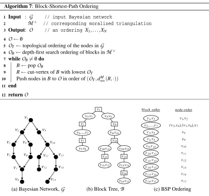
7. Block-Shortest-Path Ordering

In the previous sections we presented an algorithm for learning bounded treewidth Bayesian net-works given any topological ordering of the variables. In order to make the most of our method, we would like our ordering to facilitate rich structures that will have beneficial generalization proper-ties. Toward that end, in this section we consider the practical matter of a concrete node ordering. We will present a block shortest-path (BSP) node ordering that is motivated by the specific proper-ties of our triangulation method.4

To make our node ordering concrete, since the contamination resulting from edges added within an existing block is limited to the block, we start by grouping together all nodes that are within a block (cut-vertices that appear in multiple blocks are included in the first block chosen). Our node ordering is then a topologically consistent ordering over the blocks combined with a topologically consistent ordering over the nodes within each block. We use topological consistency to facilitate as many edges as possible though this is not required by the theory (and, in particular, Theorem 5.3).

We now consider how to order interchangeable blocks by taking into account that our triangu-lation following an edge addition(s→t)only involves variables that are in blocks along the unique path between the block containing s and the block containing t and its parents. The following example motivates a natural choice for this ordering.

Example 7.1: Consider a Bayesian network with root node R and three branches: R→A1→. . .→AL, R→B1→. . .→BN, and R→C1→. . .→CM. If we add an edge Ai →Bj to the network, then by the block contamination results, our triangu-lation procedure will touch (almost) every node on the path be-tween Ai and Bj. This implies that we can not include addi-tional edges of the type Bk →Cl in our chain since the block path from Bk to R overlaps with the block path from Bj to

R. Note, however, that any edge Cp→Cq>p is still allowed to be added since its contaminated set does not overlap with that of Ai → Bj. Now, consider the two obvious topologi-cal node orderings:

O

BFS= (R,A1,B1,C1,A2, . . .) and

O

DFS= (R,A1, . . . ,AL,B1, . . . ,BN,C1, . . .). Only the DFS ordering, ob-tained by grouping the Bi’s together, allows us to consider such edge combinations.

Motivated by the above example to order interchangeable blocks, we use a block level depth-first ordering. The question now is whether a further characterization of the contaminated set can be provided in order to better order topologically interchangeable nodes within a block. To answer this question we consider the following example.

Example 7.2: Consider the Bayesian network shown below whose underlying undirected structure is a valid moralized triangulation and forms a single block. Numbers in the boxes indicate the (undi-rected) distance of each node from r, a property that we make use of below.

r

v2

v1 v3 v4

v6

v5 v7 v8 v9

s

t

0 1

1

2 2

1 1

1

2 2 3

The single edge addition(s→t)will contaminate every node in the block (other than those already adjacent to it) since all nodes lie on induced paths between s and t. However other edge additions, such as(v3→t)have a much smaller contamination set:{v3,t}.

Based on the above example, one may think that no within-block ordering can improve the expected contamination of edges added, and that we may be forced to only add a single edge per block, making our method greedier than we would like. Fortunately, there is a straightforward way to characterize the within-block contamination set using the notion of shortest path length. Let

G

be a Bayesian network over variables

X

. We denote by dminM (u,v)the minimum distance (shortest

path) between nodes u,v∈

X

in

M

+. We note the following useful properties of dminM(·,·):

• dminM (u,v)≥0 with equality if and only if u=v

• dminM (u,w)+d

M

min(v,w)≥d

M

min(u,v)with equality if and only if w is on the (possibly non-unique)

shortest path between u and v

• if u and v are disconnected in

M

+then, by convention, dMmin(u,v) =∞

Theorem 7.3: Let r, s and t be nodes in some block B (of size≥3) in the triangulated graph

M

+ with dminM (r,s)≤d

M

min(r,t). Then for any v on an induced path between s and t we have dminM (r,v)≤d

M

min(r,t)

Proof: Since the nodes are all in the same block we know that there must be at least two paths between any two nodes. Let p and q be the shortest paths from nodes r to s and r to t, respectively (denoted r. . .p s and r. . .q t). If p and q meet at some node other than r then they will share the path from that node to r (otherwise they cannot be shortest paths). Let such a shared node furthest from r be r0. Then dMmin(r,t) =d

M

min(r,r

0_{) +d}M

min(r

0_{,t)and d}M

min(r,v)≤d

M

min(r,r

0_{) +d}M

min(r

0_{,v)so if the result}

holds for r0it holds for r. Without loss of generality assume that there is no such r0. Now consider the following cases:

• If q contains v then dMmin(r,v) =d

M

min(r,t)−d

M

min(v,t)<d

M

min(r,t).

• If p contains v then dminM(r,v) =d

M

min(r,s)−d

M

min(v,s)<d

M

min(r,s)≤d

M

min(r,t).

• Otherwise v is on some other (induced) path between s and t. But now r. . .p s. . .v. . .t. . .q r forms a cycle of length≥4. Since

M

+is triangulated there must be an edge from v to some node on p or q. There cannot be an edge between s and t or else there would not be any induced paths between s and t. But then dM

min(r,v)≤d

M

Algorithm 7: Block-Shortest-Path Ordering

Input :

G

// input Bayesian network

1

M

+ _{// corresponding moralized triangulation}

2

Output:

O

// an ordering X1, . . . ,XN 3

O

← /0 4

O

T ←topological ordering of the nodes in

G

5

O

B←depth-first search ordering of blocks in

M

+ 6

while

O

B6= /0do 7

B←pop

O

B 8

R←cut-vertex of B with lowest

O

T 9

Push nodes in B to

O

in order of(

O

T,dminM (R,·))

10

end

11

return

O

12

(a) Bayesian Network,

G

(b) Block Tree,

B

(c) BSP Ordering

Figure 7: Concrete example of BSP ordering using the Bayesian network from Figure 4. Nodes in parentheses are the same distance from the root cut-vertex and can be ordered arbitrarily.

We now use this result to order nodes according to their distance from the cut-vertex in the block that connects it to the blocks already ordered (which we call the root cut-vertex). Algorithm (7) shows how our Block-Shortest-Path (BSP) ordering is constructed and Figure 7 demonstrates the application of that ordering to a concrete example.

Example 7.4: Consider, again, the example network shown in Example 7.2. The set of nodes

{v2,v3,v6,v7,v8}are all the adjacent to r and so can be ordered arbitrarily. An edge from v2 to v8 (or vice versa) will contaminate v7. Likewise an edge from v3 to v6 (or vice versa) will also contaminate v7. It turns out that for any ordering of these nodes, it is always possible to add an edge that will contaminate other nodes in the set. This is consistent with the contamination result of Theorem 7.3 since these nodes are all equi-distant from r.

8. Experimental Evaluation

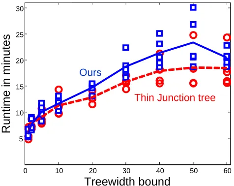
In this section we perform experimental validation of our approach and show that it is beneficial for learning Bayesian networks of bounded treewidth. Specifically, we demonstrate that by making use of global structure modification steps, our approach leads to superior generalization. In order to evaluate our method we compare against two strong baseline approaches.

The first baseline is an improved variant of the thin junction tree approach of Bach and Jordan (2002). We start, as in our method, with a Chow-Liu forest and iteratively add the single best scoring edge. To make the approach as comparable to ours as possible, at each iteration, we triangulate the model using either the maximum cardinality search or minimum fill-in heuristics (see, for example, Koster et al., 2001), as well as using our treewidth friendly triangulation, and take the triangulation that results in a lower treewidth.5 As in our method, when the treewidth bound is reached, we continue to add edges that improve the model selection score until no such edges can be found that do not also increase the treewidth bound.

The second baseline is an aggressive structure learning approach that combines greedy edge modifications with a TABU list (e.g., Glover and Laguna, 1993) and random moves. This approach is not constrained by a treewidth bound. Comparison to this baseline allows us to evaluate the merit of our method with respect to an unconstrained state-of-the-art search procedure.

We evaluate our method on four real-world data sets that are described below. Where relevant we also compare our results to the results of Chechetka and Guestrin (2008).

8.1 Gene Expression

In our first experiment, we consider a continuous data set based on a study that measures the expres-sion of the baker’s yeast genes in 173 experiments (Gasch et al., 2000). In this study, researchers measured the expression of 6152 yeast genes in response to changes in the environmental condi-tions, resulting in a matrix of 173×6152 measurements. The measurements are real-valued and, in our experiments, we learn sigmoid Bayesian networks using the Bayesian Information Criterion (BIC) (Schwarz, 1978) for model selection. For practical reasons, we consider the fully observed set of 89 genes that participate in general metabolic processes (Met). This is the larger of the two sets used by Elidan et al. (2007), and was chosen since part of the response of the yeast to changes in its environment is in altering the activity levels of different parts of its metabolism. We treat the genes as variables and the experiments as instances so that the learned networks indicate possible regulatory or functional connections between genes (Friedman et al., 2000).

Figure 8 shows test log-loss results for the 89 variable gene expression data set as a function of the treewidth bound. The first obvious phenomenon is that both our method (solid blue squares) and

5 10 15 20 25 30 35 40 45 50 55 60

-5 -4 -3 -2 -1 0 1

T

e

s

t

lo

g

-l

o

s

s

/

i

n

s

ta

n

c

e

Treewidth bound

Ours

Thin Junction-tree

Aggressive

Figure 8: Average test set log-loss per instance over five folds (y-axis) versus the treewidth bound (x-axis) for the 89 variable gene expression data set. Compared are our method (solid blue squares) with the Thin junction tree approach (dashed red circles), and an Aggressive greedy approach of unbounded treewidth that also uses a TABU list and random moves (dotted black).

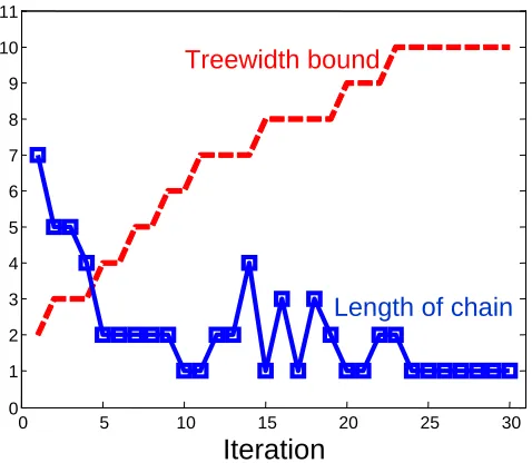
0 5 10 15 20 25 30

0 1 2 3 4 5 6 7 8 9 10 11

Iteration

Treewidth bound

Length of chain