Model Selection Through Sparse Maximum Likelihood Estimation
for Multivariate Gaussian or Binary Data
Onureena Banerjee [email protected]
Laurent El Ghaoui [email protected]
EECS Department
University of California, Berkeley Berkeley, CA 94720 USA
Alexandre d’Aspremont [email protected]
ORFE Department Princeton University Princeton, NJ 08544 USA
Editor: John Lafferty
Abstract
We consider the problem of estimating the parameters of a Gaussian or binary distribution in such a way that the resulting undirected graphical model is sparse. Our approach is to solve a maximum likelihood problem with an added`1-norm penalty term. The problem as formulated is convex but the memory requirements and complexity of existing interior point methods are prohibitive for problems with more than tens of nodes. We present two new algorithms for solving problems with at least a thousand nodes in the Gaussian case. Our first algorithm uses block coordinate descent, and can be interpreted as recursive`1-norm penalized regression. Our second algorithm, based on Nesterov’s first order method, yields a complexity estimate with a better dependence on problem size than existing interior point methods. Using a log determinant relaxation of the log partition function (Wainwright and Jordan, 2006), we show that these same algorithms can be used to solve an approximate sparse maximum likelihood problem for the binary case. We test our algorithms on synthetic data, as well as on gene expression and senate voting records data.
Keywords: model selection, maximum likelihood estimation, convex optimization, Gaussian graphical model, binary data
1. Introduction
Undirected graphical models offer a way to describe and explain the relationships among a set of variables, a central element of multivariate data analysis. The principle of parsimony dictates that we should select the simplest graphical model that adequately explains the data. In this paper we consider practical ways of implementing the following approach to finding such a model: given a set of data, we solve a maximum likelihood problem with an added`1-norm penalty to make the resulting graph as sparse as possible.
a gradient descent algorithm in which they account for the sparsity of the inverse covariance matrix by defining a loss function that is the negative of the log likelihood function. Speed and Kiiveri (1986) and, more recently, Dahl et al. (Revised 2007) proposed a set of large scale methods for problems where a sparsity pattern for the inverse covariance is given and one must estimate the nonzero elements of the matrix.
Another way to estimate the graphical model is to find the set of neighbors of each node in the graph by regressing that variable against the remaining variables. In this vein, Dobra and West (2004) employ a stochastic algorithm to manage tens of thousands of variables. There has also been a great deal of interest in using `1-norm penalties in statistical applications. d’Aspremont et al. (2004) apply an `1 norm penalty to sparse principle component analysis. Directly related to our problem is the use of the Lasso of Tibshirani (1996) to obtain a very short list of neighbors for each node in the graph. Meinshausen and B ¨uhlmann (2006) study this approach in detail, and show that the resulting estimator is consistent, even for high-dimensional graphs. A related approach is the graphical lasso, explored by Friedman et al. (2007).
Our objective here is to both estimate the sparsity pattern of the underlying graph and to obtain a regularized estimate of the covariance matrix. The difficulty of the problem formulation we consider lies in its computation. Although the problem is convex, it is non-smooth and has an unbounded constraint set. As we shall see, the resulting complexity for existing interior point methods is
O
(p6), where p is the number of variables in the distribution. In addition, interior point methods require that at each step we compute and store a Hessian of sizeO
(p2). The memory requirements and complexity are thus prohibitive forO
(p)higher than the tens. Specialized algorithms are needed to handle larger problems.The remainder of the paper is organized as follows. We begin by considering Gaussian data. In Section 2 we set up the problem, derive its dual, discuss properties of the solution and how heavily to weight the`1-norm penalty in our problem. In Section 3 we present a provably convergent block coordinate descent algorithm that can be interpreted a sequence of iterative`1-norm penalized regressions. In Section 4 we present a second, alternative algorithm based on Nesterov’s recent work on non-smooth optimization, and give a rigorous complexity analysis with better dependence on problem size than interior point methods. In Section 5 we show that the algorithms we developed for the Gaussian case can also be used to solve an approximate sparse maximum likelihood problem for multivariate binary data, using a log determinant relaxation for the log partition function given by Wainwright and Jordan (2006). In Section 6, we test our methods on synthetic as well as gene expression and senate voting records data.
2. Problem Formulation
In this section we set up the sparse maximum likelihood problem for Gaussian data, derive its dual, and discuss some of its properties.
2.1 Problem Setup
Suppose we are given n samples independently drawn from a p-variate Gaussian distribution:
y(1), . . . ,y(n)∼
N
(µ,Σp), where the covariance matrixΣis to be estimated. Let S denote the secondS :=1
n
n
∑
k=1
(y(k)−µ)(y(k)−µ)T.
Let ˆΣ−1denote our estimate of the inverse covariance matrix. Our estimator takes the form: ˆ
Σ−1=arg max
X0log det X−trace(SX)−λkXk1. (1) Here,kXk1denotes the sum of the absolute values of the elements of the positive definite matrix X . The scalar parameter λcontrols the size of the penalty. The penalty term is a proxy for the number of nonzero elements in X , and is often used—albeit with vector, not matrix, variables—in regression techniques, such as the Lasso.
In the case where S0, the classical maximum likelihood estimate is recovered for λ=0. However, when the number of samples n is small compared to the number of variables p, the sec-ond moment matrix may not be invertible. In such cases, forλ>0, our estimator performs some regularization so that our estimate ˆΣis always invertible, no matter how small the ratio of samples to variables is.
Even in cases where we have enough samples so that S0, the inverse S−1may not be sparse, even if there are many conditional independencies among the variables in the distribution. By trading off maximality of the log likelihood for sparsity, we hope to find a very sparse solution that still adequately explains the data. A larger value ofλcorresponds to a sparser solution that fits the data less well. A smallerλcorresponds to a solution that fits the data well but is less sparse. The choice ofλis therefore an important issue that will be examined in detail in Section 2.3.
2.2 The Dual Problem and Bounds on the Solution By expressing the`1norm in (1) as
kXk1= max
kUk∞≤1trace(XU),
wherekUk∞denotes the maximum absolute value element of the symmetric matrix U , we can write (1) as
max
X0kUmink∞≤λlog det X−trace(X,S+U).
This corresponds to seeking an estimate with the maximum worst-case log likelihood, over all additive perturbations of the second moment matrix S. A similar robustness interpretation can be made for a number of estimation problems, such as support vector machines for classification.
We can obtain the dual problem by exchanging the max and the min. The resulting inner prob-lem in X can be solved analytically by setting the gradient of the objective to zero and solving for X . The result is
min
kUk∞≤λ−log det(S+U)−p
where the primal and dual variables are related as: X = (S+U)−1. Note that the log determinant function acts a log barrier, creating an implicit constraint that S+U0.
To write things neatly, let W=S+U . Then the dual of our sparse maximum likelihood problem is
ˆ
Observe that the dual problem (2) estimates the covariance matrix while the primal problem esti-mates its inverse. We also observe that the diagonal elements of the solution areΣkk=Skk+λfor
all k.
The following theorem shows that adding the`1-norm penalty regularizes the solution. Theorem 1 For everyλ>0, the optimal solution to (1) is unique, with bounded eigenvalues:
p
λ ≥ kΣˆ−1k2≥(kSk2+λp)−1.
Here,kAk2 denotes the maximum eigenvalue of a symmetric matrix A. The proof is contained in the appendix.
The dual problem (2) is smooth and convex, albeit with p(p+1)/2 variables. For small values of p, the problem can be solved by existing interior point methods (e.g., Vandenberghe et al., 1998). The complexity to compute anε-suboptimal solution using such second-order methods, however, is
O
(p6log(1/ε)), making them infeasible when p is larger than the tens.A related problem, solved by Dahl et al. (Revised 2007), is to compute a maximum likelihood estimate of the covariance matrix when the sparsity structure of the inverse is known in advance. This is accomplished by adding constraints to (1) of the form: Xi j =0 for all pairs(i,j)in some
specified set. Our constraint set is unbounded as we hope to uncover the sparsity structure automat-ically, starting with a dense second moment matrix S.
2.3 Choice of Penalty Parameter
Consider the true, unknown graphical model for a given distribution. This graph has p nodes, and an edge between nodes k and j is missing if variables k and j are independent conditional on the rest of the variables. For a given node k, let Ck denote its connectivity component: the set of all
nodes that are connected to node k through some chain of edges. In particular, if node j6∈Ck, then
variables j and k are independent.
Meinshausen and B ¨uhlmann (2006) show that the Lasso, when used to estimate the set of neigh-bors for each node, yields an estimate of the sparsity pattern of the graph in a way that is asymp-totically consistent. Consistency, they show, hinges on the choice of the regularization parameter. In addition to asymptotic results, they prove a finite sample result: by choosing the regularization parameter in a particular way, the probability that two distinct connectivity components are falsely joined in the estimated graph can be controlled.
Following the methods used by Meinshausen and B ¨uhlmann (2006), we can derive a corre-sponding choice for the regularization parameter. Let ˆCλk denote our estimate of the connectivity component of node k. In the context of our optimization problem, this corresponds to the entries of row k in ˆΣthat are nonzero.
Letαbe a given level in[0,1]. Consider the following choice for the penalty parameter in (1):
λ(α):= (max
i>j σˆiσˆj)
tn−2(α/2p2)
q
n−2+tn2−2(α/2p2)
(3)
Theorem 2 Usingλ(α)the penalty parameter in (1), for any fixed levelα, P(∃k∈ {1, . . . ,p}: ˆCλk 6⊆Ck)≤α.
Observe that, for a fixed problem size p, as the number of samples n increases to infinity, the penalty parameterλ(α)decreases to zero. Thus, asymptotically we recover the classical maximum likelihood estimate, S, which in turn converges in probability to the true covarianceΣ.
Meinshausen and B ¨uhlmann (2006) prove that Lasso recovers the underlying sparsity pattern consistently, in a scheme where the number of variables is allowed to grow with the number of samples: p∈
O
(nγ). Although such an analysis is beyond the scope of this paper, a similar result seems to hold here provided we assume certain conditions on the true covariance matrix.From the point of view of estimating the covariance matrix itself, when the number of variables is allowed to grow with the number of samples, it may be better to use estimates such as those described by Bickel and Levina (2008), which are shown to be consistent in the operator norm as long as(log p)2/n→0.
3. Block Coordinate Descent Algorithm
In this section we present an algorithm for solving (2) that uses block coordinate descent.
3.1 Algorithm Description
We begin by detailing the algorithm. For any symmetric matrix A, let A\k\j denote the matrix
produced by removing column k and row j. Let Aj denote column j with the diagonal element Aj j
removed. The plan is to optimize over one row and column of the variable matrix W at a time, and to repeatedly sweep through all columns until we achieve convergence.
Initialize: W(0):=S+λI For k≥0
1. For j=1, . . . ,p
(a) Let W(j−1)denote the current iterate. Solve the quadratic program ˆ
y :=arg min
y {y
T(W(j−1)
\j\j )−
1y :ky−S
jk∞≤λ}. (4)
(b) Update rule: W(j)is W(j−1)with column/row Wj replaced by ˆy.
2. Let ˆW(0):=W(p).
3. After each sweep through all columns, check the convergence condition. Convergence occurs when
trace((Wˆ(0))−1S)
3.2 Convergence and Property of Solution
Using Schur complements, we can prove convergence:
Theorem 3 The block coordinate descent algorithm described above converges, achieving anε -suboptimal solution to (2). In particular, the iterates produced by the algorithm are strictly positive
definite: each time we sweep through the columns, W(j)0 for all j.
The proof of Theorem 3 sheds some interesting light on the solution to problem (1). In particular, we can use this method to show that the solution has the following property:
Theorem 4 Fix any k∈ {1, . . . ,p}. Ifλ≥ |Sk j|for all j6=k, then column and row k of the solution
ˆ
Σto (2) are zero, excluding the diagonal element.
This means that, for a given second moment matrix S, if λis chosen such that the condition in Theorem 4 is met for some column k, then the sparse maximum likelihood method estimates variable k to be independent of all other variables in the distribution. In particular, Theorem 4 implies that if
λ≥ |Sk j|for all k> j, then (1) estimates all variables in the distribution to be pairwise independent.
Using the work of Luo and Tseng (1992), it may be possible to show that the local convergence rate of this method is at least linear. In practice we have found that a small number of sweeps through all columns, independent of problem size p, is sufficient to achieve convergence. In each iteration, we must solve one quadratic program (QP). In a standard primal-dual interior point method for solving QPs, the computational cost is dominated by the cost of finding a search direction, which involves inverting matrices of size p. The cost of each iteration is therefore O(p3). For a fixed number of K sweeps, the cost of the method is O(K p4).
3.3 Interpretation as Iterative Penalized Regression The dual of (4) is
min
x x
TW(j−1)
\j\j x−S T
jx+λkxk1. (5)
Strong duality obtains so that problems (5) and (4) are equivalent. If we let Q denote the square root of W\(jj\−j1), and b :=1
2Q− 1S
j, then we can write (5) as
min
x kQx−bk
2
2+λkxk1. (6)
4. Nesterov’s First Order Method
In this section we apply the recent results due to Nesterov (2005) to obtain a first order algorithm for solving (1) with lower memory requirements and a rigorous complexity estimate with a better dependence on problem size than those offered by interior point methods. Our purpose is not to ob-tain another algorithm, as we have found that the block coordinate descent is fairly efficient; rather, we seek to use Nesterov’s formalism to derive a rigorous complexity estimate for the problem, im-proved over that offered by interior-point methods. In particular, although we have found in practice that a small, fixed number K of sweeps through all columns is sufficient to achieve convergence us-ing the block coordinate descent method, we have not been able to compute a bound on K. In what follows, we compute a guaranteed theoretical upper bound on the complexity of solving (1).
As we will see, Nesterov’s framework allows us to obtain an algorithm that has a complexity of O(p4.5/ε), whereε>0 is the desired accuracy on the objective of problem (1). This is in contrast to the complexity of interior-point methods, O(p6log(1/ε)). Thus, Nesterov’s method provides a much better dependence on problem size and lower memory requirements at the expense of a degraded dependence on accuracy.
4.1 Idea of Nesterov’s Method
Nesterov’s method applies to a class of non-smooth, convex optimization problems of the form
min
x {f(x): x∈Q1} (7)
where the objective function can be written as
f(x) = fˆ(x) +max
u {hAx,ui2: u∈Q2}.
Here, Q1 and Q2 are bounded, closed, convex sets, ˆf(x) is differentiable (with a Lipschitz-continuous gradient) and convex on Q1, and A is a linear operator. The challenge is to write our problem in the appropriate form and choose associated functions and parameters in such a way as to obtain the best possible complexity estimate, by applying general results obtained by Nesterov (2005).
Observe that we can write (1) in the form (7) if we impose bounds on the eigenvalues of the solution, X . To this end, we let
Q1:={x : aIXbI},
Q2:={u :kuk∞≤λ}
where the constants a,b are given such that b>a>0. By Theorem 1, we know that such bounds always exist. We also define ˆf(x):=−log det x+hS,xi, and A :=I.
To Q1 and Q2, we associate norms and continuous, strongly convex functions, called prox-functions, d1(x) and d2(u). For Q1 we choose the Frobenius norm, and a prox-function d1(x) = −log det x+p log b. For Q2, we choose the Frobenius norm again, and a prox-function d2(x) = kuk2F/2.
The method applies a smoothing technique to the non-smooth problem (7), which replaces the objective of the original problem, f(x), by a penalized function involving the prox-function d2(u):
˜
f(x) =fˆ(x) +max
The above function turns out to be a smooth uniform approximation to f everywhere. It is differentiable, convex on Q1, and a has a Lipschitz-continuous gradient, with a constant L that can be computed as detailed below. A specific gradient scheme is then applied to this smooth approximation, with convergence rate O(L/ε).
4.2 Algorithm and Complexity Estimate
To detail the algorithm and compute the complexity, we must first calculate some parameters cor-responding to our definitions and choices above. First, the strong convexity parameter for d1(x)on Q1isσ1=1/b2, in the sense that
∇2d1(X)[H,H] =trace(X−1HX−1H)
≥b−2kHk2F
for every symmetric H. Furthermore, the center of the set Q1 is x0:=arg minx∈Q1d1(x) =bI,
and satisfies d1(x0) =0. With our choice, we have D1:=maxx∈Q1 d1(x) =p log(b/a).
Similarly, the strong convexity parameter for d2(u)on Q2isσ2:=1, and we have
D2:=max
u∈Q2d2(U) =p
2/2.
With this choice, the center of the set Q2is u0:=arg minu∈Q2d2(u) =0.
For a desired accuracy ε, we set the smoothness parameter µ :=ε/2D2, and set x0=bI. The algorithm proceeds as follows:
For k≥0 do
1. Compute∇f˜(xk) =−x−1+S+u∗(xk), where u∗(x)solves (8).
2. Find yk=arg miny{h∇f˜(xk),y−xki+12L(ε)ky−xkk2F : y∈Q1}. 3. Find zk=arg minx{Lσ(ε)
1 d1(X) +∑ k
i=0i+21h∇f˜(xi),x−xii : x∈Q1}. 4. Update xk= k+23zk+kk++13yk.
In our case, the Lipschitz constant for the gradient of our smooth approximation to the objective function is
L(ε):=M+D2kAk2/(2σ2ε)
where M :=1/a2 is the Lipschitz constant for the gradient of ˜f , and the normkAkis induced by the Frobenius norm, and is equal toλ.
The algorithm is guaranteed to produce an ε-suboptimal solution after a number of steps not exceeding
N(ε):=
4kAk
r
D1D2
σ1σ2 · 1
ε+ q
MD1 σ1ε
= (κp(logκ))(4p1.5aλ/√2+√εp)/ε.
(9)
whereκ=b/a is a bound on the condition number of the solution.
amounts to projecting on Q1, and requires that we solve an eigenvalue problem. The same is true for Step 3. In fact, each iteration costs O(p3). The number of iterations necessary to achieve an objective with absolute accuracy less than ε is given in (9) by N(ε) =O(p1.5/ε). Thus, if the condition numberκis fixed in advance, the complexity of the algorithm is O(p4.5/ε).
5. Binary Variables: Approximate Sparse Maximum Likelihood Estimation
In this section, we consider the problem of estimating an undirected graphical model for multi-variate binary data. Recently, Wainwright et al. (2006) applied an`1-norm penalty to the logistic regression problem to obtain a binary version of the high-dimensional consistency results of Mein-shausen and B ¨uhlmann (2006). We apply the log determinant relaxation of Wainwright and Jordan (2006) to formulate an approximate sparse maximum likelihood (ASML) problem for estimating the parameters in a multivariate binary distribution. We show that the resulting problem is the same as the Gaussian sparse maximum likelihood (SML) problem, and that we can therefore apply our previously-developed algorithms to sparse model selection in a binary setting.
Consider a distribution made up of p binary random variables. Using n data samples, we wish to estimate the structure of the distribution. An Ising model for this distribution is
p(x;θ) =exp{
p
∑
i=1
θixi+ p−1
∑
i=1
p
∑
j=i+1
θi jxixj−A(θ)} (10)
where
A(θ) =log
∑
x∈Xp
exp{
p
∑
i=1
θixi+ p−1
∑
i=1
p
∑
j=i+1
θi jxixj} (11)
is the log partition function.
The sparse maximum likelihood problem in this case is to maximize (10) with an added`1-norm penalty on termsθk j. Specifically, in the undirected graphical model, an edge between nodes k and
j is missing ifθk j=0.
A well-known difficulty is that the log partition function has too many terms in its outer sum to compute. However, if we use the log determinant relaxation for the log partition function devel-oped by Wainwright and Jordan (2006), we can obtain an approximate sparse maximum likelihood (ASML) estimate.
5.1 Problem Formulation
Let’s begin with some notation. Letting d :=p(p+1)/2, define the map R : Rd→Sp+1as follows:
R(θ) =
0 θ1 θ2 . . . θp
θ1 0 θ12 . . . θ1p
.. .
θp θ1p θ2p . . . 0
Suppose that our n samples are z(1), . . . ,z(n)∈ {−1,+1}p. Let ¯zi and ¯zi j denote sample mean
and second moments. The sparse maximum likelihood problem is
ˆ
θexact :=arg max
θ
1
2hR(θ),R(¯z)i −A(θ)−λkθk1. (12) Finally define the constant vector m= (1,4
3, . . . , 4
3)∈Rp+1. Wainwright and Jordan (2006) give an upper bound on the log partition function as the solution to the following variational problem:
A(θ)≤maxµ12log det(R(µ) +diag(m)) +hθ,µi =12·maxµlog det(R(µ) +diag(m)) +hR(θ),R(µ)i.
(13)
If we use the bound (13) in our sparse maximum likelihood problem (12), we won’t be able to extract an optimizing argument ˆθ. Our first step, therefore, will be to rewrite the bound in a form that will allow this.
Lemma 5 We can rewrite the bound (13) as
A(θ)≤ p
2log(
eπ
2 )− 1
2(p+1)− 1
2· {maxν ν
Tm+log det(−(R(θ) +diag(ν))). (14)
Using this version of the bound (13), we have the following theorem.
Theorem 6 Using the upper bound on the log partition function given in (14), the approximate sparse maximum likelihood problem has the following solution:
ˆ
θk=¯µk
ˆ
θk j=−(Γˆ)−k j1
(15)
where the matrix ˆΓis the solution to the following problem, related to (2):
ˆ
Γ:=arg max{log detW : Wkk=Skk+
1
3,|Wk j−Sk j| ≤λ}. (16)
Here, S is defined as before:
S=1
n
n
∑
k=1
(z(k)−¯µ)(z(k)−¯µ)T
where ¯µ is the vector of sample means ¯zi.
5.2 Penalty Parameter Choice for Binary Variables
For the choice of the penalty parameterλ, we can derive a formula analogous to (3). Consider the choice
λ(α)bin := (χ
2(α/2p2,1))1 2
(mini>jσˆiσˆj)√n
(17)
whereχ2(α,1) is the (100−α)% point of the chi-square distribution for one degree of freedom. Since our variables take on values in{−1,1}, the empirical variances are of the form:
ˆ
σ2
i =1−¯µ2i.
Using (17), we have the following binary version of Theorem 2:
Theorem 7 With (17) chosen as the penalty parameter in the approximate sparse maximum
likeli-hood problem, for a fixed levelα,
P(∃k∈ {1, . . . ,p}: ˆCλk 6⊆Ck)≤α.
6. Numerical Results
In this section we present the results of some numerical experiments, both on synthetic and real data. The synthetic experiments were performed on continuous data, and tests only the original problem formulation. Both continuous and discrete real data sets are used, however, testing the Gaussian and binary formulations respectively.
6.1 Synthetic Experiments
Synthetic experiments require that we generate underlying sparse inverse covariance matrices. To this end, we first randomly choose a diagonal matrix with positive diagonal entries. A given number of nonzeros are inserted in the matrix at random locations symmetrically. Positive definiteness is ensured by adding a multiple of the identity to the matrix if needed. The multiple is chosen to be only as large as necessary for inversion with no errors.
6.2 Sparsity and Thresholding
A very simple approach to obtaining a sparse estimate of the inverse covariance matrix would be to apply a threshold to the inverse empirical covariance matrix, S−1. However, even when S is easily invertible, it can be difficult to select a threshold level. We solved a synthetic problem of size p=100 where the true concentration matrix density was set toδ=0.1. Drawing n=200 samples, we plot in Figure 1 the sorted absolute value elements of S−1on the left and ˆΣ−1, the solution to (1), on the right.
It is clearly easier to choose a threshold level for the sparse maximum likelihood estimate. Applying a threshold to either S−1 or ˆΣ−1 would decrease the log likelihood of the estimate by an unknown amount. One way to compute the largest possible threshold t that preserves positive definiteness in S can be computed by solving the minimization problem:
t≤ min
kvk1=1
The condition (6.2) is equivalent to the condition that S−1+L0 for all matrices L such that
kLk∞≤t.
0 2000 4000 6000 8000 10000
0 2 4 6 8 10
(A)
0 2000 4000 6000 8000 10000
0 2 4 6 8 10
(B)
Figure 1: Sorted absolute value of elements of (A) S−1 and (B) ˆΣ−1. The solution ˆΣ−1 to (1) is un-thresholded.
6.3 Recovering Structure
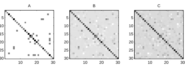
We begin with a small experiment to test the ability of the method to recover the sparse structure of an underlying covariance matrix. Figure 2 (A) shows a sparse inverse covariance matrix of size p=30. Figure 2 (B) displays a corresponding S−1, using n=60 samples. Figure 2 (C) displays the solution to (1) forλ=0.1. The value of the penalty parameter here is chosen arbitrarily, and the solution is not thresholded. Nevertheless, we can still pick out features that were present in the true underlying inverse covariance matrix.
A
10 20 30 5
10 15 20 25 30
B
10 20 30 5
10 15 20 25 30
C
10 20 30 5
10 15 20 25 30
A
10 20 30 5
10 15 20 25 30
B
10 20 30 5
10 15 20 25 30
C
10 20 30 5
10 15 20 25 30
Figure 3: Recovering the sparsity pattern for small sample size. We plot (A) the original inverse covariance matrixΣ−1, (B) the solution to problem (1) for n=30 and (C) the solution for n=20. A penalty parameter ofλ=0.1 is used for (B) and (C).
6.4 CPU Times Versus Problem Size
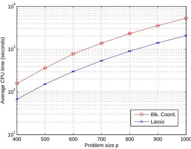
For a sense of the practical performance of the block coordinate descent method, we implemented it in Matlab, using Mosek to solve the quadratic program at each step. For problem sizes ranging from p=400 to p=1000, we solved the problem using n=2p samples. In all cases, one sweep through all the columns was sufficient to achieve an absolute accuracy ofε=1e−7. The Nesterov algorithm, implemented in C, was found to have a comparable computation time provided one chooses a large value for the desired accuracy. Since the Nesterov algorithm aims for a lower accuracy and requires the setting of bounds a and b on the eigenvalues of the solution, it was not included in this experiment.
In Figure 4 we plot the average CPU time to achieve convergence, along with CPU times for the Lasso for comparision. CPU times were computed using an AMD Athlon 64 2.20Ghz processor with 1.96GB of RAM. Using this very simple implementation, the block coordinate descent method solves a problem of size p=1000 in about an hour and a half. The computation time could possibly be cut down by using a fast Lasso implementation to solve the optimization problem, as described in Section 3.3, and by using a suitable method to compute the square root matrix Q from (6).
6.5 Path Following Experiments
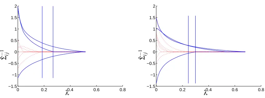
Figure 6.5 shows two path following examples. We solve two randomly generated problems of size p=5 and n=100 samples. The red lines correspond to elements of the solution that are zero in the true underlying inverse covariance matrix. The blue lines correspond to true nonzeros. The vertical lines mark ranges ofλfor which we recover the correct sparsity pattern exactly. Note that, by Theorem 4, forλvalues greater than those shown, the solution will be diagonal.
On a related note, we observe that (1) also works well in recovering the sparsity pattern of a matrix masked by noise. The following experiment illustrates this observation. We generate a sparse inverse covariance matrix of size p=50 as described above. Then, instead of using an empirical covariance S as input to (1), we use S= (Σ−1+V)−1, where V is a randomly generated uniform noise of sizeσ=0.1. We then solve (1) for various values of the penalty parameterλ.
400 500 600 700 800 900 1000 101
102 103 104
Problem size p
Average CPU time (seconds)
Blk. Coord. Lasso
Figure 4: Average CPU times vs. problem size using block coordinate descent. We plot the average CPU time (in seconds) versus problem size. The standard deviations for the block coor-dinate descent method are: 0.6077, 0.2652, 0.1989, 1.0165, 48.0833, 2.7732, and 6.2314 seconds respectively. For the Lasso, the standard deviations are: 0.0221, 0.3646, 0.1878, 0.5966, 12.7279, 13.1257, and 0.6187 seconds respectively.
to (1). We plot the average percentage of errors (number of misclassified zeros plus misclassified nonzeros divided by p2), as well as error bars corresponding to one standard deviation. As shown, the error rate is nearly zero on average when the penalty is set to equal the noise levelσ.
6.6 Estimating the Stability of the Solution Using Cross-validation
Viewing our estimator as a machine that classifies elements of the concentration matrix as either zero or nonzero, we next turn to the question of the stability of the classification. Classifier instability is defined here as the probability that the classification of an arbitrary element of the matrix is changed by some small disturbance in the data. In other words, once we obtain a concentration graph by treating our estimated matrix ˆΣ as an adjacency matrix, we would like to measure the stability of our results.
0 0.2 0.4 0.6 0.8 −1.5
−1 −0.5 0 0.5 1 1.5 2
PSfrag replacements
ˆΣ
−
1
ij
λ −1.50 0.2 0.4 0.6 0.8
−1 −0.5 0 0.5 1 1.5 2
PSfrag replacements ˆ
Σ−1
i j λ
λ
ˆΣ
−
1
ij
Figure 5: Path following: elements of solution to (1) asλincreases. Dashed lines correspond to elements that are zero in the true inverse covariance matrix; solid lines correspond to true nonzeros. Vertical lines mark a range ofλ values using which we recover the sparsity pattern exactly.
−0.50 0 0.5 1 1
2 3 4 5 6 7
PSfrag replacements
Error
(in
%)
log(λ/σ)
Figure 6: Recovering sparsity pattern in a matrix with added uniform noise of size σ=0.1. We plot the average percentage or misclassified entries as a function of log(λ/σ).
0 2 4 6 8 10 12 14 −0.01
−0.005 0 0.005 0.01 0.015 0.02 0.025
n = 30 n = 60 n = 100
PSfrag replacements
λ
Estimated
Instability
Figure 7: Estimating stability of the solution using cross validation. We plot estimated instability, the probability that the classification of an arbitrary element is changed by a small distur-bance in the data, for a range of values ofλusing data sets of size n=30,60, and 100 samples for a problem with p=30 variables.
Below we show the results of some experiments using synthetic data. First, we randomly gener-ated an underlying concentration matrix of size p=30. Letδ=0.25 denote the fraction of nonzero elements inΣ−1. Then, from the corresponding covariance matrixΣ, we generated three data sets of sizes n=30,60, and 100.
In Figure 7 we plot estimated instability versus a range of values for the penalty parameterλ, using 10-fold cross validation. We applied Theorem 4 to compute a maximum value ofλ; beyond this value, the estimated graph is empty for all three data sets. As shown, even for a small number of samples, the estimated graph is fairly stable for all values ofλ.
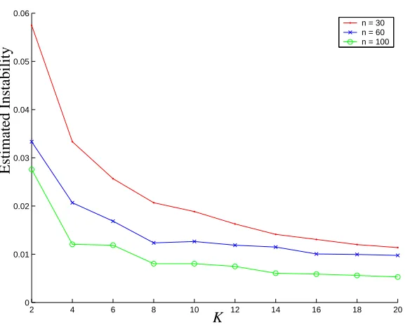
We can also see how our estimate of the instability changes as we divide the available data into a greater number of subsamples. In Figure 8 we repeat the experiment described above, this time fixingλ=0.2 and instead varying the number of folds K in the cross validation. In these examples, for each value of n, dividing the available data into more subsamples for cross validation decreases our estimate of the instability.
6.7 Performance as a Binary Classifier
2 4 6 8 10 12 14 16 18 20 0
0.01 0.02 0.03 0.04 0.05 0.06
n = 30 n = 60 n = 100
PSfrag replacements
K
Estimated
Instability
Figure 8: Estimating instability of the solution using cross validation. We plot the estimate of the instability obtained using K samples, for various values of K. Once again, we use data sets of size n=30,60, and 100 samples for a problem with p=30 variables.
declaring an element ˆΣi jnonzero if bothθ(ik)=6 0 andθ(jk)6=0 (Lasso-AND) or, less conservatively,
if either of those quantities is nonzero (Lasso-OR).
As noted previously, Meinshausen and B ¨uhlmann (2006) have also derived a formula for choos-ing their penalty parameter. Both the SML and Lasso penalty parameter formulas depend on a chosen levelα, which is a bound on the same error probability for each method. For these experi-ments, we setα=0.05.
In the following experiments, we fixed the problem size p at 30 and generated sparse underlying inverse covariance matrices as described above. We varied the number of samples n from 10 to 310. For each value of n shown, we ran 30 trials in which we estimated the sparsity pattern of the inverse covariance matrix using the SML, Lasso-OR, and Lasso-AND methods. We then recorded the average number of nonzeros estimated by each method, and the average number of entries correctly identified as nonzero (true positives).
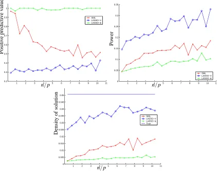
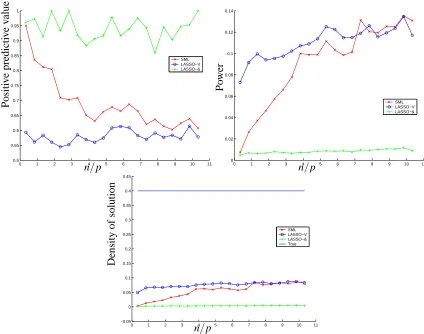
We show two sets of plots. Figure 6.7 corresponds to experiments where the true density was set to be low, δ=0.05. We plot the power (proportion of correctly identified nonzeros), positive predictive value (proportion of estimated nonzeros that are correct), and the density estimated by each method. Figure 6.7 corresponds to experiments where the true density was set to be high,
δ=0.40, and we plot the same three quantities.
1 2 3 4 5 6 7 8 9 10 11 0.2 0.3 0.4 0.5 0.6 0.7 0.8 0.9 1 SML LASSO−V LASSO−& PSfrag replacements Positi v e predicti v e v alue
n/p Power 0 1 2 3 4 5 6 7 8 9 10 11
0.05 0.1 0.15 0.2 0.25 0.3 0.35 SML LASSO−V LASSO−& PSfrag replacements Positive predictive value
n/p
Po
wer
1 2 3 4 5 6 7 8 9 10 11
0 0.005 0.01 0.015 0.02 0.025 0.03 0.035 0.04 0.045 0.05 SML LASSO−V LASSO−& True PSfrag replacements
n/p
Density
of
solution
Figure 9: Classifying zeros and nonzeros for a true density ofδ=0.05. We plot the positive predic-tive value, the power, and the estimated density using SML, Lasso-OR and Lasso-AND.
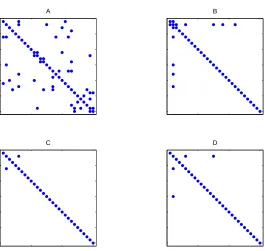
number of errors, tied with either Lasso-AND or Lasso-OR. Among the two Lasso methods, it would seem that if the true density is very low, it is slightly better to use the more conservative Lasso-AND. If the density is higher, it may be better to use Lasso-OR. When the true density is unknown, we can achieve an accuracy comparable to the better choice among the Lasso methods by computing the SML estimate. Figure 11 shows one example of sparsity pattern recovery when the true density is low.
The Lasso and SML methods have a comparable computational complexity. However, unlike the Lasso, the SML method is not parallelizable. Parallelization would render the Lasso a more computationally attractive choice, since each variable can regressed against all other separately, at an individual cost of
O
(p3). In exchange, SML can offer a more accurate estimate of the sparsity pattern, as well as a well-conditioned estimate of the covariance matrix itself.6.8 Recovering Structure from Binary Data
0 1 2 3 4 5 6 7 8 9 10 11 0.5 0.55 0.6 0.65 0.7 0.75 0.8 0.85 0.9 0.95 1 SML LASSO−V LASSO−& PSfrag replacements Positi v e predicti v e v alue
n/p Power 00 1 2 3 4 5 6 7 8 9 10 11
0.02 0.04 0.06 0.08 0.1 0.12 0.14 SML LASSO−V LASSO−& PSfrag replacements Positive predictive value
n/p
Po
wer
0 1 2 3 4 5 6 7 8 9 10 11
−0.05 0 0.05 0.1 0.15 0.2 0.25 0.3 0.35 0.4 0.45 SML LASSO−V LASSO−& True PSfrag replacements
n/p
Density
of
solution
Figure 10: Classifying zeros and nonzeros for a true density of δ=0.40. We plot the positive predictive value, the power, and the estimated density using SML, OR and Lasso-AND.
resulting graph was d=4. We drew n i.i.d. samples and then attempted to recover the underly-ing sparsity pattern usunderly-ing both the approximate sparse maximum likelihood method and `1-norm penalized logistic regression as described by Wainwright et al. (2006).
In Figure 12 we plot the average sensitivity (the fraction of actual nonzeros that are correctly identified as nonzeros) as well as the average specificity (the fraction of actual zeros that are cor-rectly identified as zeros) for a range of sample sizes. We used a significance level ofα=0.05 for the approximate sparse maximum likelihood method, and a regularization parameter choice of
λn=0.04∗(log p)3/√n for the penalized logistic regression AND method, as described by
Wain-wright et al. (2006).
7. Gene Expression and U.S. Senate Voting Records Data
A B
C D
Figure 11: Comparing sparsity pattern recovery to the Lasso. (A) true covariance (B) Lasso-OR (C) Lasso-AND (D) SML.
0 500 1000 1500 2000
0.1 0.2 0.3 0.4 0.5 0.6 0.7 0.8 0.9
PLR−AND SML
PSfrag replacements
Sensiti
vity
n 0 500 1000 1500 2000
0.96 0.965 0.97 0.975 0.98 0.985 0.99 0.995 1 1.005
PLR−AND SML
PSfrag replacements Sensitivity n
Specificity
n
Figure 12: Comparing sparsity pattern recovery to the`1-norm penalized logistic regression (PLR). We show the sensitivity (left) as well as the specificity (right) as the number of samples is increased.
7.1 Rosetta Inpharmatics Compendium
We applied our algorithms to the Rosetta Inpharmatics Compendium of gene expression profiles described by Hughes et al. (2000). The 300 experiment compendium contains n=253 samples with p=6136 variables. With a view towards obtaining a very sparse graph, we replacedα/2p2in (3) byα, and setα=0.05. The resulting penalty parameter isλ=0.0313.
This is a large penalty for this data set, and by applying Theorem 4 we find that all but 270 of the variables are estimated to be independent from all the rest, clearly a very conservative estimate. Figure 13 displays the resulting graph.
Figure 13: Application to Hughes compendium. The above graph results from solving (1) for this data set with a penalty parameter ofλ=0.0313.
Figure 14 focuses on a region of Figure 13, a cluster of genes that is unconnected to the remain-ing genes in this estimate. Accordremain-ing to Gene Ontology (see Ashburner et al., 2000), these genes are associated with iron homeostasis. The probability that a gene has been false included in this cluster is at most 0.05.
Figure 14: Application to Hughes data set (closeup of Figure 13). These genes are associated with iron homeostasis.
7.2 Iconix Microarray Data
Next we analyzed a subset of a 10,000 gene microarray data set from 160 drug treated rat livers (Natsoulis et al., 2005). In this study, rats were treated with a variety of fibrate, statin, or estro-gen receptor agonist compounds. Taking the 500 estro-genes with the highest variance, we once again replacedα/2p2in (3) byα, and setα=0.05. The resulting penalty parameter isλ=0.0853.
By applying Theorem 4 we find that all but 339 of the variables are estimated to be independent from the rest. This estimate is less conservative than that obtained in the Hughes case since the ratio of samples to variables is 160 to 500 instead of 253 to 6136.
The first order neighbors of any node in a Gaussian graphical model form the set of predictors for that variable. In the estimated obtained by solving (1), we found that LDL receptor had one of the largest number of first-order neighbors in the Gaussian graphical model. The LDL receptor is believed to be one of the key mediators of the effect of both statins and estrogenic compounds on LDL cholesterol. Table 1 lists some of the first order neighbors of LDL receptor.
Figure 15: Application to Hughes data set (subgraph of Figure 13). These genes are associated with cellular membrane fusion.
ACCESSION GENE
BF553500 CBP/P300-INTERACTING TRANSACTIVATOR
BF387347 EST
BF405996 CALCIUM CHANNEL,VOLTAGE DEPENDENT
NM 017158 CYTOCHROMEP450, 2C39
K03249 ENOYL-COA,HYDRATASE/3-HYDROXYACYLCOADEHYDROG.
BE100965 EST
AI411979 CARNITINEO-ACETYLTRANSFERASE AI410548 3-HYDROXYISOBUTYRYL-COAHYDROLASE NM 017288 SODIUM CHANNEL,VOLTAGE-GATED
Y00102 ESTROGEN RECEPTOR1
NM 013200 CARNITINE PALMITOYLTRANSFERASE1B
Table 1: Predictor genes for LDL receptor.
7.3 Senate Voting Records Data
Figure 16: US Senate, 109th Congress (2004-2006). The graph displays the solution to (12) ob-tained using the log determinant relaxation to the log partition function of Wainwright and Jordan (2006). Democratic senators are represented by round nodes and Republican senators are represented by square nodes.
Each of the 542 samples is bill that was put to a vote. The votes are recorded as -1 for no and 1 for yes.
There are many missing values in this data set, corresponding to missed votes. Since our analysis depends on data values taken solely from{−1,1}, it was necessary to impute values to these. For this experiment, we replaced all missing votes with noes (-1). We chose the penalty parameterλ(α)
according to (17), using a significance level ofα=0.05. Figure 16 shows the resulting graphical model, rendered using Cytoscape. Red nodes correspond to Republican senators, and blue nodes correspond to Democratic senators.
We can make some tentative observations by browsing the network of senators. As neighbors most Democrats have only other Democrats and Republicans have only other Republicans. Senator Chafee (R, RI) has only Democrats as his neighbors, an observation that supports media statements made by and about Chafee during those years. Senator Allen (R, VA) unites two otherwise separate groups of Republicans and also provides a connection to the large cluster of Democrats through Ben Nelson (D, NE), which also supports media statements made about him prior to his 2006 re-election campaign. Thus, although we obtained this graphical model via a relaxation of the log partition function, the resulting picture is supported by conventional wisdom. Figure 17 shows a subgraph consisting of neighbors of degree three or lower of Senator Allen.
Figure 17: US Senate, 109th Congress. Neighbors of Senator Allen (degree three or lower).
Acknowledgments
We are indebted to Georges Natsoulis for his interpretation of the Iconix data set analysis and for gathering the senate voting records. We also thank Martin Wainwright, Bin Yu, Peter Bartlett, and Michael Jordan for many enlightening conversations.
Appendix A. Proof of Solution Properties and Block Coordinate Descent Convergence
In this section, we give short proofs of the two theorems on properties of the solution to (1), as well as the convergence of the block coordinate descent method.
Proof of Theorem 1:
Since ˆΣsatisfies ˆΣ=S+U , whereˆ kUk∞≤λ, we have:
kΣˆk2=kS+Uˆk2
≤ kSk2+kUk2≤ kSk2+kUk∞≤ kSk2+λp
which yields the lower bound onkΣˆ−1k2. Likewise, we can show thatkΣˆ−1k2is bounded above. At the optimum, the primal dual gap is zero:
−log det ˆΣ−1+trace(S ˆΣ−1) +λkΣˆ−1k
1−log det ˆΣ−p
=trace(S ˆΣ−1) +λkΣˆ−1k
1−p=0 We therefore have
kΣˆ−1k
2≤ kΣˆ−1kF≤ kΣˆ−1k1
where the last inequality follows from trace(S ˆΣ−1)≥0, since S0 and ˆΣ−10.
Next we prove the convergence of block coordinate descent:
Proof of Theorem 3:
To see that optimizing over one row and column of W in (2) yields the quadratic program (4), let all but the last row and column of W be fixed. Since we know the diagonal entries of the solution, we can fix the remaining diagonal entry as well:
W=
W\p\p wp
wTp Wpp
.
Then, using Schur complements, we have that
detW=detW\p\p·(Wpp−wTp(W\p\p)−1wp)
which gives rise to (4).
By general results on block coordinate descent algorithms (e.g., Bertsekas, 1998), the algorithms converges if (4) has a unique solution at each iteration. Thus it suffices to show that, at every sweep, W(j)0 for all columns j. Prior to the first sweep, the initial value of the variable is positive definite: W(0)0 since W(0):=S+λI, and we have S0 andλ>0 by assumption.
Now suppose that W(j)0. This implies that the following Schur complement is positive:
wj j−WjT(W
(j)
\j\j)−
1W
j>0
By the update rule we have that the corresponding Schur complement for W(j+1)is even greater:
wj j−WjT(W
(j+1)
\j\j )−
1W
j>wj j−WjT(W
(j)
\j\j)−
1W
j>0
so that W(j+1)0.
Finally, we apply Theorem 3 to prove the second property of the solution.
Proof of Theorem 4:
Suppose that column j of the second moment matrix satisfies|Si j| ≤λfor all i6= j. This means
that the zero vector is in the constraint set of (4) for that column. Each time we return to column j, the objective function will be different, but always of the form yTAy for A0. Since the constraint set will not change, the solution for column j will always be zero. By Theorem 3, the block co-ordinate descent algorithm converges to a solution, and so therefore the solution must have ˆΣj=0.
Appendix B. Proof of Error Bounds
B.1 Preliminaries
Before we begin, consider problem (1), for a matrix S of any size:
ˆ
X=arg min−log det X+trace(SX) +λkXk1
where we have dropped the constraint X0 since it is implicit, due to the log determinant function. Since the problem is unconstrained, the solution ˆX must correspond to setting the subgradient of the objective to zero:
Si j−Xi j−1=−λ for Xi j>0,
Si j−Xi j−1=λ for Xi j<0,
|Si j−Xi j−1| ≤λ for Xi j=0.
(18)
Recall that by Theorem 1, the solution is unique forλpositive.
B.2 Proof of Error Bound for Gaussian Data Now we are ready to prove Theorem 2.
Proof of Theorem 2:
Sort columns of the covariance matrix so that variables in the same connectivity component are grouped together. The correct zero pattern for the covariance matrix is then block diagonal. Define
Σcorrect :=blk diag(C1, . . . ,C`) (19)
The inverse(Σcorrect)−1must also be block diagonal, with possible additional zeros inside the blocks. If we constrain the solution to (1) to have this structure, then by the form of the objective, we can optimize over each block separately. For each block, the solution is characterized by (18).
Now, suppose that
λ> max
i∈N,j∈N\Ci
|Si j−Σcorrecti j |. (20)
Then, by the subgradient characterization of the solution noted above, and the fact that the solution is unique forλ>0, it must be the case that ˆΣ=Σcorrect. By the definition ofΣcorrect, this implies
that, for ˆΣ, we have ˆCk=Ckfor all k∈N.
Taking the contrapositive of this statement, we can write:
P(∃k∈N : ˆCk6⊆Ck)
≤P(maxi∈N,j∈N\Ci|Si j−Σ
correct
i j | ≥λ)
≤p2(n)·maxi∈N,j∈N\CiP(|Si j−Σ
correct
i j | ≥λ)
=p2(n)·maxi∈N,j∈N\CiP(|Si j| ≥λ).
(21)
The equality at the end follows since, by definition, Σcorrecti j =0 for j∈N\Ci. It remains to
bound P(|Si j| ≥λ).
The statement|Sk j| ≥λcan be written as:
|Rk j|(1−R2k j)− 1
2 ≥λ(skksj j−λ2)− 1 2
where Rk jis the correlation between variables k and j, since
|Rk j|(1−R2k j)− 1
2 =|Sk j|(SkkSj j−S2 k j)−
Furthermore, the condition j∈N\Ckis equivalent to saying that variables k and j are
indepen-dent:Σk j=0. Conditional on this, the statistic
Rk j(1−R2k j)−
1 2(n−2)
1 2
has a Student’s t-distribution for n−2 degrees of freedom. Therefore, for all j∈N\Ck,
P(|Sk j| ≥λ|Skk=skk,Sj j=sj j)
=2P(Tn−2≥λ(skksj j−λ2)− 1
2(n−2)12|Skk=skk,Sj j=sj j)
≤2 ˜Fn−2(λ(σˆ2kσˆ2j−λ2)− 1 2(n−2)
1 2)
(22)
where ˆσ2k is the sample variance of variable k, and ˜Fn−2=1−Fn−2 is the CDF of the Student’s t-distribution with n−2 degree of freedom. This implies that, for all j∈N\Ck,
P(|Sk j| ≥λ)≤2 ˜Fn−2(λ(σˆ2kσˆ2j−λ2)−
1 2(n−2)
1 2)
since P(A) =R
P(A|B)P(B)dB≤KR
P(B)dB=K. Putting the inequalities together, we have that:
P(∃k : ˆCkλ6⊆Ck)
≤p2·maxk,j∈N\Ck2 ˜Fn−2(λ(σˆ 2
kσˆ2j−λ2)− 1 2(n−2)
1 2) =2p2F˜n−2(λ((n−2)/((maxi>jσˆkσˆj)2−λ2))
1 2).
For any fixedα, our required condition onλis therefore
˜
Fn−2(λ((n−2)/((max
i>j σˆkσˆj)
2
−λ2))12) =α/2p2
which is satisfied by choosingλaccording to (3).
B.3 Proof of Bound for Binary Data
We can reuse much of the previous proof to derive a corresponding formula for the binary case.
Proof of Theorem 7:
The proof of Theorem 7 is identical to the proof of Theorem 2, except that we have a different null distribution for|Sk j|. The null distribution of
nR2k j
is chi-squared with one degree of freedom. Analogous to (22), we have:
P(|Sk j| ≥λ|Skk=skk,Sj j=sj j)
=2P(nR2k j≥nλ2skksj j|Skk=skk,Sj j=sj j)
≤2 ˜G(nλ2σˆ2
kσˆ2j)
where ˆσ2k is the sample variance of variable k, and ˜G=1−G is the CDF of the chi-squared distri-bution with one degree of freedom. This implies that, for all j∈N\Ck,
P(|Sk j| ≥λ)≤2 ˜G((λσˆkσˆj
√
Putting the inequalities together, we have that:
P(∃k : ˆCkλ6⊆Ck)
≤p2·maxk,j∈N\Ck2 ˜G((λσˆkσˆj √
n)2)
=2p2G˜((mini>jσˆkσˆj)2nλ2)
so that, for any fixedα, we can achieve our desired bound by choosingλ(α)according to (17).
Appendix C. Proof of Connection Between Gaussian SML and Binary ASML
We end with a proof of Theorem 6, which connects the exact Gaussian sparse maximum likelihood problem with the approximate sparse maximum likelihood problem obtained by using the log de-terminant relaxation of Wainwright and Jordan (2006). First we must prove Lemma 5.
Proof of Lemma 5:
The conjugate function for the convex normalization A(θ)is defined as
A∗(µ):=sup
θ {hµ,θi −A(θ)}. (23)
Wainwright and Jordan derive a lower bound on this conjugate function using an entropy bound:
A∗(µ)≥B∗(µ). (24)
Since our original variables are spin variables x{−1,+1}, the bound given in the paper is
B∗(µ):=−1
2log det(R(µ) +diag(m))− p 2log(
eπ
2 ) (25)
where m := (1,43, . . . ,43).
The dual of this lower bound is B(θ):
B∗(µ):=maxθhθ,µi −B(θ)≤maxθhθ,µi −A(θ) =: A∗(µ). (26)
This means that, for all µ,θ,
hθ,µi −B(θ)≤A∗(µ) (27)
or
B(θ)≥ hθ,µi −A∗(µ) (28)
so that in particular
B(θ)≥max
µ hθ,µi −A
Using the definition of B(θ)and its dual B∗(µ), we can write
B(θ):=maxµhθ,µi −B∗(µ)
=2plog(e2π) +maxµ12hR(θ),R(µ)i+12log det(R(µ) +diag(m)) =2plog(eπ
2) + 1
2·max{hR(θ),X−diag(m)i+log det(X): X0,diag(X) =m}
=2plog(eπ
2) + 1
2· {maxX0minνhR(θ),X−diag(m)i+log det(X) +ν
T(diag(X)−m)} =2plog(eπ
2) + 1
2· {maxX0minνhR(θ) +diag(ν),Xi+log det(X)−νTm}
=2plog(eπ
2) + 1
2· {minν−ν
Tm+max
X0hR(θ) +diag(ν),Xi+log det(X)}
=2plog(e2π) +12· {minν−νTm−log det(−(R(θ) +diag(ν)))−(p+1)} =2plog(eπ
2)− 1
2(p+1) + 1
2· {minν−ν
Tm−log det(−(R(θ) +diag(ν)))}
=2plog(e2π)−12(p+1)−12· {maxννTm+log det(−(R(θ) +diag(νλ)}.
(30)
Now we use Lemma 5 to prove the main result of Section 5.1. Having expressed the upper bound on the log partition function as a constant minus a maximization problem will help when we formulate the sparse approximate maximum likelihood problem.
Proof of Theorem 6:
The approximate sparse maximum likelihood problem is obtained by replacing the log partition function A(θ)with its upper bound B(θ), as derived in Lemma 5:
n· {maxθ12hR(θ),R(¯z)i −B(θ)−λkθk1}
=n· {maxθ12hR(θ),R(¯z)i −λkθk1+12(p+1)−2plog(e2π)
+1
2· {maxννTm+log det(−(R(θ) +diag(ν)))}}
=n2(p+1)−np2 log(e2π) +n2·maxθ,ν{νTm+hR(θ),R(¯z)i +log det(−(R(θ) +diag(ν)))−2λkθk1}.
(31)
We can collect the variables θ and νinto an unconstrained symmetric matrix variable Y :=
−(R(θ) +diag(ν)). Observe that
hR(θ),R(¯z)i=h−Y−diag(ν),R(¯z)i
=−hY,R(¯z)i − hdiag(ν),R(¯z)i=−hY,R(¯z)i (32)
and that
νTm=hdiag(ν),diag(ν)i=h−Y−R(θ),diag(m)i
=−hY,diag(m)i − hR(θ),diag(m)i=−hY,diag(m)i. (33)
The approximate sparse maximum likelihood problem can then be written in terms of Y :
n
2(p+1)−
np
2 log(
eπ
2) +
n
2·maxθ,ν{ν
Tm+hR(θ),R(¯z)i +log det(−(R(θ) +diag(m)))−2λkθk1}
=n
2(p+1)−
np
2 log(
eπ
2) +
n
2·max{log detY− hY,R(¯z) +diag(m)i −2λ∑ip=2∑pj=+i1+1|Yi j|}.
(34)
If we let M :=R(¯z) +diag(m), then:
M=
1 ¯µT ¯µ Z+1
3I
where ¯µ is the sample mean and
Z=1
n
n
∑
k=1
z(k)(z(k))T.
Due to the added 13I term, we have that M0 for any data set. The problem can now be written as:
ˆ
Y :=arg max{log detY− hY,Mi −2λ
p
∑
i=2
p+1
∑
j=i+1
|Yi j|: Y 0}. (35)
Since we are only penalizing certain elements of the variable Y , the solution ˆX of the dual problem to (35) will be of the form:
ˆ
X=
1 ¯µT ¯µ X˜
where
˜
X :=arg max{log detV : Vkk=Zkk+
1
3,|Vk j−Zk j| ≤λ}.
We can write an equivalent problem for estimating the covariance matrix. Define a new variable:
Γ=V−¯µ¯µT.
Using this variable, and the fact that the second moment matrix about the mean, defined as before, can be written
S= 1
n
n
∑
k=1
z(k)(z(k))T−¯µ¯µT =Z−¯µ¯µT
we obtain the formulation (16). Using Schur complements, we see that our primal variable is of the form:
Y =
∗ ∗
∗ Γˆ−1
.
From our definition of the variable Y , we see that the parameters we are estimating, ˆθk j, are the
negatives of the off-diagonal elements of ˆΓ−1, which gives us (15).
References
M. Ashburner, C. A. Ball, J. A. Blake, D. Botstein, H. Butler, J. M. Cherry, A. P. Davis, K. Dolinski, S. S. Dwight, J. T. Eppig, M. A. Harris, D. P. Hill, L. Issel-Tarver, A. Kasarskis, S. Lewis, J. C. Matese, J. E. Richardson, M. Ringwald, G. M. Rubin, and G. Sherlock. Gene ontology: Tool for the unification of biology. Nature Genet., 25:25–29, 2000.
D. Bertsekas. Nonlinear Programming. Athena Scientific, 1998.
P. J. Bickel and E. Levina. Regularized estimation of large covariance matrices. Annals of Statistics, 36(1):199–227, 2008.