A Nonlinear Block-Oriented Model for Wind Tunnel System

(1)

403

Information Technology and Control 2017/3/46

A Nonlinear Block-Oriented

Model for Wind Tunnel System

ITC 3/46

Journal of Information Technology and Control

Vol. 46 / No. 3 / 2017 pp. 403-417

DOI 10.5755/j01.itc.46.3.14457 © Kaunas University of Technology

A Nonlinear Block-Oriented Model for Wind Tunnel System

Received 2016/03/25 Accepted after revision 2017/08/04

http://dx.doi.org/10.5755/j01.itc.46.3.14457

Corresponding author: [email protected]

Tingfeng Zhang

College of Information Science and Engineering, Northeastern University, Shenyang, 110819, China College of Electrical Engineering, Liaoning University of Technology, Jinzhou, 121001, China

Zhizhong Mao, Ping Yuan

College of Information Science and Engineering, Northeastern University, Shenyang, 110819, China e-mail: [email protected]

This paper develops a novel nonlinear block-oriented model for the wind tunnel system. Based on the available signals, the wind tunnel system can be divided into three parts, namely, the exhaust valve loop, the choke finger loop and the flow field. Then the considered plant is described as a nonlinear block-oriented model. The exhaust valve subsystem and the flow field subsystem are both expressed by linear dynamic models, whereas the choke finger subsystem exhibits a nonlinear characteristics and is approximated by a pseudo-Hammerstein model. Based on the above parameterization model, the recursive identification algorithms are presented for three subsystems. Interestingly, the adaptive weighted recursive least squares algorithm is applied to the pseudo-Hammerstein model, and the hierarchical recursive least squares algorithm is used to reduce the computational complexities. Both simulations and experiments are carried out to verify the effectiveness of the proposed method.

KEYWORDS: Wind tunnel system, block-oriented model, pseudo-Hammerstein model, recursive identification.

1. Introduction

The 2.4m injector driven transonic wind tunnel is one of the major transonic facilities in China. It is one of the key tools for aerodynamic research on aircraft scale models. The aerodynamic data of scale models are used to study the effects of air moving past air-craft. The goal of this work is to establish a mathemat-ical model for this process.

(2)

Information Technology and Control 2017/3/46 404

wind tunnel systems. For instance, Jin et al. [7] de-veloped a feature subsets based ensemble neural net-works (ENN) nonlinear model and Rui et al. [22] pre-sented aBP neural network based NARMAX model. The above methods both suffer heavy computational complexity problems [10], which may narrow their applicability for real-time control tasks. Moreover, the prediction accuracy is also affected by the number of training samples, which is another drawback of the data-driven methods.

It may be a more economical and feasible way to el the wind tunnel system based on a grey-box mod-eling scheme, for instance, a linear reduced order model with two inputs and two outputs is introduced for practical applications a decade ago [14]. However, with the development of space industry, more precise models are urgently needed since the simplified linear models cannot effectively capture dynamic behaviors of such complex processes.

In recent years, many researchers have devoted their efforts to accurate and fast modeling complex indus-trial processes. In the literature, many techniques such as multi-model representations [1], NARMAX models [8], Gaussian models [21,23], PCA models [13], neural networks [26], kernel methods [12] and fuzzy logic systems [9,15,16,20] have turned out to be effective.

As an alternative, the block-oriented models, which consist of the interconnection of linear dynamic sub-systems and static nonlinear elements, have gradu-ally attracted numerous attentions of researchers. The main merits are reflected in computation time, minimal parameterization, initial model parameter guessing and physical insight [25]. Among this class, the most well known models are Hammerstein (H) model, Wiener (W) model and Hammerstein-Wiener (H-W) model [19,30]. These block-oriented models have been proved to be useful in capturing the nonlin-ear behavior of many physical systems [5].

Inspired by the above pioneering results, this paper develops a nonlinear block-oriented model for the wind tunnel system. The considered plant is firstly divided into three parts, namely, the exhaust valve loop, the choke finger loop and the flow field. By an-alyzing the input-output characheristcs based on the available signals, the block-oriented model con-sists of three parts: 1) the exhaust valve subsystem thatcan be described by a single-input single output

(SISO) linear model and identified by the recursive least squares (RLS) algorithm; 2) the choke finger subsystyem that exhibits a nonlinear characteristics and can be approximated by a SISO pseudo-Ham-merstein (pseudo-H) model. In order to cope with the hard nonlinearities, the adaptive weighted recursive least squares (AW-RLS) algorithm is applied based on the internal variable estimations. Moreover, by the use of an adaptive weighted factor, the convergence properties are also enhanced; 3) the flow field subsys-tem that can be described by a two-input two-output (TITO) linear model. Since the computational burden deteriorates greatly along with larger dimensions, the hierarchical recursive least squares (H-RLS) algo-rithm is used to address this problem. Based on the hierarchical concept, the flow field is simpilified into several sub-models with fewer parameters and small-er dimensions. Finally, numsmall-erical results are present-ed to validate the modeling scheme and show its mer-its over the previous ones.

The rest of the paper is organized as follows. Section 2 introduces the structure and operation principle of the wind tunnel. In Section 3, the block-oriented model and structure for the wind tunnel system is introduced. The parameter identification algorithms are formulated in Section 4. Simulation results illus-trating the performance of the model and the algo-rithms are presented in Section 5. Finally, the conclu-sions are summarized in Section 6.

2. Wind tunnel system description

In this section, the wind tunnel system structure is firstly introduced. Then the analysis of the input-out-put characteristics of the exhaust valve loop, choke finger loop and flow field are presented, which lays a foundation for the nonlinear block-oriented model in Section 3.

2.1 The wind tunnel system structure

(3)

405

in the test section. The aerodynamic parameters of scale models are measured at given stagnation pres-sures and Mach numbers. The angle attack of scale model will change according to the test requirements after the flow field approaches steady, which will lead to the stagnation pressure and Mach number deviates from the set point. At the same time, the high-preci-sion flow field is expected to recover by adjusting the main exhaust valve and the choke finger.

The high-speed air flow in the test section is generat-ed and controllgenerat-ed by the wind tunnel. Some of the gas is exhausted through the main exhaust valve, while the rest continues to circle in the tunnel. Fig. 2 illus-trates the inputs and outputs in wind tunnel system. Figurure 1

The schematic structure of the 2.4m wind tunnel

Figure 2

The structure of the wind tunnel control system

The stagnation pressure (y1) and the Mach number (y2) in the test section are two major controlled vari-ables of the flow field.

2.2 The input-output characteristics of the exhaust valve loop, choke finger loop and flow field

The actuators of the wind tunnel are the main ex-haust valve subsystem and choke finger subsystem. Each of the subsystems is composed of a hydraulic servomechanism including a control loop. These two subsystems are mutually independent. The structures of the exhaust valve loop and the choke finger loop are represented in Fig. 3.The actual

(

u1, u2

)

and outputs

(

v1, v2

)

of the actuators are available. By analyzing the characteristics of the measured data, the exhaust valve loop has a linear behavior, and the choke finger loop has a nonlinear behavior.

The dynamic characteristics of the exhaust valve loop and the choke finger loop are neglected in the previous contributions [7,10,22]. However, the prediction ac-curacy and control performance may deteriorate if the dynamic characteristics of actuators are not fully considered, especially the inherent nonlinear behavior of the choke finger loop. To this end, by analyzing the mechanical features and input-output characteristics of the actuator, we try to introduce an input backlash into the modeling scheme. Later, the numerical results will verify the reasonableness of this novel idea. It is well known that backlash is particularly common in actuators, such as

mechani-8 analyzing the input-output characheristcs based on the available signals, the block-oriented model consists of three parts: 1) the exhaust valve subsystem that can be described by a single-input single output (SISO) linear model and identified by the recursive least squares (RLS) algorithm; 2) the choke finger subsystyem that exhibits a nonlinear characteristics and can be approximated by a SISO pseudo-Hammerstein (pseudo-H) model. In order to cope with the hard nonlinearities, the adaptive weighted recursive least squares (AW-RLS) algorithm is applied based on the internal variable estimations. Moreover, by the use of an adaptive weighted factor, the convergence properties are also enhanced; 3) the flow field subsystem that can be described by a input two-output (TITO) linear model. Since the computational burden deteriorates greatly along with larger dimensions, the hierarchical recursive least squares (H-RLS) algorithm is used to address this problem. Based on the hierarchical concept, the flow field is simpilified into several sub-models with fewer parameters and smaller dimensions. Finally, numerical results are presented to validate the modeling scheme and show its merits over the previous ones.

The rest of the paper is organized as follows. Section 2 introduces the structure and operation principle of the wind tunnel. In Section 3, the block-oriented model and structure for the wind tunnel system is introduced. The parameter identification algorithms are formulated in Section 4. Simulation results illustrating the performance of the model and the algorithms are presented in Section 5. Finally, the conclusions are summarized in Section 6.

2. Wind tunnel system description

In this section, the wind tunnel system structure is firstly introduced. Then the analysis of the input-output characteristics of the exhaust valve loop, choke finger loop and flow field are presented, which lays a foundation for the nonlinear block-oriented model in Section 3.

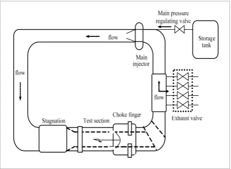
The simplified schematic structure of the 2.4m wind tunnel is shown in Fig. 1. The storage tank is the high pressure air source and supply power for wind tunnel testing. The main pressure regulating valve is used to ensure the constant of the gas entering the wind tunnel. Thus there exists a closed control loop for main injector pressure. The scale model to be tested is set in the test section. The aerodynamic parameters of scale models are measured at given stagnation pressures and Mach numbers. The angle attack of scale model will change according to the test requirements after the flow field approaches steady, which will lead to the stagnation pressure and Mach number deviates from the set point. At the same time, the high-precision flow field is expected to recover by adjusting the main exhaust valve and the choke finger.

The high-speed air flow in the test section is generated and controlled by the wind tunnel. Some of the gas is exhausted through the main exhaust valve, while the rest continues to circle in the tunnel. Fig. 2 illustrates the inputs and outputs in wind tunnel system. The stagnation pressure (y1) and the Mach number ( y2 ) in the test section are two major controlled variables of the flow field.

Fig. 1 The schematic structure of the 2.4m wind tunnel

1 y 2 y 1 v 2 v 2 u 1 u + − 1 r 2 r + −

Fig. 2 The structure of the wind tunnel control system

8 analyzing the input-output characheristcs based on the available signals, the block-oriented model consists of three parts: 1) the exhaust valve subsystemthatcan be described by a single-input single output (SISO) linear model and identified by the recursive least squares (RLS) algorithm; 2) the choke finger subsystyem that exhibits a nonlinear characteristics and can be approximated by a SISO pseudo-Hammerstein (pseudo-H) model. In order to cope with the hard nonlinearities, the adaptive weighted recursive least squares (AW-RLS) algorithm is applied based on the internal variable estimations. Moreover, by the use of an adaptive weighted factor, the convergence properties are also enhanced; 3) the flow field subsystem that can be described by a input two-output (TITO) linear model. Since the computational burden deteriorates greatly along with larger dimensions, the hierarchical recursive least squares (H-RLS) algorithm is used to address this problem. Based on the hierarchical concept, the flow field is simpilified into several sub-models with fewer parameters and smaller dimensions. Finally, numerical results are presented to validate the modeling scheme and show its merits over the previous ones.

The rest of the paper is organized as follows. Section 2 introduces the structure and operation principle of the wind tunnel. In Section 3, the block-oriented model and structure for the wind tunnel system is introduced. The parameter identification algorithms are formulated in Section 4. Simulation results illustrating the performance of the model and the algorithms are presented in Section 5. Finally, the conclusions are summarized in Section 6.

2. Wind tunnel system description

In this section, the wind tunnel system structure is firstly introduced. Then the analysis of the input-output characteristics of the exhaust valve loop, choke finger loop and flow field are presented, which lays a foundation for the nonlinear block-oriented model in Section 3.

The simplified schematic structure of the 2.4m wind tunnel is shown in Fig. 1. The storage tank is the high pressure air source and supply power for wind tunnel testing. The main pressure regulating valve is used to ensure the constant of the gas entering the wind tunnel. Thus there exists a closed control loop for main injector pressure. The scale model to be tested is set in the test section. The aerodynamic parameters of scale models are measured at given stagnation pressures and Mach numbers. The angle attack of scale model will change according to the test requirements after the flow field approaches steady, which will lead to the stagnation pressure and Mach number deviates from the set point. At the same time, the high-precision flow field is expected to recover by adjusting the main exhaust valve and the choke finger.

The high-speed air flow in the test section is generated and controlled by the wind tunnel. Some of the gas is exhausted through the main exhaust valve, while the rest continues to circle in the tunnel. Fig. 2 illustrates the inputs and outputs in wind tunnel system. The stagnation pressure (y1) and the Mach

number ( y2 ) in the test section are two major

controlled variables of the flow field.

Fig. 1 The schematic structure of the 2.4m wind tunnel

1 y 2 y 1 v 2 v 2 u 1 u + − 1 r 2 r + −

(4)

cal connections and hydraulic servo valves [27]. The actuator nonlinearity may often cause oscillations, delays and inaccuracy, and degrade the performance of control systems [6,18]. Many identification methods are proposed for systems with backlash nonlinearities [2,4,17].

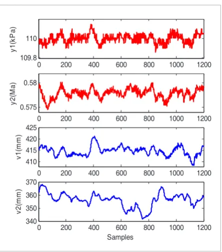
In the flow field, there exists high pressure and high speed air flow during the wind tunnel testing. For the compressibility and viscidity of air in closed circuit, changing any of the actuators influences the stagna-tion pressure and Mach number. Then input-output characteristics of the flow field are represented in Fig. 4. This part can be considered as a TITO linear model.

3. Modeling of the wind

tunnel system

In this section, the model of the wind tunnel is established based on the process actual data and structure characteristics. The online identificati-on aims to achieve the following goals: 1) to predict the dynamic behaviors of the process; and 2) to lay foundation for an on-line control strategy.

3.1 Block-oriented model of the wind tunnel By considering the backlash nonlinearity of the cho-ke finger loop, the nonlinear block-oriented model is introduced into the wind tunnel system. The exhaust valve subsystem (S1) is represented by a linear model. Figure 3

The structure of actuators

Figure 4

The input-output characteristics of the flow field

Figure 5

The block-oriented model diagram of wind tunnel

The choke finger subsystem (S2) is expressed as a pseudo-H model with input backlash. The coupled flow field subsystem (S3) is described as a TITO linear model. The block-oriented model diagram of the process is shown in Fig. 5.

For a wind tunnel, the signals u1 and u2 (the system in-puts), v₁ and v₂ (the position of the exhaust valve and the choke finger), y1 and y2 (the system outputs) are measurable; the variable x_{is the output of the backlash} (a) The control loops of exhaust valve

(b) The control loops of choke finger

9 2.2 The input-output characteristics of the exhaust valve loop, choke finger loop and flow field

The actuators of the wind tunnel are the main exhaust valve subsystem and choke fingersubsystem.Each of the subsystems is composed of a hydraulic servomechanism including a control loop. These two subsystems are mutually independent. The structures

ofthe exhaust valve loop and the choke finger loop are represented in Fig. 3. The actual

(

u1,u2

)

and outputs

(

v1,v2

)

of the actuators are available. By analyzingthe characteristics ofthe measured data, the

exhaust valve loop has a linear behavior, and the

choke finger loop has a nonlinear behavior.

The dynamiccharacteristics of theexhaust valve loop and the choke finger loop are neglected in the previous contributions [7,10,22]. However, the

prediction accuracy and control performance may deteriorate if the dynamic characteristics of actuators are not fully considered, especially the inherent nonlinear behavior of the choke finger loop. To this end, by analyzing the mechanical features and input

-output characteristics of the actuator, we try to introduce an input backlash into the modeling scheme. Later, the numerical results will verify the reasonableness of this novel idea. It is well known that backlash is particularly common in actuators, such as mechanical connections and hydraulic servo valves [27]. The actuator nonlinearity may often cause oscillations, delays and inaccuracy, and degrade the performance of control systems [6,18]. Many identification methods are proposed for systems with backlashnonlinearities [2,4,17].

In the flow field, there exists high pressure and high speed air flow during the wind tunnel testing. For the compressibility and viscidity of air in closed circuit, changing any of the actuators influencesthe stagnation pressure and Mach number. Then input

-output characteristics ofthe flow field are represented in Fig. 4. This part can be considered as a TITO linear model.

3. Modeling of the wind tunnel system

In this section, the model of the wind tunnel is

established based on the process actual data and structure characteristics. The online identification aims to achieve the following goals: 1) to predict the dynamic behaviors of the process; and 2) to lay foundation for an on-linecontrol strategy.

3.1 Block-oriented model of the wind tunnel

By considering the backlashnonlinearity of the choke

finger loop, the nonlinear block-oriented model is introduced into the wind tunnel system. The exhaust valve subsystem (S1) is represented by a linear model. The choke finger subsystem (S2) is expressed as a pseudo-H model with input backlash. The coupled flow field subsystem (S3) is described as a TITO

linear model. The block-oriented model diagram of the process is shown inFig. 5.

For a wind tunnel, the signals u1 and u2 (the system inputs), v₁ and v₂ (the position of the exhaust valve and the choke finger), y1 and y2 (the system outputs) are measurable; the variable x is the output of the backlash characteristic and is an unmeasurable intermediate signal; 1

1( ) G z− _, 1

2( )

G z− _and 1 3( ) G z− _are linear transfer functions with the unit time delay operator _z−1_.

1 v Exhaust valve 1 u Controller 1

a. The control loops of exhaust valve

Choke finger 2 v 2 u Controller 2

b. The control loops of choke finger Fig. 3The structure of actuators

0 200 400 600 800 1000 1200

109.8 110

y1(

kP

a)

0 200 400 600 800 1000 1200

0.575 0.58

y2(

M

a)

0 200 400 600 800 1000 1200

410 415 420 425 v1 (mm)

0 200 400 600 800 1000 1200

340 350 360 370 v2 (mm) Samples

Fig. 4The input-output characteristics of the flow field

2

u

1

u y1

2 y 2 v 1 v x Subsystem 1 1 1( ) G z−

1 2( ) G z− Subsystem 2

Subsystem 3

1 3( ) G z−

Fig. 5The block-oriented model diagram of wind tunnel

9 2.2 The input-output characteristics of the exhaust valve loop, choke finger loop and flow field

The actuators of the wind tunnel are the main exhaust valve subsystem and choke fingersubsystem.Each of the subsystems is composed of a hydraulic servomechanism including a control loop. These two subsystems are mutually independent. The structures

of the exhaust valve loop and the choke finger loop are represented in Fig. 3. The actual

(

u₁,u₂

)

and

outputs

(

v₁,v2

)

of the actuators are available. By analyzingthe characteristics ofthe measured data, the

exhaust valve loop has a linear behavior, and the

choke finger loop has a nonlinear behavior.

The dynamiccharacteristics of theexhaust valve loop and the choke finger loop are neglected in the previous contributions [7,10,22]. However, the

prediction accuracy and control performance may deteriorate if the dynamic characteristics of actuators are not fully considered, especially the inherent nonlinear behavior of the choke finger loop. To this end, by analyzing the mechanical features and input

-output characteristics of the actuator, we try to introduce an input backlash into the modeling scheme. Later, the numerical results will verify the reasonableness of this novel idea. It is well known that backlash is particularly common in actuators, such as mechanical connections and hydraulic servo valves [27]. The actuator nonlinearity may often cause oscillations, delays and inaccuracy, and degrade the performance of control systems [6,18]. Many identification methods are proposed for systems with backlashnonlinearities [2,4,17].

In the flow field, there exists high pressure and high speed air flow during the wind tunnel testing. For the compressibility and viscidity of air in closed circuit, changing any of the actuators influences the stagnation pressure and Mach number. Then input

-output characteristics ofthe flow field are represented in Fig. 4. This part can be considered as a TITO linear model.

3. Modeling of the wind tunnel system

In this section, the model of the wind tunnel is

established based on the process actual data and structure characteristics. The online identification aims to achieve the following goals: 1) to predict the dynamic behaviors of the process; and 2) to lay foundation for an on-linecontrol strategy.

3.1 Block-oriented model of the wind tunnel

By considering the backlashnonlinearity of the choke

finger loop, the nonlinear block-oriented model is introduced into the wind tunnel system. The exhaust valve subsystem (S1) is represented by a linear model. The choke finger subsystem (S2) is expressed as a pseudo-H model with input backlash. The coupled flow field subsystem (S3) is described as a TITO

linear model. The block-oriented model diagram of the process is shown inFig. 5.

For a wind tunnel, the signals u₁ and u₂ (the

system inputs), v1 and v2 (the position of the exhaust valve and the choke finger), y₁ and y₂ (the system outputs) are measurable; the variable x is the output of the backlash characteristic and is an unmeasurable intermediate signal; 1

1( ) G z− _, 1

2( )

G z− _and 1 3( ) G z− _are linear transfer functions with the unit time delay operator _z−1_.

1 v Exhaust valve 1 u Controller 1

a. The control loops of exhaust valve

Choke finger 2 v 2 u Controller 2

b. The control loops of choke finger Fig. 3The structure of actuators

0 200 400 600 800 1000 1200

109.8 110

y1(

kP

a)

0 200 400 600 800 1000 1200

0.575 0.58

y2(

M

a)

0 200 400 600 800 1000 1200

410 415 420 425 v1 (mm)

0 200 400 600 800 1000 1200

340 350 360 370 v2 (mm) Samples

Fig. 4The input-output characteristics of the flow field

2

u

1

u y1

2 y 2 v 1 v x Subsystem 1 1 1( ) G z−

1 2( ) G z− Subsystem 2

Subsystem 3

1 3( ) G z−

Fig. 5The block-oriented model diagram of wind tunnel

0 200 400 600 800 1000 1200

109.8 110

y1(

kP

a)

0 200 400 600 800 1000 1200

0.575 0.58

y2

(M

a)

0 200 400 600 800 1000 1200

410 415 420 425 v1 (mm)

0 200 400 600 800 1000 1200

340 350 360 370 v2 (mm) Samples 2 u 1

u y1

2 y 2 v 1 v x 1 1( ) G z

1 2( ) G z

1 3( ) G z

2( ) u t R m R

c

L m ( ) x t L c  Actuator Backlash 2( )

u t x t( )

(5)

407

Figure 6

An input-output map of backlash

characteristic and is an unmeasurable intermediate signal; 1

1( ) G z- _, 1

2( )

G z- _and 1 3( )

G z- _{are linear transfer}

functions with the unit time delay operator _z-1_.

3.2 Modeling of the exhaust valve subsystem S1 The following linear difference equation can describe the dynamics of the subsystem S1

1 1 1

1 1

( ) me _i ( ) ne _j ( )

i j

v t b u t i a v t j

= =

=

∑

⋅ - -

∑

⋅ - (1)

wherea a1, , ,2 ane, b b1, , ,2  bme

are the parameters to be estimated. The orders me, ne are known a prior.

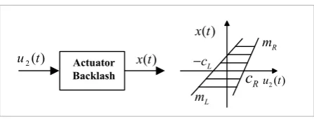
3.3 Modeling of the choke finger subsystem S2 A pseudo-H model with backlash is used to capture the dynamics of the subsystem S2. The input backlash of the pseudo-H model is shown in Fig. 6.

The mathematical models for the discrete-time case

are the u-axis values of the intersections, with the hori-zontal inner segment containing the slopes m_L and m_R. In order to simplify the backlash description and esti-mate the backlash parameters, the switching function h(.) is defined as

0 0

( )

1 0.

s h s

s > 

=  _≤

 (5)

To describe three branches of (2) in one equation, the following variables are defined for the description of backlash

[

]

[

]

{

}

1 2

2 2

( ) ( )

( ) ( 1) /

L

L L L L

f t h u t z

h m u t m c v t m

=

-= + - - (6)

[

]

[

]

{

}

2 2 2

2 2

( ) ( )

( 1) ( ) / .

R

R R R R

f t h z u t

h v t m u t m c m

=

-= - - + (7)

In order to obtain the input and output parameters equations of the backlash input block, we rewrite (2) as

[

][

]

2 1 1 2 2

2 1 2

( ) ( ) ( ) ( ) ( ) ( )

( ) ( 1) 1 ( ) 1 ( ) .

L L L R

R R

x t m u t f t m c f t m u t f t

m c f t x t f t f t

= + +

- + - - - (8)

It is clear that the linear part of the pseudo-H model can be written as follows:

1

2( ) 2( ) ( )

v t ₌G z x t

-(9)

where the linear transfer functions 1 2( ) G z- _are

defined as follows

1 2

1

2 1 2

1 2

... ( )

1 ...

mf mf

nf nf

b z b z b z

G z

a z a z a z

- -

-- -

-+ + +

=

+ + + + (10)

where a a1, , ,2  anf, b b1, , ,2  bmf_{are the unknown}

pa-rameters to be estimated; mf, nf are the orders of the linear block.

Substituting Eq. (8) into (9) yields the following in-put-output relationship

2 2 2

1 1

( ) mf _i ( ) nf _j ( ).

i j

v t b x t i a v t j

= =

=

∑

⋅ - -

∑

⋅ - (11)

2 u

1

u y1

2 y 2

v 1 v

x

1 1( )

G z

1 2( )

G z

1 3( )

G z

2( ) u t

R

m

R

c

L

m

( )

x t

L

c



Actuator Backlash

2( )

u t x t( )

of the backlash characteristics are described by [5]

[

]

[

]

2 2

2

2 2

( ) , ( )

( ) ( 1), ( )

( ) , ( )

L L L

L R

R R R

m u t c u t z

x t x t z u t z

m u t c u t z

 + <



=_ - ≤ ≤

 _- _>



(2)

where mL, mR, cL>0, cR >0are the unknown backlash parameters, and

( 1)

L L

L

x t

z c

m

-= - ₍₃₎

( 1)

R R

R

x t

z c

m

(6)

3.4 Modeling of the flow field subsystem S3 A multivariable coupled linear model is used to describe the dynamics of the subsystem S3. The inputs of the model are the positions of exhaust valve (v₁) and choke finger (v₂), and the outputs of the model are stagnation pressure (y1) and Mach number (y2). Then the flow field model 1

3( )

G z- _{is defined as}

1 1 1 1 2 2 2

1 1

1 1 2 2

1 1

( ) ( ) ( ) ( ) ( )

( ) ( ) ( ) ( )

a b

c d

n n

i j

n n

k l

y t b t v t d i b t v t d j

a t y t k a t y t l

= =

= - - + -

-+ - +

-∑

∑

(12)

2 1 1 1 2 2 2

1 1

1 1 2 2

1 1

( ) ( ) ( ) ( ) ( )

( ) ( ) ( ) ( )

a b

c d

n n

i j

n n

k l

y t b t v t d i b t v t d j

a t y t k a t y t l

= =

= - - + -

-+ - +

-∑

∑

(13)

where b t1i( ), b t2j( ), a t1k( ), a t2l( ), b t1i( ), b t2j( ), a t1k( ),

2l( )

a t are the unknown parameters. The orders n_a, n_b,

c

n, nd, na, nb, nc, nd and the time delays d1, d2, d1, d2 are assumed to be known.

4. Parameter estimation scheme

Parameter estimation is based on available data measured from the wind tunnel process. Three suitable recursive identification methods are applied to these subsystems.

4.1 Parameter estimation for exhaust valve subsystem

To estimate the parameters in (1), the recursive identification algorithm [11] has been used. Define the following parameter and data vectors:

1 [ , ,... , , ,... ]1 3 1 2 T

v b b b a ame ane

θ = (14)

1 1 1 1

1 1 1

( ) [ ( 1), ( 2),..., ( ),

( 1), ( 2),... ( )] .

v

T

t u t u t u t me

v t v t v t ne

φ = - -

-- - - (15)

The output equation (1) can be rewriten in a compact form

1( ) v1T( ) .v1

v t =ϕ tθ (16)

The estimates of parameter vector can be evaluated using the RLS algrithm. Firstly, define the output error

1( ) 1( ) T1( ) ( )ˆ1

v v v

e t =v t -φ tθ t (17)

based on (16), where θˆ ( )v1 t is the estimate of the parameter vector θ_v₁( )t .

Then the recursive identification algorithm is as follows:

1 1 1 1

ˆˆ ( )v t v ( 1)t K t e tv ( ) ( )v

θ =θ - + ₍₁₈₎

1 1

1

1 1 1 1

( 1) ( ) ( )

( ) ( 1) ( )

v v

v T

v v v v

P t t

K t

t P t t

φ

λ φ φ

-=

+ - (19)

1( ) 1( 1) 1( ) ( ) ( 1)T1 1

v v v v v

P t =P t- -K tφ t P t- (20)

where ₁ [ , ,... , , ,... ]ˆˆˆ₁ ₃ ˆˆˆ₁ ₂ T v b b b a ame ane

θ = . To initialize the

recursive algorithm in (17)-(20), we take Pv₁(0)=µv₁I ,

1 1

ˆ (0)v v [1,1, 1]

θ =ε ×  , where µ_v₁∈[10 ,10 ]4 10 , Iis the

unit matrix, ε λ ≤v1, v1 1 is the weighting term.

4.2 Parameter estimation for choke finger subsystem

The AW-RLS method [29] is used to estimate the pa-rameters of the pseudo-H model.

The output equation of (11) is a very complex expression. In order to obtain the separated variable

( 1)

x t- , according to the key term separation princi-ple [21], we can assume without loss of generality that

1 1

b = in (11). Then substituting (8) into (11) yields the following equation:

[

][

]

2 2 1 1

2 2 2

2 1 2

2 3

1 2 2 2 2

( ) ( 1) ( 1) ( 1)

( 1) ( 1) ( 1)

( 2) 1 ( 1) 1 ( 1)

( 2) ( 3) ( )

( 1) ( 2)... ( ).

L L L

R R R

mf

nf

v t m u t f t m c f t

m u t f t m c f t

x t f t f t

b x t b x t b x t mf

a v t a v t a v t nf

= - - +

-+ - - -

-+ - - - -

-+ - + - +

-- - -

-

(21)

Define the unknown parameter vector θv2

2

2 3 1 2

[ , , , ,

, ,... , , ,... ]

v L L L R R R

T

mf nf

m m c m m c

b b b a a a

θ =

(7)

409

and the information vector φ_v₂( )t

2 2 1 1

2 2 2

2

2 2

( ) [ ( 1) ( 1), ( 1),

( 1) ( 1), ( 1), ( 2),

( 3),..., ( ), ( 1),

( 2),..., ( )] .

v

T

t u t f t f t

u t f t f t x t

x t x t mf v t

v t v t nf

ϕ = - -

-- - - -

-- - -

-(23)

Then the parameterized pseudo-H model (21) can be rewritten as follows:

[

][

]

2( ) ( 2) 1 1( 1) 1 2( 1) v2T( ) .v2

v t -x t- -f t- -f t- =ϕ tθ

(24)

In order to estimate the parameters, we introduce the estimates θˆ_v₂ of the parameter vector θ_v₂

2 2 3 1 2 ˆ _{( ) [ ( ), ( ) ( ), ( ),}_ˆˆˆˆ ˆˆ ˆˆ ( ) ( ), ( ), ( ),..., ˆ _{( ), ( ), ( ),..., ( )] .}_ˆˆˆ

v L L L R

R R

T

mf nf

t m t m t c t m t m t c t b t b t b t a t a t a t

θ =

(25)

The predicted output at time t is

[

][

]

2 2 2

1 2

ˆ

ˆ ( ) ( ) ( 1)

( 2) 1 ( 1) 1 ( 1) .

T

v v

v t t t

x t f t f t

ϕ θ

=

-+ - - - (26)

The output error is

[

][

]

2 2 2 2

1 2

ˆ

( ) ( ) ( ) ( 1)

( 2) 1 ( 1) 1 ( 1) .

T

v v v

e t v t t t

x t f t f t

ϕ θ

= -

-- - - (27)

Providing that the internal auxiliary variables

{

f t f t x t1( ), ( ), ( )2

}

t=1,2,... are totally known, based on (23)-(27), we can update θˆ ( )v2 t according to the following weighted RLS algorithm

[

][

]

2 2 2 2

1 2

ˆ

( ) ( ) ( ) ( 1)

( 2) 1 ( 1) 1 ( 1) .

T

v v v

e t v t t t

x t f t f t

ϕ θ

= -

-- - - (28)

2 2

2 2 2 2

( ) ( 1)

( 1) ( ) ( ) ( 1)

( ) ( ) ( 1) ( )

v v

T

v v v v

T

v v v v

P t P t

P t t t P t

t t P t t

ϕ ϕ λ ϕ ϕ = -- -+ -(29) 2 2 3 1 2 ˆ _{( ) [ ( ), ( ) ( ), ( ),}_ˆˆˆˆ ˆˆ ˆˆ ( ) ( ), ( ), ( ),..., ˆ _{( ), ( ), ( ),..., ( )]}_ˆˆˆ

v L L L R

R R

T

mf nf

t m t m t c t m t m t c t b t b t b t a t a t a t

θ =

(30)

where λ_v₂( )t is the weighting term.

However, since the true innovation e t_v₂( ) and the in-formation vector ϕv₂( )t contain internal auxiliary

va-riables

{

f t f t x t₁( ), ( ), ( )₂

}

_t₌_1,2,..., which are generally un-measurable. Thus the parameter estimation cannot be performed directly on the basis of (28)-(30). Motivated by the ideas in [27], we replace the true counterparts e t_v₂( ) and ϕ_v₂( )t with the estimated innovation e tˆ ( )v₂ and the estimated information

vector ϕˆ ( )v2 t . The internal variable estimations

{

f t f t x tˆˆ1( ), ( ), ( )2 ˆ

}

_t₌_1,2,... are used to derive e tˆ ( )v2 and 2

ˆ ( )v t

ϕ . Then, the AW-RLS algorithm based on the internal variables estimations is as follows:

2 2

1 2 2

2 2 2 2

ˆˆ ( ) ( 1)

ˆ

( 1) ( ) ( ) ˆˆ

( ) ( ) ( 1) ( )

v v

T

v v v v

t t

P t t e t

t t P t t

θ θ ϕ λ ϕ ϕ = -+ + -(31) 2 2

2 2 2 2

( ) ( 1)

ˆˆ

( 1) ( ) ( ) ( 1) ˆˆ ( ) ( 1) ( )

v v

T

v v v v

T

v v v v

P t P t

P t t t P t

t P t t

ϕ ϕ λ ϕ ϕ = -- -+ -(32)

2 2 2 2

1 2

ˆ ˆ

ˆˆ ( ) ( ) ( ) ( 1)

ˆˆ

( 2) 1 ( 1) 1 ( 1)

T

v v v

e t v t t t

x t f t f t

ϕ θ

= -

-   

- - _ - - _{ } - - _ (33)

2 2 1 1

2 2 2

2

2 2

ˆˆ

ˆ ( ) [ ( 1) ( 1), ( 1),

ˆˆ _ˆ

( 1) ( 1), ( 1), ( 2),

ˆˆ( 3),... ( ), ( 1),

( 2),... ( )]

v

T

t u t f t f t

u t f t f t x t

x t x t mf v t

v t v t nf

ϕ = - - -- - - - -- - - -- - - -(34) 1 2 ˆ_{( )} _{{[ ( ) ( )}_ˆˆˆ _{( ) ( )}

ˆˆ( 1)] / ( )}L L L L

f t h m t u t m t c t

x t m t

= +

- - (35)

2 2

ˆ_{( )} _{{[ ( 1)}_ˆˆ _{( ) ( )}

ˆˆˆ ( ) ( )] /_R _R R_R( )}

f t h x t m t u t

m t c t m t

=

-+ (36)

2 1 1

2 2 2

1 2 ˆˆ ˆˆˆˆ( ) ( ) ( ) ( ) ( ) ( ) ( ) ˆˆ ˆˆˆ ( ) ( ) ( ) ( ) ( ) ( ) ˆˆ

ˆ( 1) 1 ( ) 1 ( ) .

L L L

R R R

x t m t u t f t m t c t f t m t u t f t m t c t f t

x t f t f t

= +

+

-   

+ - _ - _{ } - _

(37)

(8)

2( ) 1ˆˆT2( ) ( ) ( )2 2 2

v t v t P tv v t

λ =ε φ φ +ε (38)

where ε₁ and ε₂ are positive real numbers. At the beginning of the identification process, especially for bad initial conditions, a larger ε₁ is beneficial to convergence properties. On the other hand, the term

1 2ˆˆ ( ) ( ) ( )vT t P tv2 v2 t

ε φ φ tends to zero as the estimates approach the true values. Inevitably, a small ε2 is also required to guarantee a high convergence speed. To initialize the recursive algorithm in (31)-(34), we take P_v₂(0)=ρ_v₂₁I, where ρ_v₂₁ is a large positive sca-lar, e.g., 5

21 10

v

ρ = and θˆ (0)v2 =ρv22×[1,1, ,1] T, where 22

v

ρ is a small positive scalar, e.g., 2 22 10

v

ρ ₌ -_.

4.3 Parameter estimation for the flow field subsystem

The wind tunnel is a rapid sampling system and the sampling time is 10ms to 50ms. According to the principle of aerodynamics and the analysis of the actual data, the variation between adjacent ele-ments sampling interval is small. Therefore, the flow field subsystem can be considered as a TITO slowly time-varying linear process.

Since the computational burden deteriorates greatly along with larger dimensions, the H-RLS algorithm is used to address this problem. The basic idea of H-RLS is to decompose the identification model into several sub-models with fewer parameters and smaller di-mensions. It is proven that the H-RLS algorithm re-tains much less computational burden than the RLS algorithm [3, 28].

Then the flow field subsystem is identified by the following H-RLS algorithm.

Step1.Decomposition

Define the parameter vectors θw1( )t ,θw2( )t , and the information vectors ϕ_w₁( )t ,ϕ_w₁( )t for the wind tunnel flow field in (20) and (21)

1 11 1 21 2

11 1 21 2

( ) [ ( ), , ( ), ( ), , ( ),

( ), , ( ), ( ), , ( )]

a b

c d

w n n

T

n n

t a t a t a t a t

b t b t b t b t

θ =  

  (39)

2 11 1 21 2

11 1 21 2

( ) [ ( ), , ( ), ( ), , ( ),

( ), , ( ), ( ), , ( )]

a b

c d

w n n

T

n n

t a t a t a t a t

b t b t b t b t

θ =  

  (40)

1 1 1 2

2 1 1 1 1

2 2 2 2

( ) [ ( 1), , ( ), ( 1), ,

( ), ( ), , ( ),

( ), , ( )]

w a

b c

T d

t y t y t n y t

y t n v t d v t d n

v t d v t d n

ϕ = - -

-- -

- 



(41)

2 1 1 2

2 1 1 1 1

2 2 2 2

( ) [ ( 1), , ( ), ( 1), ,

( ), ( ), , ( ),

( ), , ( )] .

w a

b c

T d

t y t y t n y t

y t n v t d v t d n

v t d v t d n

ϕ = - -

-- -

- 



(42)

Equations (12) and (13) can be rewritten in a regres-sive form

1( ) wT1( ) ( )w1

y t =ϕ tθ t (43)

2( ) wT2( ) w2( ).

y t =ϕ tθ t (44)

The system in (43) and (44) is decomposed into two subsystems, respectively, and consequently the para-meter vectors θ_w₁( )t and θ_w₂( )t are decomposed into two sub-parameter vectors

1( ) [ T1 ( ), T1 ( )]T

w t w a t w b t

θ = θ θ (45)

2( ) [ T2 ( ), T2 ( )]T

w t w a t w b t

θ = θ θ (46)

and the information vectors ϕw1( )t and ϕw2( )t are de-composed into two sub-information vectors

1( ) [ T1 ( ), T1 ( )]T

w t w y t w v t

ϕ = ϕ ϕ (47)

2( ) [ T2 ( ); T2 ( )]T

w t w y t w v t

ϕ = ϕ ϕ (48)

where the vectors θ_{w a}₁ ( )t , θ_{w b}₁ ( )t , θ_{w a}₂ ( )t , θ_{w b}₂ ( )t , 1 ( )

w y t

ϕ , ϕw v₁ ( )t , ϕw y2 ( )t and ϕw v2 ( )t in (46)-(49) are defined as follows

1 ( ) [ ( ), ,11 1a( ), ( ), ,21 2b( )]

T w a t a t a t a tn an t

θ =   ₍₄₉₎

1 ( ) [ ( ), ,11 1c( ), ( ), ,21 2d( )]

T w b t b t b t b tn bn t

θ =   ₍₅₀₎

2 ( ) [ ( ), ,11 1a( ), ( ), ,21 2b( )]

θ =   ₍₅₁₎

2 ( ) [ ( ), ,11 1c( ), ( ), ,21 2d( )]

T w b t b t b t b tn bn t

θ =   ₍₅₂₎

1 1 1

2 2

( ) [ ( 1), , ( ),

( 1), , ( )]

w y a

T b

t y t y t n

y t y t n

ϕ = -

--

-

(9)

411

1 1 1 1 1

2 2 2 2

( ) [ ( ), , ( ),

( ), , ( )]

w v c

T d

t v t d v t d n

v t d v t d n

ϕ = -

-- -

-

 (54)

2 1 1

2 2

( ) [ ( 1), , ( ),

( 1), , ( )]

w y a

T b

t y t y t n

y t y t n

ϕ = -

--

-

 (55)

2 1 1 1 1

2 2 2 2

( ) [ ( ), , ( ),

( ), , ( )] .

w v c

T d

t v t d v t d n

v t d v t d n

ϕ = -

-- -

-

 (56)

According to the H-RLS principle [29], the equations (43) and (44) can be written in the following hierar-chical forms

1( ) w vT1 ( ) w b1 ( ) w yT1 ( ) w a1 ( )

y t -ϕ tθ t =ϕ tθ t (57)

1( ) w yT1 ( ) w a1 ( ) Tw v1 ( ) w b1 ( )

y t -ϕ tθ t =ϕ tθ t (58)

2( ) Tw y2 ( ) w a2 ( ) Tw v2 ( ) w b2 ( )

y t -ϕ tθ t =ϕ tθ t (59)

2( ) Tw y2 ( ) w a2 ( ) Tw v2 ( ) w b2 ( ).

y t -ϕ tθ t =ϕ tθ t (60)

Step2. Sub-models identification

According to the recursive least squares principle, we can derive the identification algorithm for each sub-system. Let θˆ ( )w a1 t , θˆ ( )w b1 t , θˆ ( )w a2 t and θˆ ( )w b2 t denote the estimates of the parameter vectors in (49)-(52).

1 11 1 21 2

ˆ _{( ) [ ( ), ,}_ˆˆˆˆ _{( ), ( ), ,} _{( )]}

a b

θ =   (61)

1 ˆˆˆˆ11 1 21 2

ˆ ( ) [ ( ), , ( ), ( ), , ( )]_c _d T

w b t b t b t b tn bn t

θ =   (62)

2 11 1 21 2

ˆ _{( ) [ ( ), ,}ˆˆˆˆ _{( ), ( ), ,} _{( )]}

a b

θ =   (63)

2 ˆˆˆˆ11 1 21 2

ˆ ( ) [ ( ), , ( ), ( ), , ( )] ._c _d T

w b t b t b t b tn bn t

θ =   (64)

For the hierarchical models (57) and (58), the parameter estimates can be updated as follows

1 1 1 1 1

1 1 1 1

ˆˆ ( ) ( 1) ( ) ( ) [ ( )

ˆ

( ) ( ) ( ) ( 1)]

w a w a w y

T T

w v w b w y w a

t t P t t y t

t t t t

θ θ ϕ

ϕ θ φ θ

= - + ×

- - - (65)

1 1 1 1

1 1

1 1 1

( 1) ( ) ( ) ( 1)

( ) ( 1)

1 ( ) ( 1) ( )

T

w y w y

T

w y w y

P t t t P t

P t P t

t P t t

ϕ ϕ

-

-=

-+ - (66)

1 1 2 1 1

1 1 1 1

ˆˆ ( ) ( 1) ( ) ( ) [ ( )

ˆ

( ) ( ) ( ) ( 1)]

w b w b w v

T T

w y w a w v w b

t t P t t y t

t t t t

θ θ ϕ

ϕ θ φ θ

= - + ×

- - - (67)

2 1 1 1

2 2

1 1 1

( 1) ( ) ( ) ( 1)

( ) ( 1)

1 ( ) ( 1) ( )

T

w v w v

T

w v w v

P t t t P t

P t P t

t P t t

ϕ ϕ

-

-=

-+ - (68)

where P t₁( ) and P t₂( ) are the covariance matrix of the sub-models. However, there is a difficulty that the equations (65) and (67) contain unknown parame-ter vectors. Then, by means of the coordination idea based on the hierarchical identification principle, we present a new algorithm to deal with the problem.

Step3.Coordination

The coordination idea is to replace the unknown vectors θw a1 ( )t and θw b1 ( )t which appear in (65) and (67) by their corresponding estimates θˆ ( 1)_{w a}₁ t- and

1

ˆ ( 1)_{w b} t

θ - at the preceding time, so we have

1 1 1 1 1

1 1 1 1

ˆˆ ( ) ( 1) ( ) ( ) [ ( )

ˆˆ

( ) ( 1) ( ) ( 1)]

w a w a w y

T T

w v w b w y w a

t t P t t y t

t t t t

θ θ ϕ

ϕ θ φ θ

= - + ×

- - - - (69)

1 1 1 1

1 1

1 1 1

( 1) ( ) ( ) ( 1)

( ) ( 1)

1 ( ) ( 1) ( )

T

w y w y

T

w y w y

P t t t P t

P t P t

t P t t

ϕ ϕ

-

-=

-+ - (70)

1 1 2 1 1

1 1 1 1

ˆˆ ( ) ( 1) ( ) ( ) [ ( )

ˆ

( ) ( 1) ( ) ( 1)]

w b w b w v

T T

w y w a w v w b

t t P t t y t

t t t t

θ θ ϕ

ϕ θ φ θ

= - + ×

- - - - (71)

2 1 1 1

2 2

1 1 1

( 1) ( ) ( ) ( 1)

( ) ( 1) .

1 ( ) ( 1) ( )

T

w v w v

T

w v w v

P t t t P t

P t P t

t P t t

ϕ ϕ

-

-=

-+ - (72)

Then, we can get the parameter estimates θˆ_{w a}₁ and θˆ_{w b}₁. To initialize the H-RLS algorithm, we take

1(0) 1

P =µI, θˆ (0)w a1 =ε1[1,1, ,1] T, P2(0)=µ2I and

1 2

ˆ (0) [1,1, ,1]T

w b

θ =ε  , where µ₁ and µ₂ are large

positi-ve scalars, e.g., 4 10

1, 2 [10 ,10 ]

µ µ ∈ . I is the unit matrix,

1

ε and ε₂ are small positive scalars.

In the same way, we can obtain the parameter estima-tes θˆw a2 and θˆw b2.

5. Model test and application

(10)

(RMSE) and Maximum absolute error (MAE). These performance criteria are defined as follows:

2

1

ˆ

( ( ) ( ))

N

t y t y t

RMSE

N

=

-=

∑

(73)

{

ˆ

}

max ( ) ( ) , 1

MAE= y t -y t t= N (74)

where y tˆ( ) denotes the predictive value,_{y t}_{( )} denotes

the actual value, N is the number of validation data. 5.1 Simulation and verification

The data of two operating conditions are used for parameter estimation and model verification. These two operating conditions are: 1) stagnation pressure 110kPa, Mach number 0.578, and 2) stagnation pres-sure 130kPa, Mach number 0.822. In this section, the sampling period is selected as 50ms.

The orders of the systems are determined by the false nearest neighbor algorithm [22]. Therefore, we choose

1

me ne= = , mf =1, nf =2，n_a =n_b =n_c =n_d =2 and

2

a b c d

n =n =n =n = . We select the time delay d₁, d₂, 1

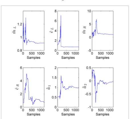
d and d₂ as 1. The parameter estimation results of the exhaust valve subsystem and the choke finger subsystem are shown in Figs. 7-8 and Table 1. The unit of the parameters cL,cR is mm (millimeter).

From the identification results, we can see that it is reasonable to introduce the backlash nonlinearity into the choke finger loop.

Figure 7

Estimations of exhaust valve

Figure 8

Estimations of the choke finger model

Table 1

The convergent parameter estimates of the exhaust valve and choke finger models

exhaust valve choke finger

1

ˆ

a _bˆ₁ _m_ˆ_L mˆ_R _Cˆ_L _Cˆ_R _aˆ₁ _aˆ₂

-0.62 0.39 0.9 0.9 0.8 0.85 1.0 -0.17

8

Fig. 7 Estimations of exhaust valve

Fig. 8 Estimations of the choke finger model

Fig. 10 Identification results of pressure model parameters

Fig. 11 Identification results of Mach number model parameters

Fig. 9 shows the comparision results between the actual outputs and the predicted outputs of the identified exhaust valve subsystem and the choke finger subsystem. The former plot is the true (－) and predicted (…) outputs for the exhaust valve

subsystem. The latter plot is the true (－) and predicted (…) outputs for the choke finger subsystem.

This illustrates that the fitting performance between the predicted outputs and the actual outputs are satisfactory.

The parameter estimation results of the flow field are shown in Figs. 10-11. Note that Fig. 10 depicts the stagnation pressure parameter estimates of equation (40), and Fig. 11 depicts the Mach number parameter estimates of equation (41).

(11)

413

Figure 9

Measured and predicted outputs of the identified exhaust valve subsystem and the choke finger subsystem

8

Fig. 7 Estimations of exhaust valve

Figure 10

Identification results of pressure model parameters

Figure 11

Identification results of Mach number model parameters

8 Fig. 7 Estimations of exhaust valve

8

Fig. 7 Estimations of exhaust valve

Fig. 8 Estimations of the choke finger model

Fig. 10 Identification results of pressure model parameters

Fig. 11 Identification results of Mach number model parameters

number are shown in Figs. 12-13. It can be seen that the estimated outputs fit the measured data well. The comparison results between the proposed block-oriented model, ENN model and the conventional

Figure 12

(12)

Figure 13

The predicted value, measured values and modelling errors of Mach number

Table 2

Performance criteria for identified block-oriented and conventional models

Working condition

(P0/Ma) Model

RMSE MAE

P0 Ma P0 Ma

110/0.578

Block_oriented model 0.0256 0.00033 0.0937 0.0012

Conventional model 0.0287 0.0004 0.1252 0.0026

ENN model 0.0023 0.0010 0.135 0.0031

130/0.822

Block_oriented model 0.0367 0.0005 0.1105 0.0041

Conventional model 0.0391 0.0009 0.1843 0.0059

ENN model 0.0045 0.0011 0.1904 0.006

model [14] are shown in Table 2. It is obvious that both RMSE and MAE of the proposed model are better than the conventional model.

5.2 Verification on the control platform of wind tunnel

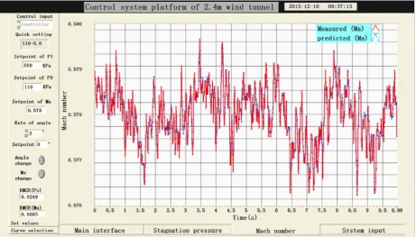
In order to verify the real-time performance of the proposed modeling scheme, further tests on the control platform of the wind tunnel system are carried out. The platform is equipped with several national instrument (NI) modules and created by La-bVIEW software. It can be used to test or optimize the

model and controller, and thus reduces the cost and risk during the controller design.

The experiments are performed in the following working condition: stagnation pressure 110kPa, Mach number 0.578. The control signals are given to both the obtained model and the actual wind tunnel. Then the measured outputs and the estimated outputs are displayed on the interface of the control platform, as shown in Figs. 14-15.

6. Conclusions

In this paper we present a nonlinear block-oriented model for the 2.4m wind tunnel. The block-oriented model consists of three parts: the main exhaust valve subsystem is represented as a linear model, the choke finger susystem is described as a pseudo-H model with input backlash, and the flow field subsystem is considered as a TITO linear model. In order to facil-itate the applications of the modeling scheme, the RLS, AW-RLS and H-RLS algorithms are presented for three subsystems. Finally, the results of simula-tions and control platform experiments show the va-lidity of the proposed modeling scheme.

Acknowledgments

(13)

415

Figure 14

The estimated stagnation pressure from block-oriented model and the measured data

Figure 15

(14)

References

1. Böling, J. M., Seborg, D. E., Hespanha, J. P. Multi-Model Adaptive Control of a Simulated pH Neutralization Pro-cess. Control Engineering Practice, 2007, 15(6), 663-672. https://doi.org/10.1016/j.conengprac.2006.11.008 2. Cerone, V., Regruto, D. Bounding the Parameters of

Li-near Systems with Input Backlash. IEEE Transactions on Automatic Control, 2007, 52(3), 531-536. http://dx. doi.org/10.1109/TAC.2007.892375

3. Ding, J., Ding, F., Liu, X. P., Liu,G. Hierarchical Least Squares Identification for Linear SISO Systems with Dual-Rate Sampled-Data. IEEE Transactions on Au-tomatic Control, 2011, 56(11), 2677-2683. http://dx.doi. org/10.1109/TAC.2011.2158137

4. Fang, L., Wang, J., Zhang, Q. Identification of Extended Hammerstein Systems with Hysteresis-Type Input Nonlinearities Described by Preisach Model. Nonli-near Dynamics, 2015, 79(2), 1257-1273. http://dx.doi. org/10.1007/s11071-014-1740-3

5. Giri, F., Bai, E. W. Block-Oriented Nonlinear System Identification. London, Springer, 2010.

6. Hägglund, T. Automatic On-line Estimation of Bac-klash in Control Loops. Journal of Process Control, 2007, 17(6), 489-499. https://doi.org/10.1016/j.jpro-cont.2007.01.002

7. Jin, Z. W., Zhao, L., Rao, Z. Z. Mach Number Predicti-on Models Based Predicti-on Ensemble Neural Networks for Wind Tunnel Testing. IEEE International Conferen-ce on Control and Decision, Chang Sha, China, 31 May – 2 June 2014, 1637-1640. http://dx.doi.org/10.1109/ CCDC.2014.6852430

8. Johansen, T. A., Foss, B. Constructing NARMAX Models Using ARMAX Models. International Jour-nal of Control, 1993, 58(5), 1125-1153. http:// dx.doi. org/10.1080/00207179308923046

9. Kaminskas, V., Liutkevičius, R. Adaptive Fuzzy Control of Pressure and Level. Information Technology and Control, 2009, 38(3), 233-236. http://itc.ktu.lt/index. php/ITC/article/view/12104/6752

10. Li, K., Peng, J. X., Rwin, G. W. A Fast Nonlinear Model Identification Method. IEEE Transactions on Auto-matic Control, 2005, 50(8), 1211-1216. http://dx.doi. org/10.1109/TAC.2005.852557

11. Ljung, L. System Identification: Theory for the User. Prentice Hall Information and System Sciences Series. Ed: Prentice Hall, New Jersey, 1999.

12. Liu, W., Pokharel, P. P., Principe, J. C. The Kernel Le-ast-Mean-Square Algorithm. IEEE Transactions on Signal Processing, 2008, 56(2), 543-554. http://dx.doi. org/10.1109/TSP.2007.907881

13. Liu, Y., Pan, Y., Sun, Z., Huang, D. Statistical Monito-ring of Wastewater Treatment Plants Using Variatio-nal Bayesian PCA. Industrial & Engineering Chemis-try Research, 2014, 53(8), 3272-3282. http://dx.doi. org/10.1021/ie403788v

14. Liu, Z. C. Measurement and Control System Design in High and Low Speed Wind Tunnel. National Defense Industry Press, Beijing, 2003.

15. Li, Y., Tong, S., Li, T. Observer-Based Adaptive Fuzzy Tracking Control of MIMO Stochastic Nonlinear Sys-tems with Unknown Control Directions and Unknown Dead Zones. IEEE Transactions on Fuzzy Systems, 2015, 23(4), 1228-1241. http://dx.doi.org/10.1109/TFU-ZZ.2014.2348017

16. Li, Y., Tong, S. Adaptive Fuzzy Output-Feedback Con-trol of Pure-Feedback Uncertain Nonlinear Systems with Unknown Dead Zone. IEEE Transactions on Fuzzy Systems, 2014, 22(5), 1341-1347. http://dx.doi. org/10.1109/TFUZZ.2013.2280146

17. Merzouki, R., Cadiou, J. C. Estimation of Backlash Phe-nomenon in the Electromechanical Actuator. Control Engineering Practice, 2005, 13(8), 973-983. https://doi. org/10.1016/j.conengprac.2004.10.016

18. Nordin, M., Gutman, P. O. Controlling Mechanical Systems with Backlash – A Survey. Automatica, 2002, 38(10), 1633-1649. https://doi.org/10.1016/S0005-1098(02)00047-X

19. Pupeikis, R. On Recursive Parametric Identification of Wiener Systems. Information Technology and Con-trol, 2011, 40(1), 21-28. http://dx.doi.org/10.5755/j01. itc.40.1.189

20. Pan, Y., Er, M. J., Li, X., Yu, H., Gouriveau, R. Machi-ne Health Condition Prediction Via OnliMachi-ne Dynamic Fuzzy Neural Networks. Engineering Applications of Artificial Intelligence, 2014, 35, 105-113. http://dx.doi. org/10.1016/j.engappai.2014.05.015

(15)

417

22. Rui, W., Qin, J., Ma, Y. A Novel Approach for Modelling of an Injector Powered Transonic Wind Tunnel. IEEE International Conference on Control and Decision, Chang Sha, China, 31 May – 2 June 2014, 1197-1200. http://dx.doi.org/10.1109/CCDC.2014.6852348

23. Seeger, M. Gaussian Processes for Machine Learning. International Journal of Neural Systems, 2004, 14(02), 69-106. https://doi.org/10.1142/S0129065704001899 24. Soeterboek, R. A., Pels, A. F., Verbruggen, H. B., van

Lan-gen, G. C. A Predictive Controller for the Mach Number in a Transonic Wind Tunnel. IEEE Control Systems, 1991, 11(1), 63-72. http://dx.doi.org/10.1109/37.103359 25. Vanbeylen, L. Nonlinear LFR Block-Oriented Model:

Potential Benefits and Improved, User-Friendly Iden-tification Method. IEEE Transactions on Instrumenta-tion and Measurement, 2013, 62(12), 3374-3383. http:// dx.doi.org/10.1109/TIM.2013.2272868

26. Verstraeten, D., Schrauwen, B., d’Haene, M., Strooban-dt, D. An Experimental Unification of Reservoir

Com-puting Methods. Neural Networks, 2007, 20(3), 391-403. https://doi.org/10.1016/j.neunet.2007.04.003 27. Vörös, J. Modeling and Identification of Systems with

Backlash. Automatica, 2010, 46(2), 369-374. https://doi. org/10.1016/j.automatica.2009.11.005

28. Wang, D. Q., Ding, F. Hierarchical Least Squares Esti-mation Algorithm for Hammerstein-Wiener Systems. IEEE Signal Processing Letters, 2012, 19(12), 825-828. http://dx.doi.org/10.1109/LSP.2012.2221704

29. Yu, F., Mao, Z., Jia, M. Recursive Identification for Hammerstein-Wiener Systems with Dead-Zone In-put Nonlinearity. Journal of Process Control, 2013, 23(8), 1108-1115. https://doi.org/10.1016/j.jpro-cont.2013.06.014

30. Yu, F., Mao, Z., Jia, M., Yuan, P. Recursive Parameter Identification of Hammerstein-Wiener Systems with Measurement Noise. Signal Processing, 2014, 105, 137-147. https://doi.org/10.1016/j.sigpro.2014.05.030

Summary / Santrauka

This paper develops a novel nonlinear block-oriented model for the wind tunnel system. Based on the avail-able signals, the wind tunnel system can be divided into three parts, namely, the exhaust valve loop, the choke finger loop and the flow field. Then the considered plant is described as a nonlinear block-oriented model. The exhaust valve subsystem and the flow field subsystem are both expressed by linear dynamic models, whereas the choke finger subsystem exhibits a nonlinear characteristics and is approximated by a pseudo-Hammer-stein model. Based on the above parameterization model, the recursive identification algorithms are presented for three subsystems. Interestingly, the adaptive weighted recursive least squares algorithm is applied to the pseudo-Hammerstein model, and the hierarchical recursive least squares algorithm is used to reduce the com-putational complexities. Both simulations and experiments are carried out to verify the effectiveness of the proposed method.