179 Information Technology and Control 2019/2/48
Optimized RRT-A* Path Planning
Method for Mobile Robots in
Partially Known Environment
ITC 2/48Journal of Information Technology and Control
Vol. 48 / No. 2 / 2019 pp. 179-194
DOI 10.5755/j01.itc.48.2.2139
Optimized RRT-A* Path Planning Method for Mobile Robots in Partially Known Environment
Received 2018/08/05 Accepted after revision 2019/04/06
http://dx.doi.org/10.5755/j01.itc.48.2.21390
Corresponding author: [email protected]
Ben Beklisi Kwame Ayawli
College of Electrical Engineering and Control Science, Nanjing Tech University, China.
Computer Science Department, Sunyani Technical University, Sunyani, Ghana, email: [email protected]
Xue Mei, Mouquan Shen
College of Electrical Engineering and Control Science, Nanjing Tech University, China
Albert Yaw Appiah, Frimpong Kyeremeh
College of Electrical Engineering and Control Science, Nanjing Tech University, China.
Electrical and Electronic Engineering Department, Sunyani Technical University, Sunyani, Ghana
This paper presents an optimized rapidly exploring random tree A* (ORRT-A*) method to improve the perfor-mance of RRT-A* method to compute safe and optimal path with low time complexity for mobile robots in par-tially known complex environments. ORRT-A* method combines morphological dilation, goal-biased RRT, A* and cubic spline algorithms. Goal-biased RRT is modified by introducing additional step-size to speed up the generation of the tree towards the goal after which A* is applied to obtain the shortest path. Morphological di-lation technique is used to provide safety for the robots while cubic spline interpodi-lation is used to smoothen the path for easy navigation. Results indicate that ORRT-A* method demonstrates improved path quality compared to goal-biased RRT and RRT-A* methods. ORRT-A* is, therefore, a promising method in achieving autonomous ground vehicle navigation in partially known environments.
KEYWORDS: Rapidly exploring random tree (RRT); mobile robots; path planning; morphological dilation; au-tonomous ground vehicles.
1. Introduction
In recent years, mobile robot path planning research has been an active research area gaining considerable attention [6, 26, 35]. Despite the immense research in
popular-Information Technology and Control 2019/2/48 180
ity in addressing mobile robot path planning problems [20]. Notable among these methods include probabi-listic roadmap (PRM) [33], voronoi diagram (VD) [4, 5] and rapidly exploring random tree (RRT) path plan-ning methods [1, 7, 9, 13, 14, 24, 25, 34, 37, 39]. Consid-eration is given to RRT path planning in this paper. RRT is a single query incremental algorithm [22] that generates a tree in a free configuration space until the defined target is reached[7, 18]. RRT is described as a fast path planning method that performs well in com-plex and high dimensional workspace[14, 39]. RRT is a good method for motion planning for mobile robots because of its strength in controlling inputs compu-tation [13]. It seeks to find a path between an initial state and target in a free configuration space with-out the representation of the entire environment. Recently, mobile robot path planning research using RRT and its variants has been widely considered. RRT trajectory planning method for car-like robots was proposed in [13], where uniform and goal-biased sampling technique was employed to generate the tree. Consideration was given to controlling input se-lection for the trajectory planning in urban, office and landscape environments. Generally, the major chal-lenge of the RRT method is the inability to control path quality [19, 21, 37]. However, no consideration was given by the authors to address the path quality problem. Although RRT is probabilistic complete, generated path is described to be far from optimal, because it tries to ensure computational efficiency at the expense of optimality [7, 37].
Intense study to improve the performance of RRT path planning method has been carried out over the years. RRT* algorithm, an extension of RRT was pro-posed in [19] which tried to improve path quality by computing asymptotically sub-optimal path. The tree structure of RRT* is flexible making it easy to improve path quality. Even though the RRT* ensures asymp-totic optimality [20] and performs better than RRT in terms of path optimality, it has high time complexity due to the continuous execution of the local planner during the generation of the tree [7]. It is reported to be difficult to perform dynamic path replanning us-ing RRT* [39]. Islam et al. [16] took advantage of the asymptotic optimality provision by RRT* to present RRT*-smart approach to increase the convergence rate of RRT method to improve path quality with low time complexity. To address slow convergence
181 Information Technology and Control 2019/2/48
which performs continuous path update during the navigation of the robot. Despite research progress to minimize the probability of RRT path generation and to enhance path construction, difficulty of controlling path quality still exists [28, 37].
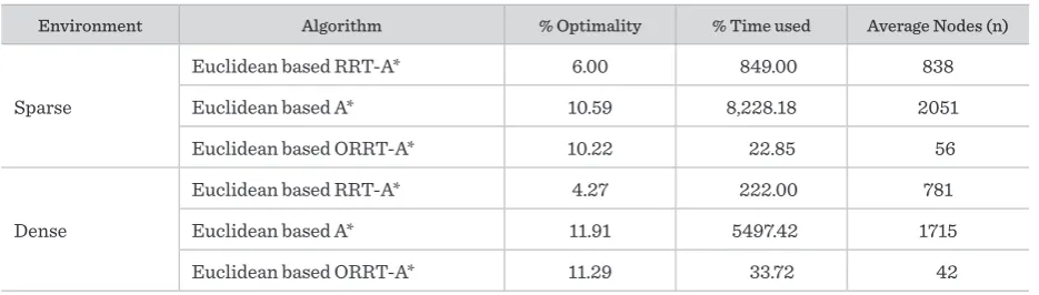
In recent years, RRT method has been combined with other path planning methods to help improve path quality. In [38], Gaussian process occupancy map was combined with RRT to plan secure path in cluttered environment. Tusi and Chung [34] combined RRT and artificial bee colony (ABC) methods. RRT algo-rithm was used in this method to generate nodes in the free configuration space and the best nodes were considered by applying ABC method to move the bees. The method was described to have performed bet-ter compared to particle swarm optimization (PSO) method. Any-angle search algorithm was combined with RRT to present theta*-RRT motion planning method for non-holonomic wheeled robots [29]. Theta*-RRT method was described to have generated shorter paths in shorter time compared to other RRT methods. To obtain near-optimal path of nonlinear dynamic mobile robots, Li et al. [23] combined neu-ral network and RRT to present NoD-RRT method. The authors considered the nonlinear kinodynamic constraints of the vehicles and revised RRT to per-form reconstruction to deal with the kinodynamic constraints problem. Results showed that NoD-RRT performed better compared to RRT and RRT*. An-other recent hybrid method involving RRT is RRT-A* motion planning method presented in [24]. The method focused on optimizing RRT path generation for non-holonomic mobile robots in known environ-ment. A* heuristic algorithm was used to decide the selection of the nearest node during the generation of the tree. The authors acknowledged the fact that the method suffered local minima problem. The authors indicated that the path length obtained using RRT-A* method was more optimal compared to goal-biased RRT method. This analysis, however, compared Man-hattan based RRT-A* to Euclidean based goal-bi-ased RRT which are of different metric functions as demonstrated in the paper. Comparing Euclide-an-based RRT-A* to EuclideEuclide-an-based goal-biased RRT from their results, the proposed method utilized 849% of the time to achieve 6% path length improve-ment in sparse environimprove-ment. In dense environimprove-ment, 222% time was used to achieve 4.27% path length improvement over Euclidean-based goal biased RRT.
But the rate of time used compared to achieved results indicates the method lacks some efficiency. The path quality problem of RRT and challenges identified in [24] motivated this research to optimize and extend RRT-A* method to produce better results.
Therefore, this paper presents an optimized RRT-A* path planning method based on morphological dila-tion (MD), goal-biased RRT, A* heuristic algorithm and cubic spline interpolation to compute safe and optimal path for autonomous mobile robots in par-tially known complex environment. A step size is usually used in goal-biased RRT for the generation of the RRT. In this paper, additional step-size is intro-duced to speed up the generation of the tree towards the goal based on the random sample value. In [24], A* heuristic function was applied at every iteration to select the nearest node during the generation of the tree which had high time cost in path computation. In this paper, the A* heuristic algorithm is used to optimize and obtain the shortest path after the path is generated using the modified goal-biased RRT. To provide safe and smooth path for feasible navigation, MD technique is used to inflate the obstacles before generating the path, and cubic spline interpolation (CSI) is used to smoothen the path. Path replanning is provided by generating new path from a current po-sition of the robot when a random obstacle obstructs its navigation path. ORRT-A* approach addresses the local minima problem reported with RRT-A* [24] and generates safe and optimal path with low time cost in partially known environment.
The rest of this paper is organized as follows. Problem formulation is given in Section 2. Section 3 describes the proposed methods: obtaining and processing map, computing the roadmap, path query and optimization, path smoothening, and replanning. The simulation re-sults and discussion are presented in Sections 4 and 5, respectively. Finally, Section 6 concludes the paper.
2. Problem Formulation
The configuration space CS of the mobile robot is represented in Figure 1. The CS is made up of re-gions with obstacles, CSobs and free configuration space CSfree. In this paper, environment of 2D where
2
Information Technology and Control 2019/2/48 182
Figure 1
The configuration space of a robot with sample obstacles and RRT path from the initial position v0 to the target vt applied at every iteration to select the nearest
node during the generation of the tree which had high time cost in path computation. In this paper, the A* heuristic algorithm is used to optimize and obtain the shortest path after the path is generated using the modified goal-biased RRT. To provide safe and smooth path for feasible navigation, MD technique is used to inflate the obstacles before generating the path, and cubic spline interpolation (CSI) is used to smoothen the path. Path replanning is provided by generating new path from a current position of the robot when a random obstacle obstructs its navigation path. ORRT-A* approach addresses the local minima problem reported with RRT-A* [24] and generates safe and optimal path with low time cost in partially known environment.
The rest of this paper is organized as follows. Problem formulation is given in Section 2. Section 3 describes the proposed methods: obtaining and processing map, computing the roadmap, path query and optimization, path smoothening, and replanning. The simulation results and discussion are presented in Sections 4 and 5, respectively. Finally, Section 6 concludes the paper.
2. Problem Formulation
The configuration space CS of the mobile robot is
represented in Figure 1. The CS is made up of
regions with obstacles, CSobs and free
configuration space CSfree. In this paper,
environment of 2D where CSR2 is considered.
Hence, CSobsCS and each vertex of CSobscan
be represented as vobs i( )Cobs. The CSfree can be obtained using CSfreeCS CS\ obs and each vertex of CSfree is given as vfree i( )CSfree. The RRT is
generated in the CSfree such that collision with
obs
CS is avoided. The generation of the tree starts
at the initial position of the vehicle and expands towards the target. Given the vertices of the tree from the initial state to the target as
0 1 2 3 ( , , , ,..., )
i t
V v v v v v , Vi represents positions in the CSfree. v0 is the initial position of the tree
while vt represents the target or the iteration
limit of the tree generation.
Figure 1
The configuration space of a robot with sample obstacles and RRT path from the initial position v0 to
the target vt
CSfree
CSobs1
v
0v
tCSobs2
CSobs6 CSobs3
CSobs4
v
1v
2v
3v
4v
5v
6This paper focuses on computing safe, shortest and smooth path in CSfree from v0 to vt using less time in partially known environment. At the initial state, the environment of the vehicle is assumed known during path computation. As the vehicle navigates to its target based on the computed path, random obstacles can obstruct the path leading to collision. This paper provides a reactive path replanning to avoid obstacles that obstruct the path of the vehicle during navigation in real-time.
3. Proposed Method
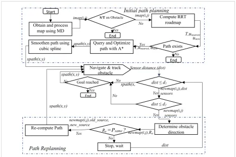
The general algorithms of the method presented in this paper are demonstrated in a workflow diagram in Figure 2. The path planning method presented in this paper has been divided into five steps: obtaining and processing map, computing the RRT roadmap, path query and optimization, path smoothening and path replanning.
Figure 2
Workflow diagram of the proposed method
and each vertex of CSfree is given as vfree i( )∈CSfree.
The RRT is generated in the CSfree such that colli-sion with CSobsis avoided. The generation of the tree starts at the initial position of the vehicle and expands
Figure 2
Workflow diagram of the proposed method
3.1 Step 1: Obtaining and Processing Map The map of the workspace could be obtained using camera or scanning laser range finder. The captured map of the environment is processed to give binary representations of the CSobs and the
free
CS of the CS. To ensure safety of the mobile robots during navigation such that the generated path is not too close to obstacles in the workspace to cause collisions, obstacles in the map are inflated before constructing the RRT roadmap using MD technique given in [12]. The dimension of the vehicle and other safety requirements are considered in inflating the obstacles. The MD equation denoted by P Q is given as:
{ | ( )i r }
P Q r Q P , (1)
where P represents the map, Q represents the
structure element for the dilation, r is the set of all nodes of the map and Qi denotes the reflection of the set Q. The MD of a given binary map with the matrix, bmap x y( , ) and a structuring element
q( , )x y can therefore, be calculated using Equation (2):
( ) max{ ( ) ( ) | (R ), & },
bmap q
bmap q R bmap R x q x x
S S
(2)
where S and R denote the dimension of the map and the translated radius representing the robot’s safety space required, respectively. Equation (2) is used to inflate the obstacles on the map before generating the tree to ensure safe navigation.
3.2 Step 2: Computing the RRT Roadmap Details of basic RRT algorithm are given in [1, 7, Path Replanning
spath(x,y)
newmap(i,j),dist sensors Yes
Navigate & track obstacle Goal reached
End
Re-compute Path Obtain and process
map using MD
S/T on Obstacle Compute RRT
roadmap
Path exists Query and Optimize
path with A* Smoothen path using
cubic spline
End
End Start
dist ≤ d1
Ra =Psame ? Determine obstacle direction
dist ≤ d2
Stop, wait
imap(i,j) imap(i,j)
T,unearest unew
No
Sensor distance (dist)
No
apath(x,y)
spath(x,y)
spath(x, Yes
No
T,unearest, unew
dist Yes
Yes
Yes
No
No
newmap(i,j) sensors
newmap(i,j),Ra
newmap(i,j),old_source, ,new_source
Initial path planning
No
spath(x,y)
Yes
towards the target. Given the vertices of the tree from the initial state to the target as Vi=( , , , ,..., )v v v v0 1 2 3 vt ,
i
V represents positions in the CSfree. v0 is the initial position of the tree while vt represents the target or the iteration limit of the tree generation.
This paper focuses on computing safe, shortest and smooth path in CSfree from v0 to
v
t using less time in partially known environment. At the initial state, the en-vironment of the vehicle is assumed known during path computation. As the vehicle navigates to its target based on the computed path, random obstacles can obstruct the path leading to collision. This paper provides a reac-tive path replanning to avoid obstacles that obstruct the path of the vehicle during navigation in real-time.3. Proposed Method
183 Information Technology and Control 2019/2/48
paper has been divided into five steps: obtaining and processing map, computing the RRT roadmap, path query and optimization, path smoothening and path replanning.
3.1. Step 1: Obtaining and Processing Map The map of the workspace could be obtained using camera or scanning laser range finder. The captured map of the environment is processed to give binary representations of the CSobs and the CSfree of the
CS. To ensure safety of the mobile robots during nav-igation such that the generated path is not too close to obstacles in the workspace to cause collisions, ob-stacles in the map are inflated before constructing the RRT roadmap using MD technique given in [12]. The dimension of the vehicle and other safety require-ments are considered in inflating the obstacles. The MD equation denoted by P Q⊕ is given as:
Figure 2
Workflow diagram of the proposed method
3.1 Step 1: Obtaining and Processing Map
The map of the workspace could be obtained using camera or scanning laser range finder. The captured map of the environment is processed to give binary representations of the CSobs and the
free
CS of the CS. To ensure safety of the mobile robots during navigation such that the generated path is not too close to obstacles in the workspace to cause collisions, obstacles in the map are inflated before constructing the RRT roadmap using MD technique given in [12]. The dimension of the vehicle and other safety requirements are considered in inflating the obstacles. The MD equation denoted by P Q⊕ is given as:
{ | ( )i r }
P Q⊕ = r Q ∩ ≠ ∅P , (1)
where P represents the map, Q represents the
structure element for the dilation, r is the set of all nodes of the map and Qi denotes the reflection of the set Q. The MD of a given binary map with the matrix, bmap x y( , ) and a structuring element
q( , )x y can therefore, be calculated using Equation (2):
( ) max{ ( ) ( ) | (R ),
& },
bmap q
bmap q R bmap R x q x x
S S
⊕ = − + −
∈ ∈ (2)
where S and R denote the dimension of the map and the translated radius representing the robot’s safety space required, respectively. Equation (2) is used to inflate the obstacles on the map before generating the tree to ensure safe navigation.
3.2 Step 2: Computing the RRT Roadmap
Details of basic RRT algorithm are given in [1, 7,
Path Replanning
spath(x,y) newmap(i,j),dist sensors YesNavigate & track obstacle Goal reached
End
Re-compute Path Obtain and process
map using MD
S/T on Obstacle Compute RRT
roadmap
Path exists Query and Optimize
path with A* Smoothen path using
cubic spline
End
End Start
dist ≤ d1
Ra
=Psame ?
Determine obstacle directiondist ≤ d2
Stop, wait
imap(i,j) imap(i,j)
T,unearest unew
No
Sensor distance (dist)
No apath(x,y) spath(x,y) spath(x, Yes No
T,unearest, unew
dist Yes Yes Yes No No newmap(i,j) sensors
newmap(i,j),Ra newmap(i,j),old_source,
,new_source
Initial path planning
No
spath(x,y)
Yes
(1)
where P represents the map, Q represents the struc-ture element for the dilation, r is the set of all nodes of the map and Qi denotes the reflection of the set Q. The MD of a given binary map with the matrix, bmap x y( , ) and a structuring element q( , )x y can therefore, be calculated using Equation (2):
( ) max{ ( ) ( ) | (R ),
& },
bmap q
bmap q R bmap R x q x x
S S
⊕ = − + −
∈ ∈ (2)
where S and R denote the dimension of the map and the translated radius representing the robot’s safety space required, respectively. Equation (2) is used to inflate the obstacles on the map before generating the tree to ensure safe navigation.
3.2. Step 2: Computing the RRT Roadmap Details of basic RRT algorithm are given in [1, 7, 13, 24, 25, 34, 37, 39]. This paper modifies and uses goal-biased RRT to generate the roadmap ensuring that the tree is rapidly generated towards the goal. The generation of the tree is biased towards the target when the random value rand to determine the compu-tation of the sample is less than the random threshold
rt. Two different step sizes, sz1 and sz2 are used with
sz2 assigned higher value than sz1. sz2 is used for the growth of the tree when the growth is biased to the target. This is aimed at reducing the number of nodes to be generated before reaching the target, thereby
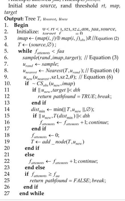
reducing the time and space complexity of the algo-rithm. The algorithm used in this paper to generate the roadmap is given in Algorithm 1.
Input: Step sizes sz1, sz2,Distance threshold dth Attempts allowed faa, Attempts fattempts,
Initial state source, rand threshold rt, map, target
Output: Tree T, unearest, unew
1. Begin
2. Initialize: 0 1, 1, 2,0 , , ,
tt t
rt sz sz dth faa source target f< < =
3 imap←(map i j( , )⊕map i j( , ) )obs R//Equation (2)
4. T←(source, )∅ ; 5. while fattempts< faa
6. sample rand imap target( , , ); // Equation (3) 7. urand ←sample;
8. unearest ←Nearest T u( , rand);// Equation (4)
9. unew(unearest,sz1,sz 2, );θ // Equation (6)
10. if ~CSobs(unew,imap)
11 if unew,target<dth
12 return pathfound TRUE break= ; ;
13 end if
14 distmin ←min( ,T unew, );∅
15 if unew, (T distmin)<dth 16 fattempts← fattempts+1;continue;
17 end if
18 fattempts ←0;
19 T←add node T u_ ( , new)
20 end if
21 else
22 fattempts← fattempts+1;continue;
23 end else
24 if fattempts≥ faa
25 return pathfound FALSE break= ; ;
26 end if
27 end while
28 End
The initial position of the robot represents the root of the tree, T ←(source, )∅ . The sample for generating the tree is computed as:
13, 24, 25, 34, 37, 39]. This paper modifies and uses goal-biased RRT to generate the roadmap ensuring that the tree is rapidly generated towards the goal. The generation of the tree is biased towards the target when the random value rand to determine the computation of the sample is less than the random threshold rt. Two different step sizes, sz1 and sz2 are used with sz2 assigned higher value than sz1. sz2 is used for the growth of the tree when the growth is biased to the target. This is aimed at reducing the number of nodes to be generated before reaching the target, thereby reducing the time and space complexity of the algorithm. The algorithm used in this paper to generate the roadmap is given in Algorithm 1.
The initial position of the robot represents the root of the tree, T←(source, )∅ . The sample for generating the tree is computed as:
{
randsample rand imap target(0,1)*(size imap(, ), if rand rt) .target otherwise
=
< (3)
The random value rand generated is compared to the random threshold rt. If rand < rt, a random sample is computed as given in Equation (3). The target is taken as the sample when rand ≥ rt to bias the growth of the tree towards the target. The nearest node, Nearest T u( , rand) is computed using
k-nearest neighbor (KNN) given as:
2 ( ) ( ) 1
( , rand) min k ( i rand i ) ,
i
Nearest T u T u
= = −
∑
(4)where urand =sample as given in Equation (3). The
direction
θ
to extend the sample to create new node is computed using Equation (5):2( rand nearest),
atan u u
θ= − (5) where unearest =Nearest T( ,urand) as given in Equation (4). The position of the new node unew is calculated using Equation (6):
{
( , 1, 2, )2*[sin cos ], , 1*[sin cos ],new nearest
nearest rand
nearest
u u sz sz
u sz if u target
u sz otherwise
θ
θ θ
θ θ
=
+ =
+ (6)
where sz1 and sz2 denote the step size 1 and 2, respectively. If urand =target, sz2 is used to
Algorithm 1
Computing the roadmap
Input: Step sizes sz1, sz2,Distance threshold dth Attempts allowed faa, Attempts fattempts,
Initial state source, rand threshold rt, map, target
Output: Tree T, unearest, unew
1. Begin
2. Initialize: 0 1, 1, 2,0 , , ,
tt t
rt sz sz dth faa source target f< < =
3 imap←(map i j( , )⊕map i j( , ) )obs R//Equation (2)
4. T←(source, )∅ ; 5. while fattempts< faa
6. sample rand imap target( , , ); // Equation (3) 7. urand ←sample;
8. unearest ←Nearest T u( , rand);// Equation (4) 9. unew(unearest,sz1,sz 2, );θ // Equation (6) 10. if ~CSobs(unew,imap)
11 if unew,target<dth
12 return pathfound TRUE break= ; ;
13 end if
14 distmin ←min( ,T unew, );∅
15 if unew, (T distmin)<dth
16 fattempts← fattempts+1;continue;
17 end if
18 fattempts ←0;
19 T←add node T u_ ( , new)
20 end if
21 else
22 fattempts← fattempts+1;continue;
23 end else
24 if fattempts≥ faa
25 return pathfound FALSE break= ; ;
26 end if
27 end while
28 End
compute the position of the new node unew towards the target with a higher step size. This is to facilitate the growth of the tree towards the target at a faster rate with reduced number of nodes. Collision checks are performed to ensure that the tree is generated within the CSfree. The growth of the tree ends once the target point is reached, or the iteration attempts fattempts exceed
the failed attempts allowed faa.
(3)
The random value rand generated is compared to the random threshold rt. If rand < rt, a random sample is computed as given in Equation (3). The target is tak-en as the sample whtak-en rand ≥ rt to bias the growth Algorithm 1
Information Technology and Control 2019/2/48 184
of the tree towards the target. The nearest node, ( , rand)
Nearest T u is computed using k-nearest
neigh-bor (KNN) given as:
13, 24, 25, 34, 37, 39]. This paper modifies and uses goal-biased RRT to generate the roadmap ensuring that the tree is rapidly generated towards the goal. The generation of the tree is biased towards the target when the random value rand to determine the computation of the sample is less than the random threshold rt. Two different step sizes, sz1 and sz2 are used with sz2 assigned higher value than sz1. sz2 is used for the growth of the tree when the growth is biased to the target. This is aimed at reducing the number of nodes to be generated before reaching the target, thereby reducing the time and space complexity of the algorithm. The algorithm used in this paper to generate the roadmap is given in Algorithm 1.
The initial position of the robot represents the root of the tree, T ←(source, )∅ . The sample for generating the tree is computed as:
{
randsample rand imap target(0,1)*(size imap(, ), if rand rt) .target otherwise
=
< (3)
The random value rand generated is compared to the random threshold rt. If rand < rt, a random sample is computed as given in Equation (3). The target is taken as the sample when rand ≥ rt to bias the growth of the tree towards the target. The nearest node, Nearest T u( , rand) is computed using k-nearest neighbor (KNN) given as:
2 ( ) ( ) 1
( , rand) min k ( i rand i ) ,
i
Nearest T u T u
= = −
∑
(4)where urand =sample as given in Equation (3). The direction
θ
to extend the sample to create new node is computed using Equation (5):2( rand nearest),
atan u u
θ = − (5) where unearest =Nearest T( ,urand) as given in
Equation (4). The position of the new node unew is calculated using Equation (6):
{
( , 1, 2, )2*[sin cos ], ,1*[sin cos ],
new nearest
nearest rand
nearest
u u sz sz
u sz if u target
u sz otherwise
θ
θ θ
θ θ
=
+ =
+ (6)
where sz1 and sz2 denote the step size 1 and 2, respectively. If urand =target, sz2 is used to
Algorithm 1
Computing the roadmap
Input: Step sizes sz1, sz2,Distance threshold dth Attempts allowed faa, Attempts fattempts,
Initial state source, rand threshold rt, map, target
Output: Tree T, unearest, unew
1. Begin
2. Initialize: 0 1, 1, 2,0 , , ,
tt t
rt sz sz dth faa source
target f< < =
3 imap←(map i j( , )⊕map i j( , ) )obs R//Equation (2) 4. T ←(source, )∅ ;
5. while fattempts < faa
6. sample rand imap target( , , ); // Equation (3) 7. urand ←sample;
8. unearest ←Nearest T u( , rand);// Equation (4)
9. unew(unearest,sz1,sz 2, );θ // Equation (6)
10. if ~CSobs(unew,imap)
11 if unew,target<dth
12 return pathfound TRUE break= ; ;
13 end if
14 distmin ←min( ,T unew, );∅ 15 if unew, (T distmin)<dth
16 fattempts ← fattempts +1;continue;
17 end if
18 fattempts←0;
19 T ←add node T u_ ( , new)
20 end if
21 else
22 fattempts ← fattempts+1;continue;
23 end else
24 if fattempts ≥ faa
25 return pathfound FALSE break= ; ;
26 end if
27 end while
28 End
compute the position of the new node unew towards the target with a higher step size. This is to facilitate the growth of the tree towards the target at a faster rate with reduced number of nodes. Collision checks are performed to ensure that the tree is generated within the CSfree. The growth of the tree ends once the target point is reached, or the iteration attempts fattempts exceed the failed attempts allowed faa.
(4)
where urand =sample as given in Equation (3). The di-rection
θ
to extend the sample to create new node is computed using Equation (5):13, 24, 25, 34, 37, 39]. This paper modifies and uses goal-biased RRT to generate the roadmap ensuring that the tree is rapidly generated towards the goal. The generation of the tree is biased towards the target when the random value rand to determine the computation of the sample is less than the random threshold rt. Two different step sizes, sz1 and sz2 are used with sz2 assigned higher value than sz1. sz2 is used for the growth of the tree when the growth is biased to the target. This is aimed at reducing the number of nodes to be generated before reaching the target, thereby reducing the time and space complexity of the algorithm. The algorithm used in this paper to generate the roadmap is given in Algorithm 1.
The initial position of the robot represents the root of the tree, T ←(source, )∅ . The sample for generating the tree is computed as:
{
randsample rand imap target(0,1)*(size imap(, ), if rand rt) .target otherwise
=
< (3)
The random value rand generated is compared to the random threshold rt. If rand < rt, a random sample is computed as given in Equation (3). The target is taken as the sample when rand ≥ rt to bias the growth of the tree towards the target. The nearest node, Nearest T u( , rand) is computed using k-nearest neighbor (KNN) given as:
2 ( ) ( ) 1
( , rand) min k ( i rand i ) ,
i
Nearest T u T u
= = −
∑
(4)where urand =sample as given in Equation (3). The direction
θ
to extend the sample to create new node is computed using Equation (5):2( rand nearest),
atan u u
θ = − (5) where unearest =Nearest T( ,urand) as given in Equation (4). The position of the new node unew is calculated using Equation (6):
{
( , 1, 2, )2*[sin cos ], ,1*[sin cos ],
new nearest
nearest rand
nearest
u u sz sz
u sz if u target
u sz otherwise
θ
θ θ
θ θ
=
+ =
+ (6)
where sz1 and sz2 denote the step size 1 and 2, respectively. If urand =target, sz2 is used to
Algorithm 1
Computing the roadmap
Input: Step sizes sz1, sz2,Distance threshold dth Attempts allowed faa, Attempts fattempts,
Initial state source, rand threshold rt, map, target
Output: Tree T, unearest, unew
1. Begin
2. Initialize: 0 1, 1, 2,0 , , ,
tt t
rt sz sz dth faa source
target f< < =
3 imap←(map i j( , )⊕map i j( , ) )obs R//Equation (2)
4. T←(source, )∅ ; 5. while fattempts < faa
6. sample rand imap target( , , ); // Equation (3) 7. urand ←sample;
8. unearest ←Nearest T u( , rand);// Equation (4) 9. unew(unearest,sz1,sz 2, );θ // Equation (6) 10. if ~CSobs(unew,imap)
11 if unew,target<dth
12 return pathfound TRUE break= ; ;
13 end if
14 distmin ←min( ,T unew, );∅ 15 if unew, (T distmin)<dth
16 fattempts ← fattempts +1;continue;
17 end if
18 fattempts←0;
19 T ←add node T u_ ( , new)
20 end if
21 else
22 fattempts ← fattempts+1;continue;
23 end else
24 if fattempts≥ faa
25 return pathfound FALSE break= ; ;
26 end if
27 end while
28 End
compute the position of the new node unew towards the target with a higher step size. This is to facilitate the growth of the tree towards the target at a faster rate with reduced number of nodes. Collision checks are performed to ensure that the tree is generated within the CSfree. The growth of the tree ends once the target point is reached, or the iteration attempts fattempts exceed the failed attempts allowed faa.
(5)
where unearest =Nearest T( ,urand) as given in Equation (4). The position of the new node unew is calculated using Equation (6):
13, 24, 25, 34, 37, 39]. This paper modifies and uses goal-biased RRT to generate the roadmap ensuring that the tree is rapidly generated towards the goal. The generation of the tree is biased towards the target when the random value rand to determine the computation of the sample is less than the random threshold rt. Two different step sizes, sz1 and sz2 are used with sz2 assigned higher value than sz1. sz2 is used for the growth of the tree when the growth is biased to the target. This is aimed at reducing the number of nodes to be generated before reaching the target, thereby reducing the time and space complexity of the algorithm. The algorithm used in this paper to generate the roadmap is given in Algorithm 1.
The initial position of the robot represents the root of the tree, T←(source, )∅ . The sample for generating the tree is computed as:
{
randsample rand imap target(0,1)*(size imap(, ), if rand rt) .target otherwise
=
< (3)
The random value rand generated is compared to the random threshold rt. If rand < rt, a random sample is computed as given in Equation (3). The target is taken as the sample when rand ≥ rt to bias the growth of the tree towards the target. The nearest node, Nearest T u( , rand) is computed using k-nearest neighbor (KNN) given as:
2 ( ) ( ) 1
( , rand) min k ( i rand i ) ,
i
Nearest T u T u
= = −
∑
(4)where urand =sample as given in Equation (3). The direction
θ
to extend the sample to create new node is computed using Equation (5):2( rand nearest),
atan u u
θ = − (5) where unearest =Nearest T( ,urand) as given in
Equation (4). The position of the new node unew is
calculated using Equation (6):
{
( , 1, 2, )2*[sin cos ], , 1*[sin cos ],new nearest
nearest rand
nearest
u u sz sz
u sz if u target
u sz otherwise
θ
θ θ
θ θ
=
+ =
+ (6)
where sz1 and sz2 denote the step size 1 and 2, respectively. If urand =target, sz2 is used to
Algorithm 1
Computing the roadmap
Input: Step sizes sz1, sz2,Distance threshold dth Attempts allowed faa, Attempts fattempts,
Initial state source, rand threshold rt, map, target
Output: Tree T, unearest, unew
1. Begin
2. Initialize: 0 1, 1, 2,0 , , ,
tt t
rt sz sz dth faa source target f< < =
3 imap←(map i j( , )⊕map i j( , ) )obs R//Equation (2)
4. T←(source, )∅ ; 5. while fattempts< faa
6. sample rand imap target( , , ); // Equation (3) 7. urand ←sample;
8. unearest←Nearest T u( , rand);// Equation (4)
9. unew(unearest,sz1,sz 2, );θ // Equation (6)
10. if ~CSobs(unew,imap)
11 if unew,target<dth
12 return pathfound TRUE break= ; ;
13 end if
14 distmin ←min( ,T unew, );∅
15 if unew, (T distmin)<dth
16 fattempts← fattempts+1;continue;
17 end if
18 fattempts ←0;
19 T←add node T u_ ( , new)
20 end if
21 else
22 fattempts← fattempts+1;continue;
23 end else
24 if fattempts≥ faa
25 return pathfound FALSE break= ; ;
26 end if
27 end while
28 End
compute the position of the new node unew
towards the target with a higher step size. This is to facilitate the growth of the tree towards the target at a faster rate with reduced number of nodes. Collision checks are performed to ensure that the tree is generated within the CSfree. The
growth of the tree ends once the target point is reached, or the iteration attempts fattempts exceed the failed attempts allowed faa.
(6)
where sz1 and sz2 denote the step size 1 and 2, respec-tively. If urand =target,sz2 is used to compute the po-sition of the new node unew towards the target with a higher step size. This is to facilitate the growth of the tree towards the target at a faster rate with reduced number of nodes. Collision checks are performed to ensure that the tree is generated within the CSfree. The growth of the tree ends once the target point is reached, or the iteration attempts fattempts exceed the failed attempts allowed faa.
3.3. Step 3: Path Query and Optimization A path is generated from the initial position of the RRT roadmap to the target using the set of unearest
and the T nodes obtained during the generation of the tree. The algorithm used in generating the path is given in Algorithm 2. A sample path generated using Algorithm 2 is demonstrated in Figure 3a. A* algo-rithm applied in [24] was used to optimize the path in Figure 3a to obtain the path in Figure 3b. In[24], the A* heuristic function was used at every iteration to select the nearest node during the generation of the tree. In this paper, the A* heuristic algorithm is used to optimize and obtain the shortest path after the roadmap is generated using the modified goal-bi-ased RRT. A* heuristic function is good at finding a path on a graph with the least cost provided a path
exists [32]. The A* heuristic cost function employed is represented as:
3.3 Step 3: Path Query and Optimization
A path is generated from the initial position of the RRT roadmap to the target using the set of unearest and the T nodes obtained during the generation of the tree. The algorithm used in generating the path is given in Algorithm 2. A sample path generated using Algorithm 2 is demonstrated in Figure 3a. A* algorithm applied in [24] was used to optimize the path in Figure 3a to obtain the path in Figure 3b. In[24], the A* heuristic function was used at every iteration to select the nearest node during the generation of the tree. In this paper, the A* heuristic algorithm is used to optimize and obtain the shortest path after the roadmap is generated using the modified goal-biased RRT. A* heuristic function is good at finding a path on a graph with the least cost provided a path exists [32]. The A* heuristic cost function employed is represented as:
( ) ( ) ( ),
f p =g p h p+ (7)
where g p( )=c s p( , ) is the path cost c from the initial position s to node p, h(p) is the heuristic component of the cost function which estimates the cheapest cost from node p to the target. h(p) is computed using Euclidean distance metric as:
2 2
( ) ( p target) ( p target)
h p = x −x + y −y , (8)
where p=( , , ,..., )p p p0 1 2 pn represents points on the path.
A* is considered because it is both complete and optimal. It is complete as once a path exists in the
free
CS , A* can find the path. A* is admissible and consistent. Admissibility and consistency are properties of optimality. With g(p) being the actual cost to get to point p, f(p) would therefore not overestimate the cost to reach the target. This makes A* admissible. Considering c(p, p') as the cost from point p to p’, consistency is achieved since h p( )≤c p p( , ')+h p( ') and admissibility is achieved since for all arcs of the path,
( , ') 0
c p p ≥ >ε .
Algorithm 2
Path query and optimization algorithm
Input: unearest, T, targetfrom Algorithm 1
Output: apath 1. Begin
2. p←target
3. forj←1to size u( nearest)
4. previous←unearest( )j 5. while j>0
6. p←( (T previous p); )
7. end while
8. end for
9. apath← f p( ) // Equation (7) 10 spath←P apath( ) // Equation (11) 11. End
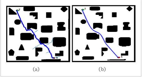
Figure 3
Generated path on a map with inflated obstacles:(a) A generated path using modified goal-biased RRT; (b) An optimized path using A* algorithm
(a) (b)
3.4 Step 4: Path Smoothening
The path obtained after applying A* algorithm (see Figure 3b) is not smooth enough to enable easy navigation of the autonomous vehicle. CSI is employed to enhance the smoothness of the optimized path. With cubic spline, the function of a curve is represented using different cubic functions for each of the data points intervals [3]. Considering m data points, the function of the spline S x( ) can be defined as in Equation (9):
0 1 1 1 1 ( ) ( ) ( ) , ( )
i i i
m m m
x x x
P x
S x P x x x x
P x x −− x x
≤ ≤
= ≤ ≤
≤ ≤
(9) where Pi represents the cubic function. Generally,
cubic spline is defined as:
(7)
where g p( )=c s p( , ) is the path cost c from the initial position s to node p, h(p) is the heuristic component of the cost function which estimates the cheapest cost from node p to the target. h(p) is computed using Eu-clidean distance metric as:
3.3 Step 3: Path Query and Optimization
A path is generated from the initial position of the RRT roadmap to the target using the set of unearest and the T nodes obtained during the generation of the tree. The algorithm used in generating the path is given in Algorithm 2. A sample path generated using Algorithm 2 is demonstrated in Figure 3a. A* algorithm applied in [24] was used to optimize the path in Figure 3a to obtain the path in Figure 3b. In[24], the A* heuristic function was used at every iteration to select the nearest node during the generation of the tree. In this paper, the A* heuristic algorithm is used to optimize and obtain the shortest path after the roadmap is generated using the modified goal-biased RRT. A* heuristic function is good at finding a path on a graph with the least cost provided a path exists [32]. The A* heuristic cost function employed is represented as:
( ) ( ) ( ),
f p =g p h p+ (7)
where g p( )=c s p( , ) is the path cost c from the initial position s to node p, h(p) is the heuristic component of the cost function which estimates the cheapest cost from node p to the target. h(p) is computed using Euclidean distance metric as:
2 2
( ) ( p target) ( p target)
h p = x −x + y −y , (8)
where p=( , , ,..., )p p p0 1 2 pn represents points on the path.
A* is considered because it is both complete and optimal. It is complete as once a path exists in the
free
CS , A* can find the path. A* is admissible and consistent. Admissibility and consistency are properties of optimality. With g(p) being the actual cost to get to point p, f(p) would therefore not overestimate the cost to reach the target. This makes A* admissible. Considering c(p, p') as the cost from point p to p’, consistency is achieved since h p( )≤c p p( , ')+h p( ') and admissibility is achieved since for all arcs of the path,
( , ') 0
c p p ≥ >ε .
Algorithm 2
Path query and optimization algorithm
Input: unearest, T, targetfrom Algorithm 1
Output: apath 1. Begin
2. p←target
3. for j←1to size u( nearest)
4. previous←unearest( )j
5. while j>0
6. p←( (T previous p); )
7. end while
8. end for
9. apath← f p( ) // Equation (7) 10 spath←P apath( ) // Equation (11) 11. End
Figure 3
Generated path on a map with inflated obstacles:(a) A generated path using modified goal-biased RRT; (b) An optimized path using A* algorithm
(a) (b)
3.4 Step 4: Path Smoothening
The path obtained after applying A* algorithm (see Figure 3b) is not smooth enough to enable easy navigation of the autonomous vehicle. CSI is employed to enhance the smoothness of the optimized path. With cubic spline, the function of a curve is represented using different cubic functions for each of the data points intervals [3]. Considering m data points, the function of the spline S x( ) can be defined as in Equation (9):
0 1 1 1 1 ( ) ( ) ( ) , ( )
i i i
m m m
x x x
P x
S x P x x x x
P x x −− x x
≤ ≤
= ≤ ≤
≤ ≤
(9)
where Pi represents the cubic function. Generally,
cubic spline is defined as:
(8)
where p=( , , ,..., )p p p0 1 2 pn represents points on the path.
Algorithm 2
Path query and optimization algorithm
Figure 3
Generated path on a map with inflated obstacles:(a) A generated path using modified goal-biased RRT; (b) An optimized path using A* algorithm
3.3 Step 3: Path Query and Optimization
A path is generated from the initial position of the RRT roadmap to the target using the set of unearest
and the T nodes obtained during the generation of the tree. The algorithm used in generating the path is given in Algorithm 2. A sample path generated using Algorithm 2 is demonstrated in Figure 3a. A* algorithm applied in [24] was used to optimize the path in Figure 3a to obtain the path in Figure 3b. In[24], the A* heuristic function was used at every iteration to select the nearest node during the generation of the tree. In this paper, the A* heuristic algorithm is used to optimize and obtain the shortest path after the roadmap is generated using the modified goal-biased RRT. A* heuristic function is good at finding a path on a graph with the least cost provided a path exists [32]. The A* heuristic cost function employed is represented as:
( ) ( ) ( ),
f p =g p h p+ (7)
where g p( )=c s p( , ) is the path cost c from the initial position s to node p, h(p) is the heuristic component of the cost function which estimates the cheapest cost from node p to the target. h(p) is computed using Euclidean distance metric as:
2 2
( ) ( p target) ( p target)
h p = x −x + y −y , (8)
where p=( , , ,..., )p p p0 1 2 pn represents points on
the path.
A* is considered because it is both complete and optimal. It is complete as once a path exists in the
free
CS , A* can find the path. A* is admissible and
consistent. Admissibility and consistency are properties of optimality. With g(p) being the actual cost to get to point p, f(p) would therefore not overestimate the cost to reach the target. This makes A* admissible. Considering c(p, p') as the cost from point p to p’, consistency is achieved since h p( )≤c p p( , ')+h p( ') and admissibility is achieved since for all arcs of the path,
( , ') 0 c p p ≥ >ε .
Algorithm 2
Path query and optimization algorithm
Input: unearest, T, targetfrom Algorithm 1
Output: apath
1. Begin
2. p←target
3. forj←1to size u( nearest)
4. previous←unearest( )j
5. while j>0
6. p←( (T previous p); )
7. end while
8. end for
9. apath← f p( ) // Equation (7) 10 spath←P apath( ) // Equation (11)
11. End
Figure 3
Generated path on a map with inflated obstacles:(a) A generated path using modified goal-biased RRT; (b) An optimized path using A* algorithm
(a) (b)
3.4 Step 4: Path Smoothening
The path obtained after applying A* algorithm (see Figure 3b) is not smooth enough to enable easy navigation of the autonomous vehicle. CSI is employed to enhance the smoothness of the optimized path. With cubic spline, the function of a curve is represented using different cubic functions for each of the data points intervals [3]. Considering m data points, the function of the spline S x( ) can be defined as in Equation (9):
0 1 1 1 1 ( ) ( ) ( ) , ( )
i i i
m m m
x x x P x
S x P x x x x P x x −− x x
≤ ≤
= ≤ ≤
≤ ≤
(9)
where Pi represents the cubic function. Generally,
cubic spline is defined as:
3.3 Step 3: Path Query and Optimization
A path is generated from the initial position of the RRT roadmap to the target using the set of unearest
and the T nodes obtained during the generation of the tree. The algorithm used in generating the path is given in Algorithm 2. A sample path generated using Algorithm 2 is demonstrated in Figure 3a. A* algorithm applied in [24] was used to optimize the path in Figure 3a to obtain the path in Figure 3b. In[24], the A* heuristic function was used at every iteration to select the nearest node during the generation of the tree. In this paper, the A* heuristic algorithm is used to optimize and obtain the shortest path after the roadmap is generated using the modified goal-biased RRT. A* heuristic function is good at finding a path on a graph with the least cost provided a path exists [32]. The A* heuristic cost function employed is represented as:
( ) ( ) ( ),
f p =g p h p+ (7)
where g p( )=c s p( , ) is the path cost c from the initial position s to node p, h(p) is the heuristic component of the cost function which estimates the cheapest cost from node p to the target. h(p) is computed using Euclidean distance metric as:
2 2
( ) ( p target) ( p target)
h p = x −x + y −y , (8)
where p=( , , ,..., )p p p0 1 2 pn represents points on
the path.
A* is considered because it is both complete and optimal. It is complete as once a path exists in the
free
CS , A* can find the path. A* is admissible and
consistent. Admissibility and consistency are properties of optimality. With g(p) being the actual cost to get to point p, f(p) would therefore not overestimate the cost to reach the target. This makes A* admissible. Considering c(p, p') as the cost from point p to p’, consistency is achieved since h p( )≤c p p( , ')+h p( ') and admissibility is achieved since for all arcs of the path,
( , ') 0 c p p ≥ >ε .
Algorithm 2
Path query and optimization algorithm
Input: unearest, T, targetfrom Algorithm 1
Output: apath
1. Begin
2. p←target
3. forj←1to size u( nearest)
4. previous←unearest( )j
5. while j>0
6. p←( (T previous p); )
7. end while
8. end for
9. apath←f p( ) // Equation (7) 10 spath←P apath( ) // Equation (11)
11. End
Figure 3
Generated path on a map with inflated obstacles:(a) A generated path using modified goal-biased RRT; (b) An optimized path using A* algorithm
(a) (b)
3.4 Step 4: Path Smoothening
The path obtained after applying A* algorithm (see Figure 3b) is not smooth enough to enable easy navigation of the autonomous vehicle. CSI is employed to enhance the smoothness of the optimized path. With cubic spline, the function of a curve is represented using different cubic functions for each of the data points intervals [3]. Considering m data points, the function of the spline S x( ) can be defined as in Equation (9):
0 1 1 1 1 ( ) ( ) ( ) , ( )
i i i
m m m
x x x P x
S x P x x x x P x x −− x x
≤ ≤
= ≤ ≤
≤ ≤
(9)
where Pi represents the cubic function. Generally,
cubic spline is defined as:
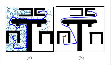
![Figure 13 To aid in comparing the efficiency of the proposed method to RRT-A*, experiments are performed us-ing the maps used in [24]](https://thumb-us.123doks.com/thumbv2/123dok_us/8763577.1753271/11.595.67.292.334.468/figure-comparing-efficiency-proposed-method-rrt-experiments-performed.webp)