Volume 16, Number 4, pp. 403–421. http://www.scpe.org
ISSN 1895-1767 c
⃝2015 SCPE
MULTI-OBJECTIVE DISTRIBUTED CONSTRAINT OPTIMIZATION USING SEMI-RINGS
GRAHAM BILLIAU∗, CHEE FON CHANG†, AND ADITYA GHOSE‡
Abstract. In this paper, we extend the Support Based Distributed Optimization (SBDO) algorithm to support problems which do not have a total pre-order over the set of solutions. This is the case in common real life problems that have multiple objective functions. In particular, decision support problems. These disparate objectives are not well supported by existing Dis-tributed Constraint Optimization Problem (DCOP) techniques, which assume a single cost or utility function. As a result, existing Distributed COP techniques (with some recent exceptions) require that all agents subscribe to a common objective function and are therefore unsuitable for settings where agents have distinct, competing objectives. This makes existing constraint optimization technologies unsuitable for many decision support roles, where the decision maker wishes to observe the different trade-offs before making a decision.
Key words: Multi-objective Optimisation, Constraints, Semi-Rings.
AMS subject classifications. 65K10, 97H40
1. Introduction. The simple approach of modelling DCOPs, where the cost/utility of a solution is mea-sured as a single real number, is quite restrictive. This approach can only represent problems where there is a total pre-order over the solutions. Many real world problems only have a partial order over the solutions. Examples of these problems include problems with multiple objectives and problems with qualitative valuations. To further complicate things, a problem may include a mix of qualitative and quantitive valuations.
Bistarelli’s c-semiring framework [3] is very successful for modelling problems in the Constraint Optimisation Problem (COP) domain. The Distributed Constraint Optimisation Problem (DCOP) domain introduces several new modelling challenges over centralised problems. These challenges include agent responsibility, privacy, co-operating/competing agents and no global objective. Further, these challenges lead to classes of DCOP problems which have not been addressed in the literature so far. The existing modelling frameworks do not support these new classes of problems, so we are proposing a new modelling framework inspired by c-semirings.
We have identified three classes of problems within the DCOP domain which can not be adequately de-scribed using c-semirings; equitable problems, maximisation problems and ‘committee’ problems. For equitable problems, we specifically refer to problems with an objective of the form ‘minimise the maximum difference between the best and worst criteria’. Examples of these problems include distributing rewards to a team, as-signing jobs to workers and minimise the impact of flood mitigation. Some examples of maximisation problems include maximise profit within a supply chain, maximise the value of targets tracked in a sensor network and maximise the area a team of drones can search. Committee problems are when a group of agents must agree on one (or more) shared decisions. This includes problems such as deciding on a requirements specification or a CEO’s bonus package.
Equitable problems are particularly interesting within a distributed system. This is because there may not be a single ‘dictator’ agent who defines the entire problem. Instead the problem may grow organically, as individual agents discover they share a common goal and agree to limited co-operation. While the agents may loosely agree on the common goal, each agent has other goals, which may conflict. The end result is that there may not be a single objective which all agents subscribe to. Further, individual agents may be selfish or altruistic, which determines how much weight they put on their local objectives. In these cases, a compromise (such as an equitable solution) is required.
Equitable problems often occur in the medical setting, where the objective is to balance the patients quality of life and their survival chances. To do this, the doctor must find a balance between the most aggressive treatment (maximum survival chances, minimal quality of life) and the least aggressive treatment (minimal
∗Decision Systems Lab, University of Wollongong, NSW, Australia ([email protected])
†Centre for Oncology Informatics, University of Wollongong, NSW, Australia ([email protected]) ‡Decision Systems Lab, University of Wollongong, NSW, Australia ([email protected])
survival chances, maximum quality of life). Two examples of this include treating larynx cancer and methicillin-resistant staphylococcus aureus. Radiotherapy is an effective way to treat larynx cancer, but at high doses paralyses the patient’s vocal cords. Similarly, amputation is the most effective way to treat staph infections, but then the patient looses the affected limb.
One possible way to represent an equitable problem is using a tuple of n real numbers to represent the utility for each agent. This can be represented using the semiring ⟨ℜ × ℜ × · · · × ℜ,⊕,⊗⟩. The objective is to minimise the difference between the highest and lowest values in the tuple. Defining the ⊕operator as follows captures this idea.
⊕(A, B) =
{
A if (max(A)−min(A))≤(max(B)−min(B))
B otherwise
whereA=⟨a1, a2, . . . , an⟩andB=⟨b1, b2, . . . , bn⟩are tuples of real numbers, so max(x) and min(x) return the
largest or smallest value in the tuple respectively. The real numbers represent utility, so to get the total utility for an agent, the individual utilities are added together.
⊗(A, B) =⟨a1+b1, a2+b2, . . . , an+bn⟩
This problem can’t be represented as a c-semiring. A c-semiring requires a ⊤ value which is the absorbing element of ⊕ and the unit element of ⊗. It also requires a ⊥value which is the unit element of ⊕ and the absorbing element of ⊗. In this problem, there does not exist a unique ‘best’ value to use as ⊤ or a unique ‘worst’ value to use as⊥.
Egalitarian problems, a more common class of problems with a similar intuition also can’t be represented as a c-semiring. By an egalitarian problem we specifically refer to problems with the objective “maximise the minimum utility” or “minimise the maximum cost”. In these problems there is still no unique best or worst value. So long as one of the values is∞, then any assignment to the other values will compare as the equal best (or worst) value. To represent such a problem using a c-semiring, the objective must be defined as “minimse the maximum cost, then minimise the next highest cost, ... then minimise the lowest cost”. This objective still satisfies “minimise the maximum cost”, though it also considers the other values.
Maximisation problems are often represented using valued constraints. They can also be represented using the semiring ⟨ℜ,max,+⟩. These problems can’t be directly represented as c-semirings, as ∞is the absorbing element for both max and +. In centralised settings, maximisation problems are commonly transformed into minimisation problems (represented by the c-semiring ⟨ℜ+0,min,+,0,∞⟩). This transformation involves first mapping ℜtoℜ−0 by subtracting∞, then changing it to a minimisation problem by multiplying all the values by −1. Performing this transformation in practice requires knowing the maximum possible utility value. In dynamic or distributed settings, this is not possible. For dynamic settings, changes to the problem may result in a larger maximum possible utility value. For distributed settings, computing the largest possible utility value requires complete knowledge of the problem, which violates one of the assumptions of distributed problems. As the transformation is not applicable in these settings, the framework has to support the maximisation problem directly.
Finally we consider committee problems. This is a class of problems where a group of agents must agree on the answer to one (or several) decisions. Committee problems can be modelled as a standard DCOP by arbitrarily assigning agents control of decisions (variables). They could be modelled much more elegantly if agents are allowed to share control of variables. Problems of this form are usually modelled and solved as negotiation problems. If the committee problem is a sub-problem of a larger optimisation problem, then solving the larger problem requires a hybrid DCOP/negotiation algorithm or modelling the entire problem as a DCOP. Further, negotiation algorithms generally assume competitive agents, while for this work we assume cooperative, though not trusting, agents.
We present a simple requirements engineering problem as an example of a committee problem. There are ncandidate requirements (the variables,X), which have been identified during the requirement elicitation process. Each candidate requirement can either be included (True) or excluded (False) from the specification (the domains, D1, . . . , Dn). In addition, there aremstakeholders (the agents, A), each of whom has different
preferences for which candidate requirements should be included (the constraints, C). Finally, the objective is to maximise the total utility of the stakeholders (maximisation problem,V).
In this setting all of the stakeholders know all of the candidate requirements and may propose a value for any of them. The stakeholders would like to keep their preferences private. Modelling this as a traditional DCOP problem would require arbitrarily assigning stakeholders control over the candidate constraints. Further, if we assume that each stakeholder has preferences regarding most of the constraints, then they will be forced to reveal their preferences to most of the other stakeholders. This is because most DCOP solvers require all agents involved in the constraint must know the details of the constraint. Recent work on asymmetric constraints [8] goes some way towards addressing this concern. By allowing multiple agents to share control of variables, this problem can be modelled naturally. The resulting model is also better at maintaining each agent’s privacy.
These classes of problems may overlap, as shown in the following example. There are two agents {1, 2} sharing control of two variables{X, Y} with the same domain{−1,0,1}. The global objective is that the sum of the variables should be zero. Agent 1’s objectives are to maximise X and minimise Y. Agent 2’s objectives are to minimise X and maximise Y.
The (utilitarian) optimal solutions for this problem are: • X = 1, Y =−1 (In favour of Agent 1)
• X =−1, Y = 1 (In favour of Agent 2) There is one equitable solution:
• X = 0, Y = 0 (balance between both Agents)
A utilitarian solver will likely not return the equitable solution as a possible solution. While the equitable solution satisfies the global objective, it does not satisfy either of the local objectives.
In section 2 we describe the framework which we propose to model these classes of problems. Next we show the relationship between our framework and some of the established frameworks in section 2.3. We then detail an algorithm designed to solve problems expressed using this framework in section 3 and show the performance of the algorithm in section 4. Finally the conclusion summarises our contribution.
2. Semiring-based Distributed Constraint Optimization Problems. In this section, we will intro-duce our proposed framework, the Semiring-based Distributed Constraint Satisfaction/Optimization Problem (SDCOP). The proposed framework draws inspiration from Bistarelli et al. [3]. As such, there exists many com-monalities. Bistarelli et al. [3] proposed the use of a c-semiring for comparing different solutions. The original formulation of a c-semiring was for use within the CSP domain. We view this approach to be too restrictive for use within the CSOP domain. Specifically, a c-semiring does not support optimization problems where the objective is to maximize utility. Objective functions of this form are required for some recent algorithms (specifically SBDO [2]). Thus, we propose the use of an idempotent semiring. The use of the semiring structure allows for two main benefits. Firstly, in multi-objective problems where no total pre-order over the solutions are prescribed, the use of an abstract structure (i.e. semirings) allows the framework to induce a partial ordering. Secondly, using an abstract comparison and aggregation operators allows the framework to support comparison and combination across both qualitative and quantitative domains.
2.1. Preliminaries: Idempotent Semirings. A semiring consists of a set of abstract values and two operators. The two operators allows for the comparison and combination of the prescribed abstract values.
Definition 2.1. A semiring[17] is a tupleV =⟨V,⊕,⊗⟩ satisfying the following conditions: • V is a set of abstract values.
• ⊕is a commutative, associative and closed operator overV. • ⊗is an associative and closed operator over V.
• ⊗left and right distributes over ⊕.
We shall call a semiring an idempotent semiringif ⊕is idempotent.
• ⊕is defined over possibly infinite sets as follows: – ∀v∈V,⊕({v}) =v
– ⊕(∅) =⊥and⊕(V) =⊤ – ⊕(∪v
i, i∈S) =⊕({⊕(vi), i∈S})for all sets of indicesS
• ⊗ is a commutative, associative and closed binary operator onV with ⊤as unit element (α⊗ ⊤=α) and⊥as absorbing element (α⊗ ⊥=⊥).
• ⊗distributes over ⊕(i.e.,α⊗(β⊕γ) = (α⊗β)⊕(α⊗γ)).
The idempotent property of the⊕operator can be used to obtain a partial order≼V over the set of abstract values V. Such a partial order is defined as: ∀(v1, v2 ∈ V), v1 ≼V v2 iff v1⊕v2 = v1 (intuitively, v1 ≼V v2
denotes thatv1is at least as preferred asv2). The⊕operator enables comparisons between two semiring values
while the⊗operator allows us to aggregate two semiring values.
This idempotent semiring structure is now capable of representing all the different constraint schemes. As a c-semiring is an idempotent semiring, all constraint schemes that can be represented as c-semirings can also be represented as idempotent semirings.
Bistarelli has shown that classic, fuzzy, probabilistic, weighted and set based constraints are all instances of a c-semiring [3]. Valued constraints with a maximization objective are not an instance of a c-semiring, but can be represented by the idempotent semiring⟨ℜ,max,+⟩whereℜis the set of values, max is the comparison operator and + is the combination operator.
Multiple idempotent semirings may be combined into a single idempotent semiring in the same way that c-semirings are combined [3]. The semirings being combined may involve evaluations on multiple heterogeneous scales - both qualitative and quantitative. We leverage this property in handling multi-objective DCOPs.
The following definition is based on that provided by Bistarelli et. al [3] (definition 7.1) for c-semiring. It formalizes the combination of idempotent semirings.
Definition 2.3. Given the n idempotent semirings Si = ⟨Vi, ⊕i, ⊗i,⟩ for i = 1, . . . , n we define the structure Comb(S1, . . . , Sn) = ⟨⟨V1, . . . , Vn⟩, ⊕, ⊗⟩ where ⊕ and⊗ are defined as follows: Given ⟨a1, . . . , an⟩
and⟨b1, . . . , bn⟩such thatai, bi∈Vi fori= 1, . . . , n,⟨a1, . . . , an⟩ ⊕ ⟨b1, . . . , bn⟩=⟨a1 ⊕1 b1, . . . , an⊕nbn⟩and ⟨a1, . . . , an⟩ ⊗ ⟨b1, . . . , bn⟩=⟨a1 ⊗1 b1, . . . , an⊗nbn⟩.
Theorem 2.4. If Si=⟨Vi, ⊕i, ⊗i⟩ fori= 1, . . . , n are all idempotent semirings, thenComb(S1, . . . , Sn)
is an idempotent semiring.
Proof. From definition 2.3, the combined semiring uses the⊕and⊗operators from the component semirings directly. Hence, the properties that hold for the component semirings also hold for the combined semiring.
If a⊕b = a then for all components i, ai⊕ibi = ai. This corresponds to the ‘dominates’ concept in pareto-optimality. Hence the Comb() operator implements the commonly accepted pareto-optimal ordering over multiple objectives. If a different ordering is desired then the⊕ operator can be redefined to implement the desired ordering.
A unified formulation must also support the concept of agents. The concept of agents is required for distributed problems. An agent has knowledge of a subset of the entire problem and can only affect a subset of the sub-problem it knows. There are several common justifications (such as resource limits, privacy concerns and communication capacity) for limiting an agent’s knowledge to only a subset of the entire problem. Furthermore, resource and communication limitations can lead to efficiencies, such as a reduction of memory requirements for each agent and a reduction in required messages to keep the knowledge of all agents synchronized. An agent may also not know of variables and constraints that represent privileged information held by another agent.
Definition 2.5. A Semiring-Based Distributed Constraint Satisfaction/Optimization Problem (SDCOP) is a tuple ⟨A,X,D,V,C⟩where
• A is a non-empty set of agents. An agent is a pair α=⟨Rα, Wα⟩. Ra is a set of variables for which the agent has read privileges, and Wα ⊆ Rα is a set of variables for which the agent has write privileges.
• X is a set of variables.
• D is a set{D1, . . . , Dn} where n=|X |and each Di is a set of values to be assigned to a variable (the domain).
• V =⟨V,⊕,⊗⟩ is an idempotent semiring utilized to evaluate variable assignments.
• C is a non-empty set of constraints, where each constraint ci is a pair ⟨defi, coni⟩ where defi is a function defi : (∪D)k −→V (wherek=|coni|) andconi⊆ X is thesignature of constraintci (i.e., the set of variables referred to in that constraint).
If an agent α has write privileges for a variablev,αmust also have read privileges for all variables which share a constraint with v i.e. ∀v∈Wα,∀ci∈ C, ifv∈coni, thenconi⊂Rα.
The set of agents refers to the agents that must co-operate to solve the problem. There is of course much more to an agent than just its privileges, such as the amount of resources available or the ‘temperament’ of the agent. We do not consider those attributes (and similar ones) of agents as they only apply to solving the problem, not to the description of the problem.
Read privileges serve a dual purpose. The primary purpose is to identify which agents must know the value assigned of a variable. The secondary purpose is to determine the required communication links between agents. Knowledge of variable assignments is only one aspect of privacy. Often it is also desirable to ensure that other agents can not discover the constraints on an agent’s variables. The flow of such information is entirely dependent on the algorithm and so is outside the scope of this work.
As the required communication is already prescribed by read privileges, the write privileges are purely to determine which agents have permission to allocate a value to a variable. In most situations, it is acceptable for there to be variables in the problem for which no agent has write privileges. These can be viewed as hard constraints or environmental constants. This concept is particularly useful in a mixed-initiative setting whereby assignments made by the human operator should not and cannot be overruled by the machine solver.
The explicit assertion of read/write privileges is unique to this formulation. Traditional formulations im-plicitly prescribe global read privileges while maintaining only local write privileges. We feel that this approach over simplifies real world problems. Such an assumption creates additional communication overhead to main-tain synchronization and impedes on the scalable and distributed nature of DCSOPs. Furthermore, to honestly reflect the privacy property in DCOPs, the read/write privileges prescribes access control machinery to control access to information. However, note that the traditional formulation (global read/local write) approach is a special case for our formulation where agents are given read privileges to all variables. It also allows for param-eters (variables for which no agent has write access) to be naturally represented within the problem and allows the community to explore problems without the simplifying assumption that agents have exclusive control over variables. Designing algorithms which support allowing multiple agents to write to a variable presents new challenges. The algorithm must have some mechanisim for either managing access to the variable or resolving the resulting inconsistancies.
communication channels between agents exist only in situations where the agents share variables. More formally,
Definition 2.6. Given a SDCOP=⟨A,X,D,V,C⟩, a neighbourhood graphis a directed graph⟨N, E⟩ whereN =AandE⊆ A×Asuch that∀α, α′∈ A,⟨α, α′⟩ ∈Eiffα̸=α′∧∃x∈ X such thatx∈W
α∧x∈Rα′.
If an agentαhas write privileges to a variablexand another agentα′has read privileges toxthen they must
be able to communicate, as αmust informα′ of any changes it makes tox. If two agents must communicate
then they are in the same neighbourhood.
Variables are identified by a unique name. All variables share the same domain, rather than having separate domains as per common practice. The common domain can be viewed as the union of all individual domains, with unary constraints on the individual variables restricting which subset of the domain values can be assigned to the variables. This approach generalizes existing practice. The idea of having the domain of each variable defined by unary constraints was discussed by Ross et. al. [18]
Our use of functions that return a value from an idempotent semiring allows for the representation of a range of different forms of constraints. In classic satisfaction problems, the semiring ⟨{True,False},∨,∧⟩is sufficient to reflect the satisfaction of the constraints. For valued constraint optimization problems, the semiring ⟨ℜ,min,+⟩is suitable for minimization problems and⟨ℜ,max,+⟩is suitable for maximization problems. In the cases where there are multiple objective functions, each objective is represented by its own idempotent semiring. TheComb() operator can then be utilized to combine the individual semirings. Using this approach to combine the different objectives naturally leads to a search for a pareto-optimal solution. By using this approach we do not impose an ordering on the objectives, however an ordering can be added if so desired. Furthermore, such an approach also allows for all the different types of constraints to be combined.
We also distinguish between two classes of constraints: local constraints and shared constraints. A local constraint is known by only one agent and can only be evaluated by that agent. For this to occur one agent must have write privileges to all of the variables inconi (refer to definition 2.5). Shared constraints are known by all agents which have write privileges to a variable in the constraints signature and can be evaluated by any one of those agents. This occurs when more than one agent has write privileges to one of the variables in coni (refer to definition 2.5).
Definition 2.7. Given an SDCOP ⟨A,X,D,V,C⟩, S is the set of all possible assignments to variables. Each assignment is a set of variable-value pairs where no variable appears more than once. We will refer to an assignments∈ S as acomplete assignmentif it assigns a value to every variable inX. For some assignment
s∈ S, we will use s↓X to denote the projectionof the assignment to a set of variablesX (i.e., the subset ofs
that refers to variables inX). Given an assignments=⟨⟨x1, v1⟩,⟨x2, v2⟩, . . . ,⟨xk, vk⟩⟩,val(s) =⟨v1, v2, . . . , vk⟩
andvar(s) =⟨x1, x2, . . . , xk⟩.
The different criteria are reflected in the definition of a solution to a SDCOP. The concept of a solution to a satisfaction problem is generalized in our definition of an acceptable solution.
Recall that our unified definition of a CSP is agnostic to the solving method, so while it has been shown [16] that combining semirings is not sufficient for solving multi-objective problems using inference based methods [1, 5, 6, 7, 15] (specifically the operators ⊕
and ⊗
). However, combining semirings is sufficient for search based methods [2, 20], which are common in the DCOP literature. For this reason we define the solutions to a SDCOP in terms of the properties they must satisfy, which are independent of the solving method and the semiring used to evaluate assignments. Furthermore, we utilize a notion of acceptable threshold to define an acceptable solution to an optimization problem. The idea of an acceptable threshold on an optimization problem has been proposed by J. Larrosa [11].
Definition 2.8. An acceptable solutionto a SDCOP with C={c1, . . . , cn}is a complete assignment s
such that def1(val(s↓con1))⊗. . .⊗defn(val(s↓conn))≼V v, wherev∈V is a minimum threshold on the value
of the solution.
The solution to a classic satisfaction problem can be represented as an acceptable solution with a threshold of True. An acceptable solution is also useful to represent problems where the optimal solution is not required or it is too expensive to search for the optimal solution.
Definition 2.9. An optimal solution to a SDCOP with C = {c1, . . . , cn} is a complete assignment s
such that there does not exist another complete assignments′ wheredef
1(val(s′↓con1))⊗. . .⊗defn(val(s′↓conn
Theorem 2.10. At least one optimal solution exists for any SDCOP.
Proof. The associative property of⊕means that the ordering≼V derived from⊕is transitive. Due to the ordering being transitive, cycles can not exist within the ordering. Because there are no cycles there must be at least one abstract value which is not dominated by another abstract value.
The constraints map each assignment to exactly one abstract value, which is used to order the assignments. As such, the ordering over assignments is also transitive. Therefore there must be at least one complete assignment which is not dominated by another complete assignment.
Note that the definition of an optimal solution is equivalent to a non-dominated solution, as such the set of all optimal solutions is the pareto-frontier. If an acceptable solution (for a given threshold) does not exist, one way to get a solution which is acceptable is to relax the concept of a solution. This is done by not requiring a complete solution to the SDCOP.
Definition 2.11. Given a constraint ci = ⟨defi, coni⟩ the projection of ci onto a set of variables X,
ci↓X=⟨defi′, coni∩X⟩. Ifconi⊆X thenci is returned unchanged. defi′ is defined such that for a given input
V it returns one of the values defi can return for the inputV expanded to include values for the other variables in coni.
There are two different intuitions about which value to return in the projected version of the constraint. First, the projected constraint should return the best possible value using the assigned variables. Second, the projected constraint should return the worst possible value using the assigned variables. It is possible that there is more that one best or worst value, as the semiring allows a partial ordering. In this case the choice between the best or worst values is arbitrary.
Definition 2.12. Given a set of constraints C = {c1, . . . , cn} and an assignment s, let C′ ={c1 ↓var(s) , . . . , cn ↓var(s)}. s is a relaxed solution with reference to the constraints C′ iff def1(val(s ↓con1))⊗. . .⊗ defn(val(s↓conn))≼V v, wherev is a minimum threshold on the value of the solution and there does not exist
another assignment s′ where|s′|>|s| anddef
1(val(s′ ↓con1))⊗. . .⊗defn(val(s
′ ↓con
n))≼V v.
There are many other ways to define a solution to a SDCOP, such as ak-optimal solution [13]. These other solution concepts can be easily modified for the SDCOP structure.
2.3. Example Instantiations. In this section, we will illustrate the usefulness of our framework by the SDCOP instances that correspond to several common DCOPs. We will do so by presenting three instantiations: a CSP instance, a DCOP instance and a DCOP variation. Bistarelli’s c-semiring framework [3] is one of the commonly accepted frameworks for generalizing CSP problems. Both Bistarelli’s c-semiring framework and our SDCOP framework are based on using a variation of a semiring to order the solutions. As highlighted earlier, CSPs are special instances of DCOPs. Hence, it is befiting to illustrate the generality of SDCOP by demonstrating Bistarelli’s c-semiring framework is a special instance of an SDCOP.
Theorem 2.13. Any problem represented as a c-semiring can be represented as an idempotent semiring. Any idempotent semiring which also satisfies the following properties can be represented as a c-semiring.
• ⊥i∈V is the absorbing element of⊗and the unit element of⊕. • ⊤i∈V is the unit element of⊗and the absorbing element of⊕.
Proof. We consider two representations of a constraint optimisation problem to be equivalent iff the solutions of the representations are equal. The solution to a constraint optimisation problem is defined in terms of the⊕ and ⊗operators. Therefore it is sufficient to show that the⊕and⊗operators in c-semirings and idempotent semirings have the same properties.
Given a c-semiring⟨Vc,⊕c,⊗c,⊥c,⊤c⟩and an idempotent semiring⟨Vi,⊕i,⊗i,⊥i,⊤i⟩as described above, we show that the two are equivalent.
Vi and Vc are equivalent by definition, as are ⊗i and ⊗c. ⊥i,⊥c are the absorbing elements of ⊗i,⊗c respectively, as per the definition. Similarly ⊤i,⊤c are the unit elements of⊗i,⊗c respectively.
We have just shown that the idempotent semiring used in our framework is more general than the c-semiring used in Bistarelli’s framework [3]. Therefore, all the constraint schemes which can be represented in Bistarelli’s framework can also be represented in our framework. Namely classical, fuzzy, probabilistic, weighted (minimization), set based, and multi-objective constraint optimization problems.
There exists several formulations of DCOPs [2, 7, 12, 14, 20]. All of these formulations capture the important aspects of DCOPs equally well. We will focus on the instantiation of Petcu’s formulation [14] into SDCOP as it is the most formal definition.
Petcu [14] defines a COP as follows:
Definition 2.14. [14] Adiscrete constraint optimization problem (COP) is a tuple⟨X,D,R⟩ such that: • X ={X1, . . . , Xn} is a set ofvariables (e.g. start times of meetings);
• D={d1, . . . , dn} is a set of discrete, finite variable domains(e.g. time slots);
• R={r1, . . . , rm} is a set ofutility functions, where eachri is a function with the scope(Xi1, . . . , Xik), ri :di1 × · · · ×dik −→ ℜ. Such a function assigns a utility (reward) to each possible combination of
values of the variables in the scope of the function. Negative amounts mean costs. Hard constraints (which forbid certain value combinations) are a special case of utility functions, which assign0to feasible tuples, and −inf to infeasible ones;
Definition 2.15. [14] A discrete distributed constraint optimization problem (DCOP) is a tuple of the following form: ⟨A,COP,Ria⟩such that:
• A={A1, . . . , Ak} is a set of agents (e.g. people participating in meetings);
• COP ={COP1, . . . , COP} is a set of disjoint, centralized COP s; each COPi is called the local sub-problem of agent Ai, and is owned and controlled by agent Ai;
• Ria={r
1, . . . , rn} is a set of inter-agent utility functions defined over variables from several different
local sub-problems COPi. Eachri :di1× · · · ×dik −→ ℜexpresses the rewards obtained by the agents
involved inrifor some joint decision. The agents involved in ri have full knowledge ofri and are called ‘responsible’ forri. As in a COP, hard constraints are simulated by utility functions which assign 0 to feasible tuples, and −∞to infeasible ones;
Further, Petcu defines a solution as:
Definition 2.16. [14] The goal is to find a complete instantiationX for the variables Xi thatmaximizes the sum of utilities of individual utility functions. The definition of a solution provided by Petcu [14] corresponds to the definition of an optimal solution within SDCOP. This definition of a DCOP corresponds to the following SDCOP:
Theorem 2.17. Petcu’s definition of a DCOP is a SDCOP⟨A,X,D,V,S,C⟩with the additional properties: • Exactly one agent has write access for each variable.
• ∪
D is finite. • V =⟨ℜ,max,+⟩.
Proof. The two formulations are equivalent iff every problem that can be described by Petcu’s definition has an equivalent definition within the SDCOP and every problem that can be described by the SDCOP has an equivalent definition within Petcu’s definition.
We start by showing that every problem that can be described by Petcu’s definition has an equivalent definition within the SDCOP. It is clear that both formulations support the concept of agents. Petcu’s definition allows an agent to control a set of variables described as a sub-problem while SDCOP directly specifies the variables that an agent controls. Petcu’s use of real numbers to measure utility can easily be represented by the idempotent semiring⟨ℜ,max,+⟩
entire domain, then propagating all the unary constraints on that variable. The resulting domain is specific domain for that variable. After this the unary constraints can be removed. Restriction three limits SDCOP to using real numbers as the utility, which is equivalent to Petcu’s use of real numbers. Finally the use of n-ary constraints in SDCOP is almost identical to the constraints in Petcu’s definition.
Recently, Grinshpoun et al. proposed the Asymmetrical DCOP (ADCOP) model [8]. In this model, the utility gained by each agent participating in a constraint is tallied separately, however the objective is to minimize (maximize) the sum of the utilities of all agents. The motivation is to preserve the privacy of each agent regarding its local utility. Grinshpoun et al. [8] define a DCOP as follows:
Definition 2.18. [8] A DCOP is a tuple⟨A,X,D,R⟩. Ais a finite set of agentsA1, A2, . . . , An. X is a
finite set of variables X1, X2, . . . , Xm . Each variable is held by a single agent (an agent may hold more than one variable). Dis a set of domainsD1, D2, . . . , Dm. Each domainDi contains a finite set of values which can be assigned to variableXi . Ris a set of relations (constraints). Each constraintC∈R defines a non-negative cost for every possible value combination of a set of variables, and is of the form:
C:Di1×Di2× · · · ×Dik−→ ℜ+ (2.1)
Grinshpoun et al. [8] define an ADCOP as follows:
Definition 2.19. [8] An ADCOP is defined by the following tuple⟨A,X,D,R⟩, where A,X , andDare defined in exactly the same manner as in DCOPs. Each constraint C ∈R of an asymmetric DCOP defines a set of non-negative costs for every possible value combination of a set of variables, and takes the following form:
C:Di1×Di2× · · · ×Dik−→ ℜ+ k
(2.2)
Grinshpoun’s definition of a DCOP is comparable to Petcu’s, which we have already shown to be an instance of of an SDCOP. It remains to show that the constraint definition in an ADCOP is an instance of an idempotent semiring.
Theorem 2.20. Asymmetrical constraints as defined in a ADCOP can be represented as the an idempotent semiring ⟨V,⊗,⊕⟩ where: V is the Cartesian product of the set of utilities for each agent. ℜn
+, given agents a1, . . . , an,⊗is defined as ⊗(v, v′) =⟨v1+v1′, v2+v2′, . . . , vn+vn′⟩and⊕is defined as
⊕(v, v′) = {
v Σ1
nv≤Σ1nv′
v′ otherwise (2.3)
In addition, if there does not exist a variable which is owned by an agent α, in the signature of a constraint c, then the cost forαin the result of the constraintc must be zero.
Proof.
The ADCOP definition allows the cost for each agent to be recorded separately, by having one integer/real number for each agent, the idempotent semiring described also allows the cost for each agent to be recorded separately. The aggregation operator in ADCOP is sum, with the cost for each agent aggregated separately, this is reflected in the ⊗operator. The comparison operator in ADCOP is a utilitarian minimization operator, this is reflected in the ⊕operator.
The idempotent semiring always includes a cost for all agents, even if the agent is not involved in the constraint, thus it may represent constraints that can’t be represented in an ADCOP. The restriction on the cost for an agent if the agent is not part of the constraint prevents this case.
3. Semi-Ring Support Based Distributed Optimisation. The Support Based Distributed Optimisa-tion (SBDO) algorithm [2], which this algorithm extends, is intended to be deployed in real life environments. We characterise real life environments as having the following properties:
• Dynamic • Anarchic
• Hetrogeneous agents • Selfish agents • Malicious agents
These are in addition to the properties of the problem, such as different constraint types and multiple objectives. In order to operate in this environment, we identified three ideals that the algorithm should meet. These are autonomy, equity, and fault tolerance. Autonomy means that the agent retains control of its local knowledge and has the power to act or not act as its situation dictates. Equity means that each agent has the same influence over the final solution and requires a similar amount of resources to the other agents. Fault tolerance means that the overall system should not fail when any of its components fails.
In order to attempt to meet these ideals, SBDO is based on negotiation/argumentation between the agents, rather than a power structure as commonly used. Because of this, the agents have equal power over the other agents and the final solution to the problem. In the process of solving the problem, the agents dynamically form coalitions and use their combined power to influence the other agents. These coalitions are determined based on the structure of the problem and random chance, rather than any bias in the algorithm. The lack of an enforced structure means that the algorithm is not unduly affected should an agent fail, and can continue attempting to solve the problem without the failed agent. The redundancy built into the message passing means that an agent which fails can be recovered quickly. The communication protocol used is also not sensitive to messages arriving in the wrong order. Together these make the algorithm tolerant of a variety of different faults.
The version of SBDO described in this chapter can solve SDCOP problems which meet the following conditions:
• The domain of variables (∪D) must be finite.
• The quality of a solution must be monotonically non-decreasing as the solution is extended, i.e. ∀a, b∈
V, a⊗b≼a.
How SBDO and SBDOsr support dynamic problems is discused in earlier publications [2], so is not discused here.
We start our discussion of the SBDOsr algorithm by defining the messages sent between agents.
Definition 3.1. An assignment is a triple ⟨a, v, u⟩ where a is an agent in the SDCOP, v is a set of variable-value pairs, and u is the utility of this assignment returned by the agents local constraints. v must contain a variable-value pair for every variable inWa for which another agent has read privileges.
Definition 3.2. Given an SDCOP=⟨A,X,D,V,C⟩, aproposalis a pair⟨VA,SCE⟩, where VA (variable assignments) is a sequence ⟨ass1, . . . , assn⟩of assignments such that the sequence of agents forms a simple path
through the neighbourhood graph and there are no conflicting assignments. SCE (shared constraint evaluations) is a set of evaluations of shared constraints. A shared constraint can only be evaluated if an assignment to every variable involved in the constraint is included in VA. Each evaluation is a tuple ⟨o, u⟩whereois a shared objective and uis the utility returned by the objective functiono given the assignments in V A.
As an example, consider the two agents A and B, who share a constraint O, as well as having their own local constraints. When A first creates a proposal it simply contains an assignment to A,⟨⟨⟨A,{⟨a,1⟩},3⟩⟩,{}⟩. Later when B extends the proposal, B then has enough information to evaluate the shared objective, producing ⟨⟨⟨A,{⟨a,1⟩},3⟩,⟨B,{⟨b,2⟩},2⟩⟩,{⟨O,10⟩}⟩.
The sequence of variable assignments indicates the order in which this proposal has been constructed and is required both to store the utility of the solution and for the generation of nogoods. The set of shared constraint evaluations is required to record the utility of constraints shared by more than one agent. If the utility of the shared constraints is combined with the local constraints they might be double counted when cycles form. Note that in situations where privacy is important, the assignment to a variable only needs to be disclosed if another agent has a constraint involving this variable.
The utility value provides a partial order over the the proposals (partial solutions). Comparison between proposals can be performed by first applying the⊗operator over the utility of each assignment and evaluation to determine its utility value and then the ⊕ operator to determine which proposal is better. Whenever we refer to one proposal being better than another in this paper it is with respect to this induced ordering.
The counterpart of a proposal is a nogood. A nogood represents a partial solution that violates at least one constraint and should never be reconsidered or included in the final solution. This inconsistency is discovered when the utility of an isgood is⊥. Nogoods with justifications [19] are used as these allow us to guarantee that all the hard constraints are satisfied (as shown in [10]) as well as allowing obsolete nogoods to be identified after the constraints that the nogood violated are removed from the problem. For our purposes, a nogood with justification (originally defined in [19]) is treated as follows:
Definition 3.3. Given an SDCOP⟨A,X,D,V,C⟩, anogoodis a pair⟨P, C⟩whereP is a set of variable-value pairs representing a partial solution and C ⊆ C is the set of constraints that provides the justification for the nogood, such that the combination of sandC is inconsistent (results in ⊥).
A minimal nogood is a nogood n =⟨P, C⟩ such that there does not exist a nogood n′ =⟨P′, C⟩ where
P′⊂P or a nogoodn′′=⟨P, C′⟩where C′ ⊂C.
In static environments, detecting that the network has reached a quiescent state is sufficient to detect termination. This can be achieved by taking a consistent global snapshot [4]. The algorithm will also terminate if it detects that there is no solution to the problem, by generating the empty nogood. Otherwise, due to the dynamic nature of the input problem, the algorithm will only terminate when instructed to by an outside entity. Detecting that the network of agents has reached a quiescent state, or detecting that the problem is over-constrained are in themselves insufficient as terminating criteria, since new inputs from the environment, in the form of added or deleted variables/constraints might invalidate them.
Algorithm 1send nogood(I) Let N be a nogood derived from I Send N to A
Delete I
Algorithm 2process remove-nogood message Let C be the constraint referenced
forEach received nogood Ndo
if N is in the remove-nogood message then Delete N fromnogoods
delete N from the remove-nogood message if counter̸= 0then
Add the remove-nogood message toremoved-constraints receive remove constraint(C)
3.1. Algorithm. The core of SSBDO is very simple. First the agent reads any messages it has received from other agents and updates its knowledge. If it has received a proposed solution from another agent that is inconstant, it responds with a nogood message. Second it chooses an assignment for all variables for which it has write privileges. Third the agent sends a message to each of its neighbours, informing them of any change to its proposals. Finally the agent waits until it receives new messages.
All agents continue in this fashion until all their proposals are consistent. When this happens all agents will no longer send any new messages, as their proposed solutions don’t change. If deployed in a static environment, termination can be detected by taking a consistent global snapshot [4]. Otherwise they continue to wait until they are informed that the environment has changed, or they are requested to terminate.
Algorithm 3process remove-constraint message Let C be the removed constraint
forEach neighbour Ado
forEach nogood N sent to Ado Let obsolete ={}
if N contains C as part of its justificationthen Add N to obsolete
Delete N fromsent-nogoods if |obsolete|>0then
Let M be a new remove-constraint message with C and nogoods Send M to A
forEach received nogood Ndo
if N contains C as part of its justificationthen Mark N as obsolete
overall system fault tolerant.
In order to generalize SBDO to support SDCOP, agents have been adapted to maintain more than one proposed solution at a time. This allows the algorithm to find many solutions in one execution. Changing the agentsviewfrom a single proposal to a set of proposals requires changes to the way the agentsviewis created as well as how proposals are sent to other agents. After these changes the information an agent γstores is:
• support The agent that γ is using as the basis for almost all decisions it makes. The support ’s beliefs about the world (itsview ) are considered to be facts.
• view This is a set of proposals consisting of the proposals received from support with an assignment to γ’s variables appended. This represents theγ’s current beliefs about the world, or its world view. • recv(A) This is a mapping from an agentαto the last set of proposals received from α. This stores
the other agents most recent arguments.
• nogoods This is an unbounded multi-set of all current nogoods received. It contains pairs ⟨sender,
nogood⟩.
• sent(A) This is a mapping from an agent α to the last set of proposals sent to α. This stores the arguments most recently sent to the agents neighbours.
• sent-nogoods This is an unbounded set of all nogoods sent by γ. It contains pairs ⟨destination,nogood⟩.
• removed-constraints An unbounded set of known obsolete nogoods. This stores references to all the nogoods that are known to be obsolete, but have not yet been deleted.
• constraints A set of all constraintsγknows. It must include all of an agent’s local constraints and all constraints this agent shares with other agents.
As with SBDO each agent must first update its view based on its currentsupport , as new information may have made its current view obsolete. The approach used in SBDO is to choose the neighbour that has sent the best proposal as this agents support , which clearly does not apply to SSBDO. Instead the agent that has sent the largest number of non-dominated proposals is chosen as this agents support . Specifically, all proposals this agent knows of, i.e. those it has received from its neighbours and those it has generated as its currentview , are considered. Out of those proposals the set of non-dominated proposals is computed and they are partitioned based on their source. If the source of the largest partition is this agentsview , then this agentssupport does not change. Otherwise this agent changes itssupportto the agent which is the source of the largest partition. If there is a tie for the largest partition, it is broken by considering the following criteria, in lexicographical order:
1. Largest number of proposals received from each source. 2. Largest total length of received proposals from each source.
Algorithm 4main() while Not Terminateddo
for allreceived nogoods Ndo if this nogood is obsoletethen
decrement counter on the removed-constraint message if counter = zerothen
delete constraint-removed message else
Add N tonogoods for allneighbours Ado
if There is no valid assignment to myself wrtrecv(A) then send nogood(A)
for allreceived environment messagesdo Process message
forAll received sets of proposalsSi do Let A be the agent who sent I Setrecv(A) to I
forEach proposal I inSido
if There is no valid assignment to myself wrt I then send nogood(A)
Setview to the non-dominated sub-set of all consistent extensions to all received proposals forAll neighbours Ado
Set proposed proposals to an empty set forEach proposal I inview do
if I is part of a cyclethen
if I is dominated by an proposal inrecv(A) then Postpone this proposal
else
Add I to proposed proposals else
Set preferred such that it meets the criteria
Set I’ to a tail of I, such that the length of I is min(max length, preferred) add I’ to proposed proposals
if proposed proposals̸=sent(A) then Setsent(A) to proposed proposals Send proposed proposals to A
Wait until at least one message has been received
always be preferred over B1.
To illustrate this procedure, consider an agent α which has received the following proposals from it’s neighbourβ:
• ⟨⟨⟨ϵ,{⟨e,0⟩},(3,0)⟩,⟨β,{⟨b,1⟩},(0,3)⟩⟩,{}⟩with a total utility of (3, 3).
• ⟨⟨⟨γ,{⟨c,0⟩},(2,1)⟩,⟨ϵ,{⟨e,1⟩},(0,3)⟩,⟨β,{⟨b,1⟩},(0,3)⟩⟩,{}⟩with a total utility of (2,7).
αhas also received the following proposals from it’s neighbourγ:
• ⟨⟨⟨ϵ,{⟨e,0⟩},(3,0)⟩,⟨γ,{⟨c,0⟩},(2,1)⟩⟩,{}⟩with a total utility of (5,1). Finally,α’sview consists of the following proposals:
• ⟨⟨⟨γ,{⟨c,1⟩},(1,2)⟩,⟨α,{⟨a,1⟩},(0,3)⟩⟩,{}⟩with a total utility of (1,5).
1
• ⟨⟨⟨γ,{⟨c,1⟩},(1,2)⟩,⟨α,{⟨a,0⟩},(3,0)⟩⟩,{}⟩with a total utility of (4,2). Given this information, the set of non-dominated proposals are:
• ⟨⟨⟨ϵ,{⟨e,0⟩},(3,0)⟩,⟨β,{⟨b,1⟩},(0,3)⟩⟩,{}⟩with a total utility of (3, 3).
• ⟨⟨⟨γ,{⟨c,0⟩},(2,1)⟩,⟨ϵ,{⟨e,1⟩},(0,3)⟩,⟨β,{⟨b,1⟩},(0,3)⟩⟩,{}⟩with a total utility of (2,7). • ⟨⟨⟨ϵ,{⟨e,0⟩},(3,0)⟩,⟨γ,{⟨c,0⟩},(2,1)⟩⟩,{}⟩with a total utility of (5,1).
• ⟨⟨⟨γ,{⟨c,1⟩},(1,2)⟩,⟨α,{⟨a,0⟩},(3,0)⟩⟩,{}⟩with a total utility of (4,2).
One of the non-dominated proposals originate from α, two originate from β and one from γ. This will cause
α to change its support to β. If there was a tie between αand β, thenα would win, as it has three total proposals compared to β’s two. In the case of a tie between β andγ, β would win, as the total length of its proposals is five compared toγ’s four.
In the case of SBDO, where there is at most one proposal from each source, there is normally only one proposal in the non-dominated set. It is possible for two (or more) proposals with equal utility to form the non-dominated set. When this happens the tie breaking procedure is equivalent in SSBDO and in SBDO.
If this agents support has changed, then it must re-compute itsview . To generate itsview , this agent extends the proposals it has received from itssupport. For each proposal it has received from its support, this agent computes the set of non-dominated proposals which can be generated by extending the received proposal with an assignment to this agent. If the agent changes the value of a variable which already has a value assigned to it in this proposal (i.e. more than one agent has write privileges), it must trim the proposal such that there are not two different values assigned to the same variable. The resulting reduction in the total utility of the proposal ensures that variables which have already been assigned by another agent will only be changed if there is significant benefit in doing so.
The procedure in SBDO for updating an agent’s neighbours assumes that one proposal has been sent to and received from each neighbour. It must be generalized for sending sets of proposals, taking care to ensure the properties required for the proof of termination and completeness still hold. These are: postponing of proposals that are involved in a cycle, sending a new proposal if this agent is in conflict with the destination agent and not sending a new message if the content has not changed since the last message.
As with SBDO, each proposal is treated individually, then the proposals that will be sent to this neighbour are grouped and sent in one message. Cycle elimination is the same as in SBDO. If there are two consecutive assignments in the received proposal which were generated by this agent and the destination agent respectively, then this proposal is part of a cycle. If the proposal is dominated by one of the proposals previously sent to the destination agent then it must not be sent at this time. Instead the proposal which dominates it should be resent. If the proposal dominates all of the previously sent proposals, then the entire proposal should be sent. Otherwise, when neither proposal dominates the other, both should be sent. If the proposal is not part of a cycle the next consideration is how much of the proposal to send to the destination agent. The proposal must be long enough to meet the following criteria:
1. If one of the proposals previously sent to the destination agent is a sub-proposal of this proposal, then this proposal is an update. In which case the length of the newly sent proposal should be the length of the previously sent proposal +1.
2. It must contain enough assignments to evaluate shared objectives/constraints. Specifically, if there exists a constraint/objective involving at least the destination agent B and another agent C in this agents’ view, then the proposal must contain the assignment to C.
3. If the assignment to A is not consistent with any proposal received from B, then A should send a counter-proposal that is more preferred than the conflicting proposal.
4. The proposal should be equal to or longer than the shortest proposal previously sent to B.
It is not always possible to send a proposal of the desired length, as the length of the sent proposal is limited by the length of the proposal inview. Once the correct length of the proposal has been decided a new proposal is created. Once all proposals in viewhave been considered, the new proposals are checked against the proposals previously sent to this agent. If any of them have changed a proposal message is sent to the destination agent containing all of the proposals.
•
⟨⟨⟨β,{⟨b,0⟩},(2,0)⟩,⟨ϵ,{⟨e,1⟩},(0,3)⟩,⟨γ,{⟨c,0⟩},(2,1)⟩,⟨α,{⟨a,1⟩},(0,3)⟩⟩,{}⟩
with a total utility of (4,7). •
⟨⟨⟨ϵ,{⟨e,1⟩},(0,3)⟩,⟨γ,{⟨c,1⟩},(1,2)⟩,⟨α,{⟨a,1⟩},(0,3)⟩⟩,{}⟩
with a total utility of (1,8). •
⟨⟨⟨γ,{⟨c,0⟩},(2,1)⟩,⟨α,{⟨a,0⟩},(3,0)⟩⟩,{}⟩
with a total utility of (5, 1).
Further, αhas previously sent the following proposals toβ: •
⟨⟨⟨β,{⟨b,1⟩},(0,3)⟩,⟨ϵ,{⟨e,0⟩},(3,0)⟩,⟨γ,{⟨c,1⟩},(1,2)⟩,⟨α,{⟨a,0⟩},(3,0)⟩⟩,{}⟩
with a total utility of (7,5). •
⟨⟨⟨γ,{⟨c,0⟩},(2,1)⟩,⟨α,{⟨a,0⟩},(3,0)⟩⟩,{}⟩
with a total utility of (5,1).
Finally,αhas received (along with other proposals) the following proposal fromβ:
⟨⟨⟨ϵ,{⟨e,0⟩},(3,0)⟩,⟨γ,{⟨c,1⟩},(1,2)⟩,⟨α,{⟨a,0⟩},(3,0)⟩,⟨β,{⟨b,1⟩},(0,3)⟩,⟩,{}⟩
with a total utility of (7, 5).
We can see that the proposal received from β contains an assignment to αthen an assignment to β, as such they are part of a cycle. The first proposal inα’s view has assignments to the same variables in the same order as the proposal received fromβ, so it might need to be postponed. Neither proposal dominates the other, so both proposals are sent to β. The second proposal in α’s view is an update to the second proposalαsent previously, so a slightly longer subset of that proposal is sent to β. Finally, the third proposal is new, so α
attempts to send a length three version of it, but as it is only length two, the entire proposal is sent. Therefore the new proposal message αsends toβ is:
•
⟨⟨⟨β,{⟨b,1⟩},(0,3)⟩,⟨ϵ,{⟨e,0⟩},(3,0)⟩,⟨γ,{⟨c,1⟩},(1,2)⟩,⟨α,{⟨a,0⟩},(3,0)⟩⟩,{}⟩
with a total utility of (7,5). •
⟨⟨⟨β,{⟨b,0⟩},(2,0)⟩,⟨ϵ,{⟨e,1⟩},(0,3)⟩,⟨γ,{⟨c,0⟩},(2,1)⟩,⟨α,{⟨a,1⟩},(0,3)⟩⟩,{}⟩
with a total utility of (4,7). •
⟨⟨⟨ϵ,{⟨e,1⟩},(0,3)⟩,⟨γ,{⟨c,1⟩},(1,2)⟩,⟨α,{⟨a,1⟩},(0,3)⟩⟩,{}⟩
with a total utility of (1,8). •
⟨⟨⟨γ,{⟨c,0⟩},(2,1)⟩,⟨α,{⟨a,0⟩},(3,0)⟩⟩,{}⟩
The procedure for determining the length of each proposal to send is the same as in SBDO. However there are some changes due to it acting on two sets of proposals, rather than two proposals. First, for each new proposal, it is not clear which old proposal it should be compared with. In this case it is compared with all of them and the longest required proposal is sent. Further, when a proposal is postponed, the old version of the proposal must be sent. Otherwise the proposal will be lost when the destination agent updates its received proposals. Finally, an updated proposal message must be sent when any of the individual proposals change.
The changes made to the procedure for sending updates to an agents neighbours invalidate the proof of termination for SBDO. Here we present a generalization of the proof of termination for SBODsr. This is based on the proof of termination for SBDS [9].
Lemma 3.4. If no new nogoods are generated, then eventually the utility of view will become stable for each agent.
Proof. LetWi ⊆ X be the set of agents whose view dominatesi∈ Zof the possible solutions to the problem. An agent’s view v dominates a solutionsiff there exists a proposal p∈v such that the utility ofpis greater than or equal to the utility of s(not less than or incomparable). We will prove that any decrease in|Wi|must be preceded by an increase in |Wj|, where j < i.
First, we note that an agent will never willingly reduce the number of solutions its view dominates, as per the proposal ordering and the requirements ofupdate view(). So, in the usual case,|Wi|will be monotonically increasing, for alli. However, in limited circumstances an agent may receive a weaker proposal from its support, and so the number of solutions its view dominates could be forced to decrease. Such events are rare, but they can occur whenever a cycle of supporting agents is formed. Let us assume that some agent v receives a worse proposal I from its current support, and sov is forced to choose a view which dominates less solutions. Let
i number of solutions v’s old view dominates, and j be the number of solutions v’s new view dominates, respectively. The new, worse view for vwill obviously decrease each|Wk|, wherej < k≤i.
However, forv to have received the worse proposalI, some agentwmust have formed a cycle by changing its support. Note that wwill only have selected a new support if it could increase the number of solutions its view dominates, as per the proposal ordering and the requirements of update view() . Also note that the newly-formed cycle cannot have a total utility of more than j, else there would have been no reason to reduce the number of solutions v’s view dominates. Therefore, the number of solutions w’s new view dominates must then be less than or equal toj, but is certainly more than it’s old view.
So, if an agentv is forced to reduce the number of solutions its view dominates, then there must be some preceding agent w which increased the number of solutions its view dominates. Further, w’s new view is guaranteed to dominate no more solutions than v’s new view. Therefore, the term |W1|.|W2|.|W3|. . . . must
increase lexicographically over time. As the term is bounded above, we can conclude that the utility of view must eventually become stable for each agent.
Theorem 3.5. SSBDO is an instance of SDCOP with the following limitations: • The domain of variables (∪D) must be finite.
• The quality of a solution must be monotonically non-decreasing as the solution is extended, i.e. ∀a, b∈
V, a⊗b≼a.
Proof. The elementsA,X,D,V andC are defined the same in SSBDO and SDCOP.
SSBDO does not support problems where the domain of a variable may be finite. This case is excluded by the first restriction on an SDCOP.
Further, the SSBDO algorithm is only sound when aggregating two semiring values does not produce a less preferred semiring value. This case is excluded by the second restriction on an SDCOP.
When the algorithm starts each agent has received no other proposals to build upon. So all of them choose an assignment based on the colour affinity constraint. Γ adopts the proposal⟨⟨⟨Γ,{⟨γ,0⟩},(0,2)⟩⟩,{}⟩, ∆ adopts the proposal ⟨⟨⟨∆,{⟨δ,1⟩},(0,2)⟩⟩,{}⟩and Θ adopts the proposal ⟨⟨⟨Θ,{⟨θ,1⟩},(0,2)⟩⟩,{}⟩. Each agent then sends their choice to each of the other agents.
Now we concentrate only on Θ. The reasoning for the other agents is similar. None of the proposals Θ has dominate any of the others, and each of itself, ∆ and Γ have supplied one non-dominated proposal, and all proposals are of length 1. As such Θ randomly chooses Γ as itssupport and extends each of Γ’s proposals to find the following non-dominated proposals:
• ⟨⟨⟨Γ,{⟨γ,0⟩},(0,2)⟩,⟨Θ,{⟨θ,2⟩},(0,0)⟩⟩,{⟨(γ, θ),(2,0)⟩}⟩with a utility of (2,2) • ⟨⟨⟨Γ,{⟨γ,0⟩},(0,2)⟩,⟨Θ,{⟨θ,1⟩},(0,1)⟩⟩,{⟨(γ, θ),(1,0)⟩}⟩with a utility of (1,3)
As the first proposal found is new, only the front of it, ⟨⟨⟨Θ,{⟨θ,2⟩},(0,0)⟩⟩,{}⟩, is sent to the other agents, while the entirety of the second proposal is sent.
In Θ’s next cycle it receives the following proposals from Γ and ∆:
• ⟨⟨⟨∆,{⟨δ,1⟩},(0,1)⟩,⟨Γ,{⟨γ,0⟩},(0,2)⟩⟩,{⟨(γ, δ),(1,0)⟩}⟩with a utility of (1,3) • ⟨⟨⟨Θ,{⟨θ,1⟩},(0,2)⟩,⟨∆,{⟨δ,1⟩},(0,2)⟩⟩,{⟨(δ, θ),(0,0)⟩}⟩with a utility of (0,4)
• ⟨⟨⟨∆,{⟨δ,0⟩},(0,0)⟩⟩,{}⟩with a utility of (0,0), (because it is a new assignment it starts at length one) • ⟨⟨⟨∆,{⟨δ,2⟩},(0,0)⟩⟩,{}⟩with a utility of (0,0)
Θ then decides to retain Γ as its support because the largest number of non-dominated proposals are from Θ’s view (∆ and Θ supply one each). Next Θ extends the proposal received from Γ to get:
• ⟨⟨⟨∆,{⟨δ,1⟩},(0,1)⟩,⟨Γ,{⟨γ,0⟩},(0,2)⟩,⟨Θ,{⟨θ,1⟩},(0,1)⟩⟩,
{⟨(γ, δ),(1,0)⟩,⟨(γ, θ),(1,0)⟩,⟨(δ, θ),(0,0)⟩}⟩with a utility of (2,4) • ⟨⟨⟨∆,{⟨δ,1⟩},(0,1)⟩,⟨Γ,{⟨γ,0⟩},(0,2)⟩,⟨Θ,{⟨θ,2⟩},(0,0)⟩⟩,
{⟨(γ, δ),(1,0)⟩,⟨(γ, θ),(2,0)⟩,⟨(δ, θ),(1,0)⟩}⟩with a utility of (4,3) Again Θ then informs ∆ and Γ of the solutions it has chosen.
As these two proposals represent the optimal solutions for this problem execution continues for one more cycle, as ∆ and Γ accept them as the optimal solutions.
4. Results. We ran a set of experiments to evaluate SBDOsr. To do so, we implemented SBDOsr in C++2
and ran tests on a set of graph colouring problems. The tests were run on an Intel Xeon X3450 CPU with 8GB of RAM.
At this time, there is only one other published algorithm that is capable of solving problems with many objective functions, B-MUMS [7]. We do not compare SBDOsr with B-MUMS as B-MUMS does not support hard constraints, as are used in our experiments, and B-MUMS only returns one solution3.
In our test problem, there is a one to one mapping from agents to variables and each variable can take a value from the domain{0,1,2,3,4}. Each variable is identified by a unique integer. There are three constraints between each pair of neighbouring variables. The first is a hard constraint that neighbouring variables must not have the same value. The second is a valued constraint to maximize the distance between the two values, given that the values wrap around i.e. the distance between 0 and 4 is 1. The third is a valued constraint where the variable with the higher identifier should be assigned a larger value. Finally, every variable has a unary valued constraint to minimize the distance between the variables value and an ideal value, being the variables identifier modulo 5.
For our tests, we varied the number of variables in each problem and the number of constraints. The parameter for the graph connectedness varies linearly between 0, where the constraints form a spanning tree over the variables, and 1, which is a fully connected graph. We used a number of variables from the set{4, 5, 6, 7, 8, 9, 10, 15, 20, 25}, a number of constraints from the set{0.0, 0.1, 0.2, 0.3. 0.4}, and randomly generated five problems for each pair of parameters. Each problem was solved five times and the performance averaged to give the results presented here. Individual runs were terminated after half an hour of wall clock time.
We present the performance of SBDOsr based on five metrics, and the standard deviation for each metric: 1. (Terminate) Time for the algorithm to terminate.
2
Source code available from http://www.geeksinthegong.net/svn/sbdo/trunk/.
3
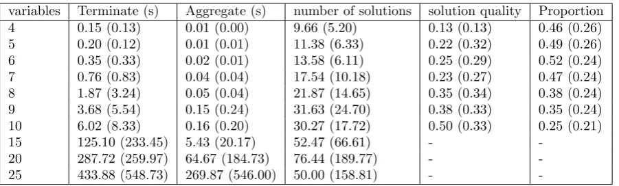
Table 4.1: Performance of SBDOsr. See text for description of metrics.
variables Terminate (s) Aggregate (s) number of solutions solution quality Proportion 4 0.15 (0.13) 0.01 (0.00) 9.66 (5.20) 0.13 (0.13) 0.46 (0.26) 5 0.20 (0.12) 0.01 (0.01) 11.38 (6.33) 0.22 (0.32) 0.49 (0.26) 6 0.35 (0.33) 0.02 (0.01) 13.58 (6.11) 0.25 (0.29) 0.52 (0.24) 7 0.76 (0.83) 0.04 (0.04) 17.54 (10.18) 0.23 (0.27) 0.47 (0.24) 8 1.87 (3.24) 0.05 (0.04) 21.87 (14.65) 0.35 (0.34) 0.38 (0.24) 9 3.68 (5.54) 0.15 (0.24) 31.63 (24.70) 0.38 (0.33) 0.35 (0.24) 10 6.02 (8.33) 0.16 (0.20) 30.27 (17.72) 0.50 (0.33) 0.25 (0.21)
15 125.10 (233.45) 5.43 (20.17) 52.47 (66.61) -
-20 287.72 (259.97) 64.67 (184.73) 76.44 (189.77) - -25 433.88 (548.73) 269.87 (546.00) 50.00 (158.81) -
-2. (Aggregate) Time to aggregate the partial solutions. 3. (number of solutions) Total number of solutions found.
4. (solution quality) The average of the minimum euclidean distance from the utility of each non-optimal solution to the utility of an optimal solution. Formally:
quality =
∑
n∈Nmin (f(n, o1), . . . , f(n, ox)) |N|
where f(x, y) is the euclidean distance between x and y, S is the set of the utilities of the solutions found by SBDOsr, O is the set of utilities of the optimal solutions andN =S/O.
5. (Proportion) The proportion of optimal solutions found. Formally:
proportion = |O∩S| |O|
Note that the set of optimal solutions must be known to compute metrics four and five. We used exhaustive search to find all the optimal solutions for problems with up to ten variables, it proved to be infeasable to solve bigger problems using exhaustive search.
Because each agent only has a local view of the problem a post-processing step is required to combine all the partial solutions into complete solutions. Whether this step is required depends on the problem being solved, decision support applications will require complete solutions, but some things like autonomous robots may be able to function using only local knowledge. It also depends on how many solutions are desired, for these experiments we extracted all pareto-optimal solutions found by SBDOsr. Because of this, we have presented the time required for the algorithm to terminate and the time to aggregate the partial solutions into global solutions separately.
The performance of SBDOsr is shown in Table 1. The number of constraints in the problem had very little effect on the performance, so we have not reported those results here. As expected, the number of variables in the problem has a large impact on the performance. Both the time required for the algorithm to terminate and the number of solutions found when the algorithm does terminate increases exponentially as the number of variables increases. Furthermore, the time required to aggregate all solutions is dependant on the number of solutions, so aggregation time also rises exponentially as the number of solutions increases.
The standard deviations show that the performance of SBDOsr is highly unstable, often the standard deviation is greater than the mean. This is due to the highly non-deterministic nature of the SBDOsr algorithm. The order in which agents preform actions introduces a search bias. This bias determines which solutions are found and how much effort is required to terminate.
points discovered on the actual pareto-front drops off as the number of variables increases, the solutions found remain close to the actual pareto-front.
In the process of solving these problems, SBDOsr generates a large number of nogoods. As our implementa-tion of SBDOsr only has relatively simple code for searching and checking nogoods, this represents a significant performance bottleneck and contributes to the time required for the larger problems.
5. Conclusion. We have presented a modification of SBDO to support problems with multiple objectives, or in general, any DCOP problem where there does not exist a total pre-order over the set of solutions. In order to represent these problems, we propose a new definition of a DCOP using an idempotent semiring to measure the cost/utility of a solution. The SBDO algorithm was then modified to use this new definition. To solve problems of this form, each agent maintains multiple candidate solutions simultaneously. The partial solutions maintained by each agent can then be combined into a set of complete solutions.
Empirical evaluation shows that the algorithm finds a good approximation of the pareto-frontier, however the post-processing step to combine each agent’s partial solutions into complete solutions requires significant computational effort, and is currently done centrally. While this is a weakness of this approach, in situations such as autonomous robot control where complete solutions are not required for the agents to act, such a weakness is acceptable.
REFERENCES
[1] U. Bertele and F. Brioschi,Nonserial Dynamic Programming, Academic Press, 1972.
[2] G. Billiau, C. F. Chang, and A. Ghose,SBDO: A New Robust Approach to Dynamic Distributed Constraint Optimisation,
in Principles and Practice of Multi-Agent Systems, 2010.
[3] S. Bistarelli, U. Montanari, and F. Rossi,Semiring-based constraint satisfaction and optimization, J. ACM, 44 (1997),
pp. 201–236.
[4] K. M. Chandy and L. Lamport,Distributed Snapshots: Determining global states of distributed systems, ACM Transactions
on Computer Systems, 3 (1985), pp. 63–75.
[5] R. Dechter,Bucket elimination: A unifying framework for reasoning, in Articial Intelligence, vol. 113, 1999, pp. 41–85.
[6] R. Dechter and I. Rish,Mini-buckets: A general scheme for bounded inference, in Journal of the ACM, vol. 50, Mar 2003,
pp. 107–153.
[7] F. M. D. Fave, R. Stranders, A. Rogers, and N. R. Jennings,Bounded Decentralised Coordination over Multiple
Objec-tives, in AAMAS, 2011, pp. 371–378.
[8] T. Grinshpoun, A. Grubshtein, R. Zivan, A. Netzer, and A. Meisels,Asymmetric distributed constraint optimization
problems, J. Artif. Intell. Res. (JAIR), 47 (2013), pp. 613–647.
[9] P. Harvey,Solving Very Large Distributed Constraint Satisfaction Problems, PhD thesis, University of Wollongong, 2010.
[10] P. Harvey, C. F. Chang, and A. Ghose, Support-based distributed search: a new approach for multiagent constraint
processing, in AAMAS ’06, ACM, 2006, pp. 377–383.
[11] J. Larrosa,On arc and node consistency in weighted CSP, in proc. of AAAI’02, 2002, pp. 48–53.
[12] P. J. Modi, W.-M. Shen, M. Tambe, and M. Yokoo,ADOPT: asynchronous distributed constraint optimization with quality
guarantees, Artificial Intelligence, 161 (2005), pp. 149–180.
[13] J. P. Pearce and M. Tambe,Quality Guarantees on k-Optimal Solutions for Distributed Constraint Optimization Problems,
in IJCAI, M. M. Veloso, ed., 2007, pp. 1446–1451.
[14] A. Petcu,A class of algorithms for Distributed Constraint Optimistation, PhD thesis, ´Ecole Polytechnique F´ed´erale de
Lausanne, Oct 2007.
[15] A. Petcu and B. Faltings,DPOP: A Scalable Method for Multiagent Constraint Optimization, in IJCAI 05, Aug 2005,
pp. 266–271.
[16] E. Rollon,Multi-objective Optimization in Graphical Models, PhD thesis, Universitat Polit`ecnica de Catalunya, 2008.
[17] A. Rosenfeld,An Introduction to Algebraic Structures, Holden-Day, 1968.
[18] F. Rossi, P. van Beek, and T. Walsh, eds.,Handbook of Constraint Programming, Elsevier, 2006.
[19] T. Schiex and G. Verfaillie,Nogood Recording for Static and Dynamic Constraint Satisfaction Problem, International
Journal of Artifical Intelligence Tools, 3 (1994), pp. 187–207.
[20] M. C. Silaghi and M. Yokoo,Nogood based asynchronous distributed optimization (ADOPT-ng), in AAMAS ’06, ACM,
2006, pp. 1389–1396.