Multigrid Backprojection Super–Resolution and Deep Filter Visualization

(1)

The Thirty-Third AAAI Conference on Artificial Intelligence (AAAI-19)

Multigrid Backprojection

Super–Resolution and Deep Filter Visualization

Pablo Navarrete Michelini, Hanwen Liu, Dan Zhu

BOE Technology Group Inc., Ltd.

Beijing, China

Abstract

We introduce a novel deep–learning architecture for image upscaling by large factors (e.g.4×,8×) based on examples of pristine high–resolution images. Our target is to reconstruct high–resolution images from their downscale versions. The proposed system performs a multi–level progressive upscal-ing, starting from small factors (2×) and updating for higher factors (4×and8×). The system is recursive as it repeats the same procedure at each level. It is also residual since we use the network to update the outputs of a classic upscaler. The network residuals are improved by Iterative Back–Projections (IBP) computed in the features of a convolutional network. To work in multiple levels we extend the standard back– projection algorithm using a recursion analogous to Multi– Grid algorithms commonly used as solvers of large systems of linear equations. We finally show how the network can be interpreted as a standard upsampling–and–filter upscaler with a space–variant filter that adapts to the geometry. This approach allows us to visualize how the network learns to up-scale. Finally, our system reaches state of the art quality for models with relatively few number of parameters.

Introduction

In this work, we focus on the problem of image upscaling using convolutional networks. Upscaling signals by integer factors (e.g.2×,3×) is understood in classical interpolation theory as two sequential processes: upsample (insert zeros) and filter (Proakis and Manolakis 2007; Mallat 1998). Stan-dard upscaler algorithms, such as Bicubic or Lanczos, find high–resolution images with a narrow frequency content by using fixed low–pass filters. Similar to the classic upscaling model, the image acquisition can be modeled as low-pass filtering a high resolution image and then downsample the result (drop pixels). In test scenarios often used in bench-marks we actually know the exact downscaling model, e.g. Bicubic downscaler. The Iterative Back–Projection (IBP) al-gorithm (Irani and Peleg 1991) is often used to enforce the downscaling model for a given upscaler and get closer to the original image.

More advanced upscalers follow geometric principles to improve image quality. For example,edge–directed interpo-lationuses adaptive filters to improve edge smoothness (Al-gazi, Ford, and Potharlanka 1991; Li and Orchard 2001), or

bandletmethods use both adaptive upsampling and filtering (Mallat and Peyre 2007). More recently, machine learning has been able to use examples pairs of high and low reso-lution images to estimate the parameters of upscaling sys-tems (Park, Park, and Kang 2003). In some cases, the opti-mization approach of machine learning hides the connection with classical interpolation theory, e.g. sparse representation with dictionaries (Yang et al. 2008; 2010). In other cases, the adaptive filter approach is explicit, e.g. RAISR (Romano, Isidoro, and Milanfar 2016).

Upscaling using convolutional networks started with SR-CNN (Dong et al. 2014a; 2015) motivated by the suc-cess of deep–learning methods in image classification tasks (LeCun, Bengio, and Hinton 2015) and establishing a strong connection with sparse coding methods (Yang et al. 2008; 2010). SRCNN has later been improved, most notably by EDSR (Lim et al. 2017) and DBPN (Haris, Shakhnarovich, and Ukita 2018). Our system shares the con-volutional network approach but follows a different motiva-tion. Namely, we aim to reveal a strong connection between convolutional–networks and classical image upscaling. By doing so, we can recover the classic interpretation of upsam-pling and filter and visualize what is the network doing pixel by pixel. Thus, we aim to prove that convolutional networks are a natural and convenient choice for Super–Resolution (SR) tasks.

Our main contributions are:

• We extend the IBP algorithm to amulti–level IBP.

• We prove that our algorithmworks as well as classic IBP, based on an unrealistic model.

• We introduce a new network architecture that over-comes the unrealistic model and allows us to learn both upscaling and downscaling.

• We introduce a novel algorithm to analyze the linear components of the network.

• We show how tointerpret the networkas a standard up-scaler with adaptive filters.

Related Work

(2)

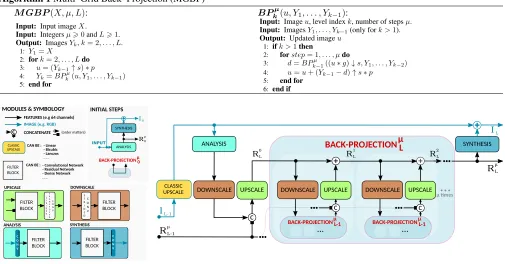
Algorithm 1Multi–Grid Back–Projection (MGBP)

M GBP(X, µ, L): BP_kµ(u, Y1, . . . , Yk−1):

Input: Input imageX.

Input: Integersµ>0andL>1.

Output: ImagesYk,k= 2, . . . , L.

1:Y1=X

2:fork= 2, . . . , Ldo

3: u= (Yk−1↑s)∗p

4: Yk=BP µ

k(u, Y1, . . . , Yk−1)

5:end for

Input:Imageu, level indexk, number of stepsµ.

Input:ImagesY1, . . . , Yk−1(only fork >1).

Output:Updated imageu

1: ifk >1then

2: forstep= 1, . . . , µdo

3: d=BP_kµ−1((u∗g)↓s, Y1, . . . , Yk−2)

4: u=u+ (Yk−1−d)↑s∗p

5: end for

6: end if

+

...

SYNTHESIS + RL-1 μ IL-1 RL 0 RL 1 RL 2 ... INITIAL STEPS INPUT + I 0 R0 μ c c + ... FILTER BLOCK S T R I D E D C O N V DOWNSCALE ANALYSIS FILTER BLOCK C O N V UPSCALE FILTER BLOCK S T R I D E D C O N V T R A N S P O S E D FILTER BLOCK

CAN BE :

c

BACK-PROJECTIONμ_L

BACK-PROJECTIONμ_L-1 BACK-PROJECTIONμ_L-1

BACK-PROJECTIONμ₀

UPSCALE DOWNSCALE

CLASSIC UPSCALE

ANALYSIS FEATURES (e.g 64 channels)

IMAGE (e.g. RGB)

RL μ IL SYNTHESIS ANALYSIS UPSCALE

DOWNSCALE DOWNSCALE UPSCALE

CLASSIC UPSCALE

CAN BE : - Linear - Bicubic - Lanczos . . .

- Convolu�onal Network - Residual Network - Dense Network . . . SYNTHESIS FILTER BLOCK C O N V CONCATENATE

MODULES & SYMBOLOGY

c (order ma�ers)

μ�mes

Figure 1: Multigrid Back–Projection (MGBP) system architecture. Lines indicate a number of image channels moving to different processing blocks, and line colors indicate the number of channels. Blue represents3channels for RGB images, and black represents the number of features managed by convolutional networks (latent space). At levelk the current upscaled image is indicated asIk and residuals in latent space are indicated asRk. We useAnalysisandSynthesismodules to transfer

images into latent space and vice versa. InInitial Stepswe obtain the first pair of output imageI0and residualR0, from the

input image. Then, the main diagram shows how to obtain the pairILandRLfrom the previous pairIL−1andRL−1. In red

we show the Back–Projection module, which repeats mu back–projection steps recursively.

• Multi–Scale Laplacian Super–Resolution (MSLapSR) (Lai et al. 2017b): Our system is inspired by MSLapSR to progressively upscale images using a classic upscaler and network updates, before back–projections that improve network updates in lower–resolutions. Both MSLapSR and our systems includeanalysisandsynthesisnetworks to convert images to latent space and vice versa. Both systems share parameters at each scale. Our system dif-fers mostly in the use of back–projections, that cannot be removed to recover MSLapSR because of the particular structure of ourupscalernetwork module.

• Deep Back–Projection Network (DBPN) (Haris, Shakhnarovich, and Ukita 2018): To the extent of our knowledge, this is the first reference to use IBP in a network architecture. It is also the state–of–art in terms of image quality, surpassing EDSR(Lim et al. 2017), former winner of NTIRE 2017 SR Challenge (Timofte et al. ). Their approach to use back–projections is different than ours because: first, their system is not multi–scale; and second, they iterate down and up projections. Our multi– scale architecture requires less number of parameters, because we reuse modules at every scale, and it is more flexible, because many upscaling factors can be achieved with the same modules. Also, our system is built upon an algorithm that is proven to converge, whereas, to the

extent of our knowledge, mixing up and down projections has no convergence guarantees.

Our contributions add to the following lines of research:

(3)

INPUT 2×

8×

No Recursion (μ=0) W-Cycle (μ=2)

c

4×

INPUT 2×

8×

V-Cycle (μ=1)

4× INPUT 2× 8× 4× c SYNTHESIS

ANALYSIS UPSCALE DOWNSCALE CLASSIC UPSCALE CONCATENATE

SC A LE c c c c c c c c c

c c c c

c

c c c c

c c

c c c c

c c c c c c c c + + + + + + + + + + + + + + + + + + + + + + + + + + + + + + + + + + + PROCESSING + + + + + c c

Figure 2: Multi–Grid Back–Projection (MGBP) recursion unfold from Figure 1 for different values ofµ, and three levels to output2×,4×and8×upscale images. Our system uses a recursion analogous to the Full–Multigrid algorithm to solve linear equations and leads to the well known workflows V–cycle forµ= 1and W–cycles forµ= 2(Trottenberg and Schuller 2001). After every upscaling step, the MGBP recursion sends the output down to every lower–resolution level in order to validate the downscaling model. The corrections are back-projected to higher resolutions.

All these approaches differ to ours in the fact that our recursion iterates back and forth between different reso-lutions. In numerical methods, such iterations have been used by two types of linear equation solvers: multi–

grid and domain decomposition methods (Trottenberg

and Schuller 2001; Widlund and Toselli 2004). We fol-low the multi–grid approach, that can use inductive ar-guments to study convergence, and leads to specific pro-cessing workflows to move intermediate results between scales (see for example the W–cycle in Figure 2). Systems like MS–DenseNet (Huang et al. 2017a) also move back and forth between scales with more simplified workflows but they were not designed based on classical methods. The connection to classical methods gives us a justifica-tion of these workflows that, otherwise, would be arbi-trary (e.g. why traversing scales with V or W workflows in Figure 2)? which workflow is better?) We will show, for example, how different numbers of back–projections (related to depth) make outputs sharper, same as in IBP. Our main contribution here is to devise a new algorithm that introduces the multi–grid recursion into IBP. It is a different algorithm than IBP, that we prove to converge at the same rate, and then extend to a network architecture. Finally, this effort pays back since our recursion works well in experiments, with no other method reaching the same quality with the same number of parameters.

• Network Visualization: A major direction of research in deep–learning is how to visualize the inner processing of a given architecture (Zhang and Zhu 2018). Among these, a line of research onfeature visualizationstudies what does a network detect (Olah, Mordvintsev, and Schubert 2017). Feature visualization can give example inputs that cause desired behaviors, separating image areas causing behav-ior from those that only relate to the causes. Another line of work onattributionstudies how does a network assem-bles these individual pieces to arrive at later decisions, or why these decisions were made (Olah et al. 2018). Our vi-sualization technique belongs to the latter because we can show how the input pixels are assembled into a particu-lar output pixel. We target the SR problem where there is extensive knowledge of non–adaptive filters (e.g. lin-ear, bicubic, etc.) built upon signal processing theory. The

ReLU ReLU G= _/ G zeros zeros + -· For each ac�va�on compute pixelwise gain:

- Replace ac�va�on with ﬁxed mask

X(i, j)= 1

GENERATES IMPULSE RESPONSE AT

(i, j) ReLU (si, sj) ORIGINAL SYSTEM EFFECTIVE RESIDU AL EFFECTIVE FILTER

Figure 3: Activation freezing procedure to convert a network into a linear system. We can perform impulse response anal-ysis to study the overall filter effect at each pixel location.

+

=

↑

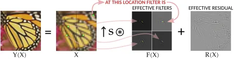
s

_*

AT THIS LOCATION FILTER IS

EFFECTIVE FILTERS EFFECTIVE RESIDUAL

Y(X) X F(X) R(X)

Figure 4: Interpretation of the upscaling network as a stan-dard upscaler with adaptive filters.

main novelty of our technique is that it provides an al-ternative system to replace the network for a given input. The new system generates the exact same outputs of the network from the same input images but, unlike the net-work, it is fully interpretable in the sense that we know what to expect from its parameters.

Multigrid Backprojections

A simple and common model for the downscaling process is

X = (Y ∗g)↓s , (1)

where Y is the high–resolution source, X is the low– resolution result,g is a blurring kernel and↓ sis a down-sampling by factors.

(4)

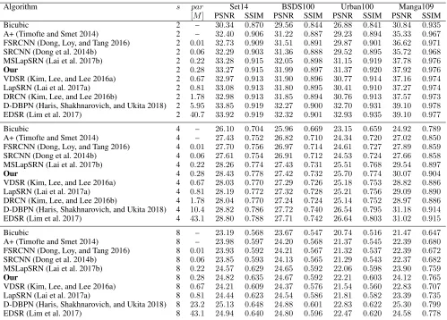
Table 1: Quantitative evaluation of different SR methods. Methods are ordered by increasing number of parameters.

Algorithm s par Set14 BSDS100 Urban100 Manga109

[M] PSNR SSIM PSNR SSIM PSNR SSIM PSNR SSIM

Bicubic 2 – 30.34 0.870 29.56 0.844 26.88 0.841 30.84 0.935

A+ (Timofte and Smet 2014) 2 – 32.40 0.906 31.22 0.887 29.23 0.894 35.33 0.967

FSRCNN (Dong, Loy, and Tang 2016) 2 0.01 32.73 0.909 31.51 0.891 29.87 0.901 36.62 0.971

SRCNN (Dong et al. 2014b) 2 0.06 32.29 0.903 31.36 0.888 29.52 0.895 35.72 0.968

MSLapSRN (Lai et al. 2017b) 2 0.22 33.28 0.915 32.05 0.898 31.15 0.919 37.78 0.976

Our 2 0.28 33.27 0.915 31.99 0.897 31.37 0.920 37.92 0.976

VDSR (Kim, Lee, and Lee 2016a) 2 0.67 32.97 0.913 31.90 0.896 30.77 0.914 37.16 0.974

LapSRN (Lai et al. 2017a) 2 0.81 33.08 0.913 31.80 0.895 30.41 0.910 37.27 0.974

DRCN (Kim, Lee, and Lee 2016b) 2 1.78 32.98 0.913 31.85 0.894 30.76 0.913 37.57 0.973

D-DBPN (Haris, Shakhnarovich, and Ukita 2018) 2 5.95 33.85 0.919 32.27 0.900 32.70 0.931 39.10 0.978

EDSR (Lim et al. 2017) 2 40.7 33.92 0.919 32.32 0.901 32.93 0.935 39.10 0.977

Bicubic 4 – 26.10 0.704 25.96 0.669 23.15 0.659 24.92 0.789

SRCNN (Dong et al. 2014b) 4 0.06 27.61 0.754 26.91 0.712 24.53 0.724 27.66 0.858

Our 4 0.28 28.43 0.778 27.42 0.732 25.70 0.774 30.07 0.904

LapSRN (Lai et al. 2017a) 4 0.81 28.19 0.772 27.32 0.728 25.21 0.756 29.09 0.890

DRCN (Kim, Lee, and Lee 2016b) 4 1.78 28.04 0.770 27.24 0.724 25.14 0.752 28.97 0.886

EDSR (Lim et al. 2017) 4 43.1 28.80 0.788 27.71 0.742 26.64 0.803 31.02 0.915

Bicubic 8 – 23.19 0.568 23.67 0.547 20.74 0.516 21.47 0.647

SRCNN (Dong et al. 2014b) 8 0.06 23.85 0.593 24.13 0.565 21.29 0.543 22.37 0.682

Our 8 0.28 24.82 0.635 24.67 0.592 22.21 0.603 24.12 0.765

LapSRN (Lai et al. 2017a) 8 0.81 24.44 0.623 24.54 0.586 21.81 0.582 23.39 0.735

EDSR (Lim et al. 2017) 8 43.1 24.94 0.640 24.80 0.596 22.47 0.620 24.58 0.778

Peleg 1991). Given model (1) and an upscaled imageY, the IBP algorithm iterates:

e(Yk) = X−(Yk∗g)↓s (2)

Yk+1 = Yk+e(Yk)↑s∗p . (3)

Here,e(Yk)is the mismatch error at low–resolution,gandp

are blurring and upscaling filters, respectively. The iteration is proven to converge, to enforce model (1) at exponential rate (Irani and Peleg 1991).

To make IBP work for multiple scales we change model (1) to:

X= (· · ·((Y ∗g)↓s∗g)↓s· · · ∗g)↓s

| {z }

Ltimes

. (4)

This is not a common downscaling procedure in practice and might be the reason why multi–scale IBP has not been con-sidered yet. We will later replace the downscaling by a net-work so that model (4) becomes flexible and is able to learn a direct downscaling or even more complex models.

Upscaling images with IBP is a two–step process: first, upscale an image; and second, improve it with IBP. This is reminiscent of the way a Full–Multigrid algorithm solves linear equations (Trottenberg and Schuller 2001). This is:

first, find an approximate solution; and second, improve it by solving an equation for the approximation error. Both IBP and Multigrid iterate between different scales, but IBP only uses two levels whereas Multigrid recursively move to coarser grids. We use the same strategy as in Multigrid to define a so–calledMulti–Grid Back–Projectionalgorithm as shown in Algorithm 1. Here, back–projections recursively return to the lowest–resolution enforcing the downscaling model at each scale.

ForL= 2the MGBP algorithm and model (4) are equiva-lent to the original IBP (Irani and Peleg 1991) and model (1), and thus converges at exponential rate. In section A of the supplementary material we prove convergence forL > 2. Basically, the algorithm inherits the exponential rate con-vergence from the two–level case through the recursion in Algorithm 1.

Network Architecture

We convert the Multi–Grid Back–Projection algorithm into a network structure as follows:

(5)

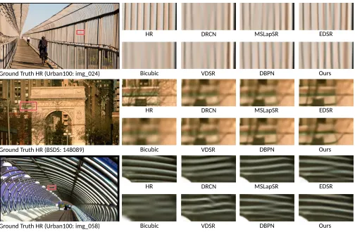
HR DRCN MSLapSR EDSR

Bicubic VDSR DBPN Ours

Ground Truth HR (Urban100: img_024)

Ground Truth HR (BSDS: 148089)

Figure 5: Perceptual evaluation of different SR methods for4×upscaling.

HR MSLapSR EDSR

Bicubic DBPN Ours

Figure 6: Perceptual evaluation of different SR methods for8×upscaling.

• Step 2: Transfer the upscale imageIinto latent space us-ing a network Analysis(I).

• Step 3: In latent space we apply the recurrence in Algo-rithm 1 by changing:

– (u∗g)↓sinto a network Downscale(u).

– (Yk−1−d)↑s∗pinto a network Upscale([Yk−1, d]).

Where[Yk−1, d]is the concatenation of features and

re-places the subtraction. Thus, theUpscalernetwork re-ceives double the number of features in the input com-pared to the output.

Figure 1 shows the definition of our network architecture.

The unfolded recursion is shown in Figure 2 for three differ-ent values ofµ.

Deep Filter Visualization

Deep Learning architectures are highly non–linear, although much of their internal structure is linear (e.g. convolutions). We want to study the overall effect of the linear structure of the network. The general procedure is shown in Figure 3 and is as follows:

(6)

↑

*

8

F

SP

A

CE

FRE

QUEN

CY

R

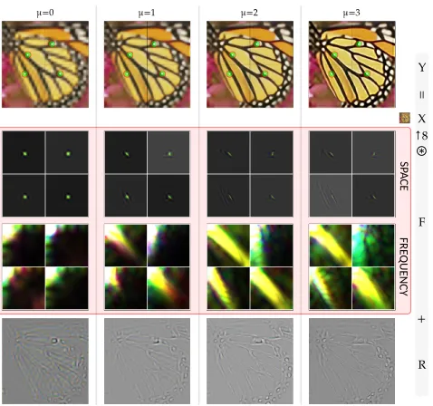
μ=0 μ=1 μ=2 μ=3

Y

=

+

X

Figure 7: Output images for 8× upscaling using different numbers of back–projections µ. The network was trained withµ = 2fixed. The effective filters are shown together with their frequency response (FFT).

• At each non-linear layer we record how much did the in-put change (layer gain).

• We replace (freeze) all non–linearities by the fix gain pre-viously recorded. The overall system becomes linear, such thatY =F X+R.

• We obtain theeffective residualRwith an inputX= 0in the activation frozen system.

• We obtain theeffective filterfor a particular input pixel by using aδinput centered at the pixel location, and subtract the residualRfrom the output. In linear system terminol-ogy we are computing theimpulse responseof the system (Proakis and Manolakis 2007).

We can obtain explicit formulas forF andRif we con-sider a model of convolutional network as a sequence of lin-ear and nonlinlin-ear layers:

zn=Wnxn−1+bn and xn=σ(zn) , (5)

wherexnandznare vectorized features at layern, after and

before activations, respectively. The parameters of the net-work are the biasesbnand the sparse matricesWn

represent-ing the convolutional operators (also applies for strided and transposed convolutions). For a given input imageX, the in-put of the model isx0 = vec(X)(vectorized image). The

output imageY, afternconvolutional layers, is vec−1(xn).

Definition 1 (Activation Gain) The gain of an activation functionσis given byG(x)[i] =σ(x[i])/x[i]and equal to1

ifx[i] = 0.

Theorem 1 (Activation Freeze) LetWˆn =G(zn)Wnand

(a)4×results on Set14

(b)8×results on Set14

Figure 8: Quality vs Complexity of different SR methods.

ˆ

bn=G(zn)bn. Let

Q0=I , Qi= n

Y

k=n−i+1 ˆ

Wk, fori= 1, . . . , n . (6)

The output of the convolutional network is given byxn =

F x0+R, whereF = Qn is theeffective filterandR =

Q∗ˆb=Pn

k=0Qkˆbn−kis theeffective residual.

The proof of the theorem is a direct consequence ofσ(x) =

G(x)xand expansion of (5). Although this theorem only ap-plies to sequential networks, it helps to show that the overall effective filter depends on all convolutional filters as well as biases (only through activations). Similarly, the effective residual depends on both convolutional filters and biases (both explicitly and through activations).

For the sake of simplicity, here we use our visualization technique from input to outputs of the network. Neverthe-less, we note that we could start at any layer and stop at any posterior layer to study attributions within the network.

Experiments

We use onesingle configurationto test our system for2×,

4×, and8×upscaling. We configure theAnalysis,Synthesis,

UpscaleandDownscalemodules in Figure 1 using4–layer

(7)

EFFECTIVE FILTERS EFFECTIVE RESIDUAL OUTPUT IMAGE & PROBES

4×

8×

Figure 9: Effective filters and residual for4×and8×upscaler. . Filters are not only directional but follow several features around a pixels. Residuals are in general small and thus most of the work is done by the filters.

For training the system we fix the number of back– projections toµ = 2(W–cycle according to Figure 2). We train the system for 8×upscaler with the multi–scale loss function introduced in (Lai et al. 2017b):

L(Y, X;θ) = X L=1,2,3

L

X

k=1

E||YkL−Xk||1

. (7)

We train our system with Adam optimizer and a learning rate initialized as10−3_{and square root decay. We use}₁₂₈_×₁₂₈

patches (pieces of images) with batch size16. The patches were sampled randomly from datasets DIV2K and Flickr2K, containing photographs of general natural scenes.

Comparisons

In Table 1 we compare PSNR and SSIM values for differ-ent methods. The two evaluation metrics measure the dif-ference between an upscaler output and the original high-resolution image. Higher values are better in both cases. Roughly speaking, PSNR (range0to∞) is a log–scale ver-sion of mean–square–error and SSIM (range 0 to 1) uses image statistics to better correlate with human perception.

Full expressions are as follows:

P SN R(X, Y) = 10·log₁₀

2552

M SE

, (8)

SSIM(X, Y) = (2µXµY +c1)(2σXY +c2) (µ2

X+µ

2

Y +c1)(σ2X+σ

2

Y +c2)

, (9)

whereM SE = mean((X −Y)2₎_{is the mean square}

er-ror ofX andY;µX andµY are the averages ofX andY,

respectively;σ2

X andσY2 are the variances ofX andY,

re-spectively;σXY is the covariance of X and Y;c1 = 6.5025

andc2= 58.5225.

Our method is outperformed only by EDSR and DBPN, that use20to more than100times the number of parame-ters of our system. Among systems with less than2million parameters, our system obtains better results, only matched by MSLapSR for2×upscaling.

In Figure 8 we better visualize the difference in complex-ity between different systems. It is apparent from these re-sults that the size of the system matters to improve PSNR values, with EDSR and DBPN far from other methods, but the cost can be overwhelming in performance. Our system clearly improves the state of the art for systems with less than two million parameters, with better quality and signifi-cantly less parameters.

(8)

out-puts look sharper and show consistent geometry. But often we find patches with aliasing, such as parallel lines, where the geometry becomes chaotic and perceptual quality be-haves randomly. In such cases our system can take advan-tage compared to most of other systems.

Analysis

Figure 9 shows two examples of effective filters and residu-als according to our novel visualization method. The shapes of filters following edges are reminiscent of the research on directional filter upscalers (Algazi, Ford, and Potharlanka 1991; Li and Orchard 2001). In general, we observe that filters are highly adaptive. They become symmetric and narrow in flat areas (like Linear or Bicubic upscalers), direc-tional close to sharp lines, and increase in size close to com-plex features. For example, in the4×upscale of Figure 9 a red box shows an area with the eye of a baboon and the wrin-kles around its eye. In the filter we can observe the shape of the eye and waves following the wrinkles. As expected, for8×upscaler the receptive field increases since the filters look bigger. We remind that we are using the same number of parameters, but passing through more layers. In the green box in 9 we highlight the face and hand of a woman. The filter at the tip of the nose follows the face features, and the filter at the hand captures features from all the edges around. Figure 7 shows the effect of the depth on the effective fil-ters and residuals. Here, training has tuned the network to work best withµ= 2back–projections. Forµ >2the out-put image looks oversharp, and too soft forµ < 2. Accord-ingly, filters are larger and extract more high–frequencies forµ >2and become smaller and low-pass forµ <2. The same effect is observed with classic IBP (Irani and Peleg 1991), showing the effective design of our network architec-ture.

We observe that residuals are in general small and help fixing textures and small details. This is an indication that filters are doing most of the work for upscaling. We remind that, after freezing activations, the residual is a fixed compo-nent of the output that does not change with the input. Thus, residuals are very limited to estimate local details in the out-put as they depend only on activations for this purpose.

On the other hand, filters contain relations between neigh-boring pixels and we argue that because of this they are bet-ter to generalize. Effective filbet-ters also show all the details regarding the receptive field of the network. The receptive field is adaptive as the network does not use neighboring pixels if it does not need to (e.g. flat areas) and extend to large areas when the network is deep (e.g.8×upscaler) and local details are complex.

Finally, we remind that this analysis is precise. The net-work can be replaced by these adaptive filters plus residuals and it would give the exact same output. The strong depen-dency of filters and residuals on the input image shows all the non–linearities of the network. It is remarkable that con-volutional networks can achieve the level of adaptivity re-vealed by these visualization experiments and it further jus-tifies their success in super–resolution tasks.

Conclusions

We introduced a new architecture for single image super– resolution that reaches state of the art for methods with less that 2 million parameters and a new technique to analyze the network. The analysis shows how the network learns to upscale by capturing complex relationships between pixels.

References

Algazi, V. R.; Ford, G. E.; and Potharlanka, R. 1991. Di-rectional interpolation of images based on visual properties and rank order filtering. InProc. IEEE Int. Conf. Acoustics, Speech, Signal Processing, volume 4, 3005–3008. Toronto, ON: IEEE Signal Processing Society.

Diamond, S.; Sitzmann, V.; Heide, F.; and Wetzstein, G. 2017. Unrolled optimization with deep priors. CoRR abs/1705.08041.

Dong, C.; Loy, C.; He, K.; and Tang, X. 2014a. Learning a deep convolutional network for image super–resolution. In et al., D. F., ed., Proceedings of European Conference on

Computer Vision (ECCV), volume 8692 ofLecture Notes in

Computer Science, 184–199. Zurich: Springer.

Dong, C.; Loy, C. C.; He, K.; and Tang, X. 2014b. Learning a deep convolutional network for image super–resolution. In in Proceedings of European Conference on Computer Vision (ECCV).

Dong, C.; Loy, C.; He, K.; and Tang, X. 2015. Image super–resolution using deep convolutional networks. IEEE Transactions on Pattern Analysis and Machine Intelligence 38(2):295–307.

Dong, C.; Loy, C. C.; and Tang, X. 2016. Accelerating the super–resolution convolutional neural network. In in Proceedings of European Conference on Computer Vision (ECCV).

Gong, D.; Zhang, Z.; Shi, Q.; van den Hengel, A.; Shen, C.; and Zhang, Y. 2018. Learning an optimizer for image deconvolution. CoRRabs/1804.03368.

Haris, M.; Shakhnarovich, G.; and Ukita, N. 2018. Deep back–projection networks for super–resolution. In IEEE Conference on Computer Vision and Pattern Recognition (CVPR).

Huang, G.; Chen, D.; Li, T.; Wu, F.; van der Maaten, L.; and Weinberger, K. Q. 2017a. Multi-scale dense convolutional networks for efficient prediction. CoRRabs/1703.09844. Huang, G.; Liu, Z.; van der Maaten, L.; and Weinberger, K. Q. 2017b. Densely connected convolutional networks.

InProceedings of the IEEE Conference on Computer Vision

and Pattern Recognition.

Irani, M., and Peleg, S. 1991. Improving resolution by im-age registration. CVGIP: Graph. Models Image Process. 53(3):231–239.

Kim, J.; Lee, J. K.; and Lee, K. M. 2016a. Accurate image super–resolution using very deep convolutional networks.

In The IEEE Conference on Computer Vision and Pattern

Recognition (CVPR Oral).

(9)

IEEE Conference on Computer Vision and Pattern Recogni-tion (CVPR Oral).

Kokkinos, F., and Lefkimmiatis, S. 2018. Deep image demo-saicking using a cascade of convolutional residual denoising networks. CoRRabs/1803.05215.

Kruse, J.; Rother, C.; and Schmidt, U. 2017. Learning to push the limits of efficient fft-based image deconvolution.

InThe IEEE International Conference on Computer Vision

(ICCV).

Lai, W.-S.; Huang, J.-B.; Ahuja, N.; and Yang, M.-H. 2017a. Deep laplacian pyramid networks for fast and accurate super–resolution. InIEEE Conference on Computer Vision and Pattern Recognition.

Lai, W.-S.; Huang, J.-B.; Ahuja, N.; and Yang, M.-H. 2017b. Fast and accurate image super–resolution with deep lapla-cian pyramid networks. arXiv:1710.01992.

LeCun, Y.; Bengio, Y.; and Hinton, G. 2015. Deep learning.

Nature521(7553):436–444.

Li, X., and Orchard, M. T. 2001. New edge–directed interpolation. IEEE Transactions on Image Processing 10(10):1521–1527.

Lim, B.; Son, S.; Kim, H.; Nah, S.; and Lee, K. M. 2017. Enhanced deep residual networks for single image super– resolution. In The IEEE Conference on Computer Vision

and Pattern Recognition (CVPR) Workshops.

Mallat, S., and Peyre, G. 2007. A review of bandlet methods for geometrical image representation.Numerical Algorithms 44(3):205–234.

Mallat, S. 1998.A Wavelet Tour of Signal Processing. Aca-demic Press.

Olah, C.; Satyanarayan, A.; Johnson, I.; Carter, S.; Schubert, L.; Ye, K.; and Mordvintsev, A. 2018. The building blocks of interpretability. Distill. https://distill.pub/2018/building-blocks.

Olah, C.; Mordvintsev, A.; and Schubert, L. 2017. Fea-ture visualization. Distill. https://distill.pub/2017/feature-visualization.

Park, S.; Park, M.; and Kang, M. 2003. Super–resolution image reconstruction: a technical overview.Signal

Process-ing Magazine, IEEE20(3):21–36.

Proakis, J., and Manolakis, D. 2007.Digital Signal Process-ing. Prentice Hall international editions. Pearson Prentice Hall.

Romano, Y.; Isidoro, J.; and Milanfar, P. 2016. RAISR: rapid and accurate image super resolution.CoRRabs/1606.01299. Timofte, R., and Smet, V. D. 2014. Gool, “a+: Adjusted anchored neighborhood regression for fast super–resolution. Inin Proc. Asian Conf. Comput. Vis. (ACCV.

Timofte, R.; Agustsson, E.; Van Gool, L.; Yang, M.-H.; Zhang, L.; et al. Ntire 2017 challenge on single image super-resolution: Methods and results. InThe IEEE Conference on Computer Vision and Pattern Recognition (CVPR) Work-shops.

Trottenberg, U., and Schuller, A. 2001.Multigrid. Orlando, FL, USA: Academic Press, Inc.

Widlund, O., and Toselli, A. 2004. Domain decomposition methods - algorithms and theory, volume 34. Springer. Yang, J.; Wright, J.; Huang, T.; and Ma, Y. 2008. Im-age super–resolution as sparse representation of raw imIm-age patches. InIEEE Conference on Computer Vision and Pat-tern Recognition.

Yang, J.; Wright, J.; Huang, T.; and Ma, Y. 2010. Image super–resolution via sparse representation. Image

Process-ing, IEEE Transactions on19(11):2861–2873.

Zhang, Q., and Zhu, S. 2018. Visual interpretability for deep learning: a survey. Frontiers of Information Technology and

Electronic Engineering19(1):27–39.