Learning Adaptive Random Features

The Thirty-Third AAAI Conference on Artificial Intelligence (AAAI-19)

Learning Adaptive Random Features

Yanjun Li,

Kai Zhang,

Jun Wang,

Sanjiv Kumar

3_{East China Normal University,}4_{Google Research} 1_{[email protected],}2_{[email protected],} 3_{[email protected],}4_{[email protected]}

Abstract

Random Fourier features are a powerful framework to ap-proximate shift invariant kernels with Monte Carlo integra-tion, which has drawn considerable interest in scaling up kernel-based learning, dimensionality reduction, and infor-mation retrieval. In the literature, many sampling schemes have been proposed to improve the approximation perfor-mance. However, an interesting theoretic and algorithmic challenge still remains, i.e.,how to optimize the design of ran-dom Fourier features to achieve good kernel approximation on any input data using a low spectral sampling rate?In this paper, we propose to compute more adaptive random Fourier features with optimized spectral samples (wj’s) and feature

weights (pj’s). The learning scheme not only significantly

re-duces the spectral sampling rate needed for accurate kernel approximation, but also allows joint optimization with any supervised learning framework. We establish generalization bounds using Rademacher complexity, and demonstrate ad-vantages over previous methods. Moreover, our experiments show that the empirical kernel approximation provides effec-tive regularization for supervised learning.

Introduction

Despite the immense popularity of kernel-based learning al-gorithms (Sch¨olkopf and Smola 2002), the expensive eval-uation of nonlinear kernels has prohibited their applica-tion to large datasets. Low-rank kernel approximaapplica-tion is a powerful tool in alleviating the memory and computa-tional cost of large kernel machines (Williams and Seeger 2001; Drineas and Mahoney 2005; Fowlkes et al. 2004; Halko, Martinsson, and Tropp 2011; Mahoney 2011; Ku-mar, Mohri, and Talwalkar 2012; Si, Hsieh, and Dhillon 2014). These methods adopt various sampling schemes on the rows/columns of the kernel matrix to obtain an efficient, low-rank decomposition, which in turn serves as a highly compact “empirical” kernel map that can reduce the cost of kernel machines from cubic to linear scale.

Random Fourier features, a highly innovative feature map pioneered by Rahimi and Recht (2008), has attracted sig-nificant interest, which will also be the focus of our work. Rather than decomposing the kernel matrix directly, the

∗

Contact author.

Copyright c2019, Association for the Advancement of Artificial Intelligence (www.aaai.org). All rights reserved.

method resorts to the Fourier transform of positive semi-definite and shift-invariant kernels and obtains explicit fea-ture maps using Monte Carlo approximation of the Fourier representation. The features can then be written as the cosine (or sine) of the inner product between the input data and ran-dom spectral samples drawn from a density specified by the characteristic function. For example, the characteristic func-tion for Gaussian kernel is still Gaussian, hence the spectral samples should follow a Gaussian distribution.

In recent years, there has been continuing effort in de-signing optimal sampling schemes in computing Fourier features for accurate approximation. Le et al. (2013) pro-posed Fastfood, a feature map that is faster to compute thanks to a combination of diagonal Gaussian matrices and the Hadamard transform. Yang et al. (2014) showed that integral approximation using low-discrepancy quasi-Monte Carlo (QMC) sequence has a faster convergence than ran-dom Monte Carlo samples, and achieves lower error espe-cially for high-dimensional data. Shen et al. (2017) pro-posed to apply moment matching on the spectral samples so that their empirical distribution is closer to the intended Gaussian. Besides shift-invariant kernels, approximate fea-ture maps have also been considered for other nonlinear ker-nels, such as additive kernels (Vedaldi and Zisserman 2012), and polynomial kernels using spherical sampling (Penning-ton, Felix, and Kumar 2015). Despite these recent advances, open challenges still exist. First, most of the existing works ignore the impact of the input data distribution on the de-sign of the feature map. Instead, the main dependency con-sidered is the relation between the kernel and its charac-teristic function. Second, better kernel approximation with random Fourier features may not always translate to bet-ter generalization performance. Despite reported improve-ments in regression/classification, it has been found that such improvements do not correlate well with the improve-ments in the quality of kernel features (Avron et al. 2016; Chang et al. 2017).

approximat-ing the kernel Fourier transform, and demonstrate that the optimal proposal density should be adaptive to the input dis-tribution. Based on these observations, we propose a novel method to learn adaptive Fourier features, in which the spec-tral samples and their corresponding feature weights are op-timized jointly through minimization of the empirical kernel approximation loss (EKAL). We also propose two approxi-mators of the EKAL, so that an efficient iterative algorithm can be designed, reducing the overall time/space complexity to scale linearly with input sample size and dimension.

We want to emphasize some fundamental differences be-tween our method and existing randomized algorithms. In those methods, a sampling probability is computed to se-lect useful matrix columns often involving costly operations in the input space (e.g. SVD for leverage scores (Mahoney 2011) or computing norms of all matrix columns (Kumar, Mohri, and Talwalkar 2012). In comparison, we do not re-sort to any sampling strategy but instead explicitly optimize the spectral basis and weights in theFourierspace; besides, our approach is significantly cheaper and the cost of obtain-ing the basis can be as low as sub-linear. Recently (Bach 2017) proposed to select spectral samples by computing a discrete probability distribution over a large number of ref-erence points. Note that their goal is functional tion in the RKHS, while ours is kernel matrix approxima-tion; besides, sampling in a high-dimensional space can be quite challenging, while optimizing the spectral basis based on explicit objective function can be computationally more tractable and more convenient.

We establish rigorous generalization bounds tailored to the minimizers of the EKAL approximators, using Rademacher average and McDiarmid’s inequality. Unlike the loss function in a typical statistical learning problem, EKAL contains a small set of pairwise kernel evaluations that are not all independent. We overcome this challenge by creating independent games in statistically dependent

rounds based onround-robin tournament scheduling. Our bounds can be easily translated to guarantees for supervised learning, using results that connect low-rank kernel approxi-mation and learning accuracy (Cortes, Mohri, and Talwalkar 2010). These theoretical findings are complemented by nu-merical experiments, which show the clear advantage of our learned Fourier features over previous ones in kernel ap-proximation. Indeed, our method is the first to fully exploit the input data to significantly improve the quality of Fourier features, bridging the gap between data-driven methods and fixed-basis methods. Besides effectively reducing the di-mension of the kernel map (i.e., spectral sampling rate) to achieve desired accuracy, our method can also be incorpo-rated in any supervised learning framework. In particular, we employ EKAL minimization as a regularization to build-ing linear prediction models with learned Fourier features, leading to improved generalization performance.

Our main contributions include: (1) Theoretical justifi-cation of learning data-driven Fourier features using im-portance sampling as an example. (2) Joint optimization of spectral samples and feature weights in minimizing two types of EKAL approximators; generalization error bound for both. (3) Hybrid loss with both unsupervised kernel

regu-larization and supervised prediction loss to improve the per-formance in classification/regression. (4) Extensive experi-mental results both in kernel approximation and in super-vised learning tasks.

Random Fourier Features

Monte Carlo Method with Uniform Weights

Given a shift-invariant kernel function k, we wish to con-struct a feature mapZ(x)whose pairwise inner-product ap-proximates the kernel byk(x1−x2)≈ hZ(x1),Z(x2)i. By

doing this, the kernel matrixKdefined on{x`}N`=1can then

be approximated by a low-rank decompositionZZ>, where Kst=k(xs−xt)and thes-th row ofZisZ(xs).

Rahimi and Recht (2008) pioneered the use of Fourier transform in solving this problem, by noting that any PSD shift invariant kernel k can be reconstructed using the Fourier basis sampled under the probability density defined by the characteristic function ofk,

k(x1−x2) =

Z

Rd

eiw>(x1−x2)_{p(w)dw. (1)}

The density p(w) is the Gaussian PDF N(0, σ−2I) for Gaussian kernelk(x1−x2) = exp(−kx1−x2k2/(2σ2)).

Suppose the feature map is defined as

Z(x) := √1

r

h

eiw>1x_{, e}iw >

2x_{, ..., e}iw >

rx

i

, (2)

where{wj}r

j=1 ared-dimensional spectral samples drawn

independently from p(w). It can then be observed that

hZ(x1),Z(x2)i= 1_rP

r j=1e

iw>_j(x1−x2)_{, which is an} unbi-ased estimator of the Fourier representation of the kernel1_, and such a Monte Carlo approximation will asymptotically converge to the true integral (1) (Rahimi and Recht 2008).

Importance Sampling with Non-Uniform Weights

The sampling probabilityp(w) in Monte Carlo method is the characteristic function of the kernel. For a given ker-nel,p(w)is fixed regardless of the distribution of the input samples. However, given the input samplesxi’s, we believe that its distributionP(x)should also have an impact on the sampling probabilityp(w). In particular, the optimalp(w)

should be adaptive toP(x)in terms of accurately approxi-mating kernel matrix defined onP(x), using as few spectral samples (wj’s) as possible.

In order to see this, we consider the use of importance sampling, which is widely used in Bayesian inference to re-duce the variance of approximations. Sincekis real, one can rewrite the real part of Fourier representation as

k(x1−x2) =

Z

Rd

cos(w>(x1−x2))

p(w)

q(w)q(w)dw.

1

Since the kernel is real, one can remove the imaginary parts of (1) and (2). The real Fourier representation and features are k(x1−x2) =

R

Rdcos w

>

(x1−x2)

p(w)dw and Z(x) :=

1

√

r

cos(w1>x), . . . ,cos(w>rx),sin(w>1x), . . . ,sin(w>rx)

Here,q(w)is an importance-weighted proposal density. If wj’s are drawn from the distributionq(w), then we can ap-proximate the above integral with Pr

j=1pjcos(wj>(x1−

x2)), where pj = p(wj)/(r · q(wj)) satisfies E[pj] =

1/r. The above finite sample estimate is the inner product

hZe(x1),Ze(x2)ibetween weighted Fourier features:2

e

Z(x) :=√

p1cos(w>1x), ..., √

prcos(wr>x),

√

p1sin(w1>x), ..., √

prsin(w>rx)

. (3)

The optimal importance distribution minimizes the fol-lowing expected error, which depends on input distribution:

min

q(w)Ex1,x2Ewj

hZe(x1),Ze(x2)i −k(x1−x2)

2

. (4)

For example, in the casex1−x2is drawn from a Gaussian

distribution, we can prove the following.

Claim 1. Ifk(x1−x2) = exp(−kx1−x2k2/(2σ2)), and

x1−x2follows a Gaussian distributionN(0, σ02I), then the

optimalq(w)satisfies

q(w)∝e−σ2kwk2+e−(σ2+2σ02)kwk2 1/2

.

Claim 1 shows that the optimalq(w)depends on the input distributionP(x)(particularly onσ0). It follows that, in the

finite sample estimate, the choice of samples wj’s should also be data-dependent. Meanwhile, the corresponding fea-ture weightingpj=p(wj)/(r·q(wj))appears non-uniform and should depend on the input data distribution as well.

In practice, the underlying input distributionP(x)is un-known, hence solving (4) for the optimal importance distri-butionq(w)is intractable. Therefore, instead of designing the optimalq(w), we propose to learnwj’s (spectral sam-ples) and pj’s (corresponding feature weights) directly by minimizing the finite-sample kernel approximation error.

Adaptive Fourier Features

Empirical Kernel Approximation Loss

In this section, we explain howwj’s andpj’s in weighted Fourier features (3) can be learned efficiently from data. Suppose the input datax` belong to a compact setX. To simplify the notation, we define functionf :X − X →R, parametrized by{wj, pj}rj=1:

f(x1−x2) :=

r X

j=1

pjcos w>j(x1−x2).

The goal for kernel approximation is to learn the optimal wj ∈ W (1 ≤ j ≤ r) and p∈ ∆r−1 _{that minimizes the}

mean squared errorEx1,x2[(k(x1−x2)−f(x1−x2))

2_{]. If}

we restrict our attention to approximating the kernel matrix on a dataset{x`}N

`=1, the loss function is the mean squared

error over the empirical distribution over the dataset:

L(f) := 1 N2

N X

s=1

N X

t=1

(f(xs−xt)−k(xs−xt))2.

2

Uniformly weighted Fourier featuresZ(x)is a special case of

e

Z(x):q(w) =p(w)and hencepj= 1/r.

In this objective, we intend to optimize both wj’s and their weightspj’s. Such an optimization will adapt the re-sulting Fourier features to the input data, hence making them more likely to obtain desired approximation accuracy with minimal sampling rate in the spectral domain.

Evaluating k(xs−xt)over the whole sample is expen-sive and unnecessary. An important contribution of our work is to approximately evaluate the loss functionL(f)using a small numbernoflandmarkdata points (n N), similar to the idea of sketching for regression (Avron, Sindhwani, and Woodruff 2013; Woodruff and others 2014). We use the following two strategies to choose landmark points and com-pute empirical kernel approximation loss (EKAL):

Random sampling:We randomly samplenpoints from the dataset with equal probability without replacement, i.e., choose{x`<sub>1</sub>, . . . ,x`_n} ⊂ {x1, . . . ,xN}, and compute

Ls(f) := 1 n2

n X

s=1

n X

t=1

f(x`s−x`t)−k(x`s−x`t)

2

.

K-means clustering:We choose the landmark points as the cluster centers of thek-means algorithm. Suppose thes -th cluster hasNsmembers, whose centroid isxcs(1≤s≤ n,Pn

s=1Ns=N). Thus EKAL with clustering is:

Lc(f) :=

n X

s=1

n X

t=1

NsNt N2 f(x

c

s−xct)−k(xcs−xct) 2

.

Iterative Algorithm

We write a unified objective function subsuming both the sampling-based loss function Ls_{(f) and the} clustering-based loss functionLc_{(f), as follows}

min

wj,p0

n X

s=1

n X

t=1

q_s2q_t2X j

pjcos w>j(xs−xt)

−k(xs−xt)

2

+λkpk2_,

where the squared landmark weights are q2_s = 1/n for

Ls_{(f), andq}2

s =Ns/N forLc(f). Our goal is to optimize wj’s andpj’s by minimizing the EKAL with weight decay onp= [p1, p2, . . . , pr]>0.

LetX= [x1,x2, . . . ,xn]>∈Rn×ddenote the landmark points,W= [w1w2, ...,wr]∈Rd×rthe spectral samples, K ∈ Rn×n the kernel matrix on the landmark points, and q = [q1, q2, . . . , qn]> ∈Rn the landmark weights. We use ABandA2to denote the entrywise product and the en-trywise square, respectively. Then the above objective func-tion can be equivalently written as follows:

min

W,p0

cos(XW) diag(p) cos(XW)>

+ sin(XW) diag(p) sin(XW)>

−Kqq>

2

F

+λkpk2_.

(5)

Solving for feature weightsp:DefineC := cos(XW)

and S := sin(XW). We solve a quadratic programming (QP):minp0p>Ap−2b>p, where

A= C>diag2(q)C2+ C>diag2(q)S2

+ S>diag2(q)C2+ S>diag2(q)S2+λI,

b= diagC>diag2(q)Kdiag2(q)C

+ diagS>diag2(q)Kdiag2(q)S.

This is a simple non-negative QP with an2r×2rHessian.

Solving for spectral samplesW:Whenpis fixed, one can solve forWvia gradient descent. Define

R:= Cdiag(p)C>+Sdiag(p)S>−K

qq>.

Then the gradient of lossLwith respect toWcan be com-puted as follows:

∇CL= 2(Rqq>)Cdiag(p),

∇SL= 2(Rqq>)Sdiag(p),

∇WL=X>(−S ∇CL+C ∇SL).

(6)

Algorithm 1Learning Fourier Features

Input:X∈Rn×d

Output:W(T)_∈

Rd×r,p(T)∈Rr

Parameters:learning rateµ, number of iterationsT,S

InitializeW(0)_andp(0)_{using random Fourier features} fort= 1,2, . . . , T do

p(t)←arg minp0L(W(t−1),p) +λkpk2

// Solve a QP for p

W(t)←W(t−1)

fors= 1,2, . . . , Sdo

W(t)_←W(t)_{−µ· ∇}

WL(W(t),p(t))

end for

// Update W via gradient descent

end for

The time complexity for the QP isO(nr2_+n2_r+r3_{), and}

that for computing the gradient∇WisO(n2r+dnr), which reduce toO(r3)andO(r3+dr2)ifn=O(r). Overall, the time complexity isO(T S(r3_+dr3_{)), withT, Sbeing the}

number of iterations, andr, nN.

Very recently, Chang et al. (2017) also proposed a data-driven approach to learn weights for random features. Their motivation is to sacrifice the unbiasedness of the estimator with the hope to lower the variance. In comparison, we build both theoretic and algorithmic linkage between Fourier fea-tures and data distribution, and our framework allows joint optimization of samples and weights.

Generalization Error Analysis

In this section, we establish generalization error bounds for minimizing two types of EKAL approximators, i.e., the sampling-basedLs(f)and the clustering-basedLc(f).

These results guarantee that learned Fourier features can approximate the kernel not only over selected landmark points but also the entire data. Suppose spectral sam-ples wj belong to a compact sets W. In addition, p = [p1, p2, . . . , pr]> resides in the standard simplex∆r−1 =

{p : pj ≥ 0, P

r

j=1pj = 1} (since E[Prj=1pj] = Ew∼q[p(w)/q(w)] = 1). Note that such simplex constraint can be easily relaxed to any compact constraint set. Define the set of all functionsF={f :wj ∈ W,p∈∆r−1_}.

Our theoretical analysis of EKAL with sampling departs slightly from the last section. To create independence be-tween landmark samples that simplifies our statistical argu-ment, we samplenlandmark points{x`_s}n

s=1from{x`}

N `=1 with replacement, and minimize the empirical loss

Ln(f) :=

2

n(n−1) X

1≤s<t≤n

f(x`s−x`t)−k(x`s−x`t)

2

.

The additional loss incurred by learning on a small set of sampled landmarks is bounded. From Proposition 1, it ap-pears that n = O(dr) landmark points are required to achieve small generalization error, while empirical experi-ments show thatn=O(r)landmarks suffice (Figure 2).

Proposition 1. With probability at least1−δ,

sup

f∈F

|Ln(f)−L(f)| ≤4

r

2 log(1/δ) n

+ 16

r

(dr+r−1)(logn+ 2 log(3rWdX+ 9))

n ,

whererW = supw∈Wkwk is the radius ofW, anddX = sup_x1,x2∈Xkx1−x2kis the diameter ofX.

Proof Sketch. To be more legible, the double subscripts in

{x`_s}n

s=1 are dropped in favor of {x`}n`=1. We define the

collection of sampled landmarks Xn := {x`}n `=1, and Ω(Xn) := sup_f∈F|Ln(f)−L(f)|. We first bound the ex-pectation of Ω(Xn) using a variation of the symmetriza-tion trick (Gine and Zinn 1984). Unlike the empirical loss of a classic learning problem, the terms in Ln(f) are not all independent. We think of the n(n − 1)/2 terms as the “games” in a round-robin tournament (Lucas 1883). Without loss of generality, we assume that n is even. We break the right-hand side into n − 1 (not independent but identically distributed) rounds with n/2 independent games in each round. Then by symmetry,EΩ(Xn) ≤ n4 ·

Esupf∈F

Pn/2 j=1zj

f(x2j−1−x2j)−k(x2j−1−x2j) 2

, where{zj}

n/2

j=1are i.i.d. Rademacher random variables.

Next, we bound theRademacher averageby constructing an-net ofF, such that for everyf ∈ Fthere existsf0in the net that satisfiessup_x1,x2∈X|f(x1−x2)−f0(x1−x2)| ≤ 2p1/n. By Massart’s Lemma (Massart 2000),

EΩ(Xn)≤8 r

2 log(3rWdX √

n)dr₍₉√_n)r−1

n +

16 √

n.

By McDiarmid’s inequality (McDiarmid 1989),

Pr [Ω(Xn)≥EΩ(Xn) +t]≤exp

−nt

2

32

. (8)

Proposition 1 follows from

sup

f∈F

|Ln(f)−L(f)| ≤EΩ(Xn) + Ω(Xn)−EΩ(Xn),

whereEΩ(Xn)andΩ(Xn)−EΩ(Xn)are bounded in (7) and (8), respectively.

Next, we show that the additional loss incurred by the fea-tures learned from the cluster centers approaches zero when the quantization error ofk-means diminishes. The kernels we consider are Lipschitz continuous. For example, the Lip-schitz constant fork(x) =e−kxk2_/(2σ2₎

isLk=e−1/2/σ.

Proposition 2. supf∈F|Lc(f)−L(f)| ≤8ρ·(rW+Lk),

whereρ = max`kx`−xc_j(`)kis the quantization error of k-means,rW = supw∈Wkwkis the radius ofW, andLk=

supx1,x2∈X −X|k(x1)−k(x2)|/kx1−x2kis the Lipschitz

constant of the kernelk.

Proof Sketch. Since|k(·)| ≤1and|f(·)| ≤1, we have

sup

f∈F

|Lc(f)−L(f)|

≤4 max

s,t _fsup_∈F

f(xs−xt)−f(x c j(s)−x

c j(t))

+ 4 max

s,t

k(xs−xt)−k(x c j(s)−x

c j(t))

,

wherexc_j(s)is the centroid of the cluster containingxs. We then bound the two terms using the Lipschitz continuity of the feature map and the kernel, respectively.

Using the relation between low-rank kernel approxima-tion and learning accuracy (Cortes, Mohri, and Talwalkar 2010), one can easily translate the above results to stability bounds of supervised learning algorithms, in terms ofLn(f) (orLc_{(f)) and the choice of landmarks.}

Target-Aware Fourier Features

In the literature, the Fourier features are mainly designed for numerically approximating the kernel matrix. However better kernel approximation may not always lead to better generalization (Avron et al. 2016). Therefore, it’s desirable to improve the Fourier features with supervised information. To achieve this, we propose a hybrid loss, which is the com-bination of unsupervised loss (kernel approximation) and su-pervised loss (classification or regression error), as

min

W,p0

α,β

1 N

N X

j=1

c g(xj;W,α, β), yj+γkαk2

+η·L(W,p) +λkpk2_.

(9)

Here, the first line is the prediction error on labeled samples

{xj, yj}Nj=1, with weight decay onα∈R

2r_{. The predictor}

g(xj;W,α, β)is chosen as a linear function over learned Fourier features (and thus corresponds to a nonlinear func-tion in the input space):

g(xj;W,α, β) =α>[cos(W>xj); sin(W>xj)] +β, (10)

c(g(xi), yi)can be(g(xi)−yi)2for regression, or hinge loss

max(0,1−yi·g(xi))for classification.

The second lineL(W,p) +λkpk2 _{is the unsupervised}

regularization term, which is the finite-sample kernel ap-proximation error as defined in (5). Here, the spectral sam-plesWnot only appear in the predictorgin (10), but also faithfully reconstruct the kernel matrix as specified in (5). Therefore, the “unsupervised” kernel approximation loss imposes highly informative regularization on computing the modelg, which can notably improve the generalization per-formance as we shall discuss in more detail in the experi-ments section.

Algorithm 2Learning Fourier Features with Supervision

Input:X∈Rn×d

Output:W(T)_∈

Rd×r,p(T)∈Rr,α(T),β(T)

Parameters:learning rateµ, number of iterationsT,S

InitializeW(0)_andp(0)_{using random Fourier features} fort= 1,2, . . . , Tdo

α(t)_{, β}(t)_{←training linear machine}

// Update α, β via gradient descent

p(t)_{←arg min}

p0L(W(t−1),p) +λkpk2

// Solve a QP for p

W(t)_←W(t−1) fors= 1,2, . . . , Sdo

W(t)_←W(t)_−µ· 1

N PN

j=1∇Wcj+η· ∇WL

end for

// Update W via gradient descent

end for

Table 1: Benchmark datasets

Dataset Task Input

Dimension

Sample Size

Wine Regression 11 4898

Parkinson Regression 16 5875

CPU Regression 21 8192

Adult Classification 123 48842

Covtype Classification 54 58101

MNIST Classification 784 14780

Input dataxi’s Weightspj’s Input dataxi’s Weightspj’s

Figure 1: Some toy 2d samplesxi’s (input space) and corresponding color-coded weightspj’s (spectral domain). The spectral sampleswj’s are chosen as a grid for better visualization. Our approach generates data-dependent weighting.

r/250 r/5 r 5r 0.1

0.2

0.3 r = 50

r = 100 r = 200

(a) SAMPLE,Wine

r/250 r/5 r 5r 5·10−2

0.1 0.15

r = 50 r = 100 r = 200

(b) SAMPLE,Parkinson

r/250 r/5 r 5r 0.1

0.2

0.3 r = 50

r = 100 r = 200

(c) CLUSTER,Wine

r/250 r/5 r 5r 5·10−2

0.1

0.15 _{r = 50}

r = 100 r = 200

(d) CLUSTER,Parkinson

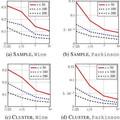
Figure 2: Relative errors (y-axis) v.s. #landmarksn(x-axis) for varying dimensionr;nexpressed as multiples ofr.

cj :=c(g(xj), yj)is

∇Wcj =∇g(xj)c(g(xj), yj)·xj

· −sin(W>xj)α1+ cos(W>xj)α2

>

,

whereα1,α2 ∈ Rr denote the firstrentries (cosine part) and the secondrentries (sine part) ofα, respectively. Hence the gradient descent update for W is W ← W −µ ·

1

N PN

j=1∇Wcj+η· ∇WL

. Overall, the time complexity of each gradient descent step forα,β, andWisO(N dr), which is linear in the sample size.

Recently, Sinha and Duchi (2016) proposed to learn fea-ture weightspj’s by kernel alignment; Yu et al. (2015) con-sidered optimizing spectral sampleswj’s using classifica-tion loss. There are two key differences between our work and theirs. First, previous works learn eitherpj’s orwj’s,

while we adjust both. Second, we employ a hybrid loss in-corporating EKAL minimization as a novel regularization to the learned model, leading to improved generalization.

Experiments

This section reports empirical evaluations in numerical ker-nel matrix approximation and supervised learning tasks. We denote our Fourier features learned by minimizing EKAL (Algorithm 1) with sampling and clustering as SAMPLEand CLUSTER, respectively. In supervised learning tasks, we minimize hybrid loss with sampling-based EKAL and name it SUPERVISE. We have compared with the following meth-ods for constructing Fourier features:

◦ MC: Standard Monte Carlo sampling for random Fourier features (Rahimi and Recht 2008)

◦ FASTFOOD: Fast sampling using Hadamard matrices (Le, Sarl´os, and Smola 2013).

◦ HALTON, SOBOL, LATTICE, DIGIT: 4 low-discrepancy sequences used in QMC sampling (Yang et al. 2014).

◦ MM: The moment matching approach (Shen, Yang, and Wang 2017).

◦ WEIGHT: Learning feature weights for kernel approxima-tion via linear ridge regression (Chang et al. 2017).

◦ ALIGN: Kernel learning via alignment maximization (Sinha and Duchi 2016).

The benchmark datasets used are listed in Table 1. For simplicity, we convertCovtypeandMNISTto binary clas-sification (type 1 vs. not type 1, and digit0vs. digit1). All data samples are split into training/test sets (2 : 1), unless provided in the original data. We tune the parameters via cross validation on training set. Input data is normalized to have zero mean and unit variance in each dimension, and the Gaussian kernel width2σ2_{is chosen as the dimensiondof}

the input data, equal toE[kx1−x2k2/2]after normalization.

Two-Dimensional Toy Examples

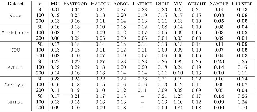
Table 2: Relative kernel approximation errors. The errors of LATTICEforMNISTare missing because the code provided by (Yang et al. 2014) cannot generate a lattice sequence of dimension larger than250.

Dataset r MC FASTFOOD HALTON SOBOL LATTICE DIGIT MM WEIGHT SAMPLE CLUSTER

Wine

50 0.31 0.34 0.24 0.27 0.28 0.23 0.25 0.24 0.14 0.13 100 0.19 0.25 0.18 0.20 0.19 0.15 0.17 0.15 0.08 0.08 200 0.13 0.16 0.11 0.14 0.13 0.11 0.13 0.10 0.05 0.05

Parkinson

50 0.16 0.13 0.10 0.18 0.12 0.08 0.14 0.10 0.05 0.04 100 0.08 0.14 0.09 0.12 0.07 0.05 0.09 0.05 0.03 0.02 200 0.06 0.08 0.05 0.09 0.06 0.04 0.05 0.03 0.02 0.01

CPU

50 0.17 0.18 0.14 0.18 0.14 0.13 0.13 0.14 0.11 0.09 100 0.13 0.13 0.11 0.12 0.11 0.09 0.09 0.10 0.07 0.05 200 0.08 0.10 0.07 0.09 0.07 0.06 0.06 0.06 0.04 0.03

Adult

50 0.27 0.29 0.27 0.28 0.28 0.26 0.89 0.26 0.23 0.25

100 0.19 0.22 0.18 0.20 0.20 0.18 0.24 0.19 0.14 0.16

200 0.14 0.16 0.13 0.14 0.14 0.11 0.10 0.13 0.10 0.11

Covtype

50 0.23 0.25 0.22 0.22 0.23 0.21 0.19 0.22 0.16 0.14 100 0.16 0.18 0.15 0.16 0.16 0.13 0.12 0.14 0.09 0.07 200 0.11 0.12 0.10 0.12 0.11 0.09 0.09 0.09 0.05 0.04

MNIST

50 0.17 0.21 0.17 0.18 – 0.21 1.25 0.17 0.14 0.26

100 0.13 0.15 0.13 0.13 – 0.13 1.10 0.12 0.09 0.24

200 0.09 0.10 0.09 0.08 – 0.09 0.84 0.08 0.06 0.10

Table 3: Generalization error for regression (RMSE) and classification (%). Shaded methods use labels in computing features.

Dataset MC FASTFOODHALTONSOBOLLATTICEDIGIT MM WEIGHT ALIGN SAMPLECLUSTER SUPERVISE

Wine 0.712 0.697 0.697 0.707 0.709 0.703 0.716 0.710 0.703 0.706 0.703 0.697

Parkinson6.931 6.929 6.963 6.898 6.959 6.997 6.946 6.950 6.895 6.957 6.931 6.432

CPU 7.238 6.632 7.196 7.471 6.455 7.415 7.664 7.533 6.889 7.495 7.060 3.687

Adult 16.02 15.91 16.01 15.90 15.94 15.87 15.75 16.10 15.94 15.98 15.96 15.64

Covtype 19.37 19.94 19.39 19.63 19.39 19.95 19.78 19.67 19.46 19.52 19.32 19.78 MNIST 0.757 0.757 0.567 0.615 – 0.709 0.378 0.851 0.662 0.757 0.735 0.378

their weightspj’s) and input data distributionP(x). For vi-sualization purpose,wj’s are chosen from a uniform grid and onlypj’s are optimized (in real-data experiments,wj’s andpj’s are optimized together). Note that the color-coded weight map can be deemed intuitively as an “distribution sensitive” importance distribution in the spectral domain.

Kernel Approximation Experiments

We use the relative errorkKe −KkF/kKkFto quantify the performance of kernel approximation, whereKis the exact kernel, andK˜ the approximate one by Algorithm 1.

Number of Landmarks in EKAL-Approximators.We first explore the number of landmarks in the EKAL-approximators that guarantees accurate result on the entire data. For number of features r = 50, 100, and 200, we run SAMPLE and CLUSTERp with number of landmarks

n = r/25, r/5,r, and 5r. Errors are shown in Figure 2. Clearly, one achieves relatively small generalization error fornas small asr. So we fixn=rfor the rest experiments.

Relative Approximation Errors. We reportp relative kernel approximation errors of all competing algorithms on six benchmark datasets forr = 50,100,200 (Table 2). In each dataset, at least one of our two methods, SAMPLEand CLUSTER, achieves the lowest error. This demonstrates the

advantage learned Fourier features in kernel approximation. Usually, CLUSTERperforms better than SAMPLE, mean-ing that landmarks chosen as cluster centers yield better ker-nel approximation. However, when the number of landmarks

nis lower than the input dimension (n ≤200 < 784 =d

forMNIST), CLUSTERbecomes worse than SAMPLE. This is because when the number of clusters is too small, the clus-ter cenclus-ters can be undesirably far from the actual input sam-ples. In such a case, replacing the cluster centers with their closest samples proves an effective cure. Due to the space limit, we defer the empirical study of the performance of the modified EKAL approximator (that uses the closest samples to the cluster centers as landmarks) to an extended version of this paper. Indeed, such modification improves the perfor-mance of CLUSTERin high-dimensional cases, and achieves competitive performance against both CLUSTERand SAM -PLEfor all datasets.

Supervised Learning Experiments

error. All the experiments usen=r= 200.

The regression or classification results on six benchmark datasets are reported in Table 3. When comparing meth-ods that do not use label information in constructing the Fourier features (methods not shaded in Table 3), the results are inconclusive, i.e., any method performs better on certain tasks and worse on others. Overall, the unsupervised features learned by our methods (SAMPLE and CLUSTER) are quite comparable to others. When labels are used in constructing the Fourier features, our method (SUPERVISE) attains lowest generalization error on most datasets, demonstrating its su-periority over both unsupervised feature construction meth-ods and recently proposed, supervised method (ALIGN).

Conclusion

In this paper, we propose a novel framework for learning Fourier features that adapt to input data. Both spectral sam-ples and weights are optimized jointly, which can be further engaged in any supervised learning framework. Extensive theoretical/empirical results demonstrate advantages of our method. In the future, we will study theoretic connections between the proposed Fourier features and explicit kernel low-rank decomposition.

Acknowledgement

Jun Wang is supported in part by the National Science Foun-dation of China NO.61672236.

References

Avron, H.; Sindhwani, V.; Yang, J.; and Mahoney, M. W. 2016. Quasi-monte carlo feature maps for shift-invariant kernels.Journal of Machine Learning Research17(120):1–38.

Avron, H.; Sindhwani, V.; and Woodruff, D. 2013. Sketching struc-tured matrices for faster nonlinear regression. InAdvances in Neu-ral Information Processing Systems, 2994–3002.

Bach, F. 2017. On the equivalence between kernel quadrature rules and random feature expansions.Journal of Machine Learning Research18(21):1–38.

Barber, D. 2012.Bayesian reasoning and machine learning. Cam-bridge University Press.

Chang, W.-C.; Li, C.-L.; Yang, Y.; and P´oczos, B. 2017. Data-driven random fourier features using stein effect. InProceedings of the Twenty-Sixth International Joint Conference on Artificial In-telligence, 1497–1503.

Cortes, C.; Mohri, M.; and Talwalkar, A. 2010. On the impact of kernel approximation on learning accuracy. InProceedings of the Thirteenth International Conference on Artificial Intelligence and Statistics, 113–120.

Drineas, P., and Mahoney, M. W. 2005. On the nystr¨om method for approximating a gram matrix for improved kernel-based learning.

Journal of Machine Learning Research6(Dec):2153–2175. Fowlkes, C.; Belongie, S.; Chung, F.; and Malik, J. 2004. Spectral grouping using the nystrom method.IEEE Transactions on Pattern Analysis and Machine Intelligence26(2):214–225.

Gine, E., and Zinn, J. 1984. Some limit theorems for empirical processes.The Annals of Probability12(4):929–989.

Halko, N.; Martinsson, P. G.; and Tropp, J. A. 2011. Finding struc-ture with randomness: Probabilistic algorithms for constructing ap-proximate matrix decompositions.SIAM Review53(2):217–288.

Kumar, S.; Mohri, M.; and Talwalkar, A. 2012. Sampling methods for the nystr¨om method. Journal of Machine Learning Research

13(Apr):981–1006.

Le, Q.; Sarl´os, T.; and Smola, A. 2013. Fastfood-approximating kernel expansions in loglinear time. InProceedings of the Interna-tional Conference on Machine Learning, volume 85.

Lucas, ´E. 1883. Les jeux de demoiselles. In R´ecr´eations Math´ematiques. Gauthier-Villars (Paris). 161–197.

Mahoney, M. W. 2011. Randomized algorithms for matrices and data. Foundations and TrendsR in Machine Learning3(2):123– 224.

Massart, P. 2000. Some applications of concentration inequali-ties to statistics. Annales de la Facult´e des sciences de Toulouse : Math´ematiques9(2):245–303.

McDiarmid, C. 1989. On the method of bounded differences. Sur-veys in combinatorics141(1):148–188.

Pennington, J.; Felix, X. Y.; and Kumar, S. 2015. Spherical random features for polynomial kernels. InAdvances in Neural Information Processing Systems, 1846–1854.

Rahimi, A., and Recht, B. 2008. Random features for large-scale kernel machines. InAdvances in Neural Information Processing Systems, 1177–1184.

Sch¨olkopf, B., and Smola, A. J. 2002. Learning with kernels: support vector machines, regularization, optimization, and beyond. MIT press.

Shen, W.; Yang, Z.; and Wang, J. 2017. Random features for shift-invariant kernels with moment matching. InProceedings of the Thirty-First AAAI Conference on Artificial Intelligence.

Si, S.; Hsieh, C.-J.; and Dhillon, I. 2014. Memory efficient kernel approximation. InProceedings of the 31st International Confer-ence on Machine Learning, volume 32 ofProceedings of Machine Learning Research, 701–709. PMLR.

Sinha, A., and Duchi, J. C. 2016. Learning kernels with random features. InAdvances in Neural Information Processing Systems, 1298–1306.

Vedaldi, A., and Zisserman, A. 2012. Efficient additive kernels via explicit feature maps. IEEE Transactions on Pattern Analysis and Machine Intelligence34(3):480–492.

Williams, C. K., and Seeger, M. 2001. Using the nystr¨om method to speed up kernel machines. InAdvances in Neural Information Processing Systems, 682–688.

Woodruff, D. P., et al. 2014. Sketching as a tool for numerical linear algebra.Foundations and TrendsR in Theoretical Computer

Science10(1–2):1–157.

Yang, J.; Sindhwani, V.; Avron, H.; and Mahoney, M. 2014. Quasi-monte carlo feature maps for shift-invariant kernels. In Proceed-ings of the 31st International Conference on Machine Learning, 485–493.