A General Distributed Dual Coordinate Optimization
Framework for Regularized Loss Minimization
Shun Zheng∗ [email protected]
Institute for Interdisciplinary Information Sciences Tsinghua University
Beijing, China
Jialei Wang [email protected]
Department of Computer Science The University of Chicago Chicago, Illinois
Fen Xia [email protected]
Beijing Wisdom Uranium Technology Co., Ltd. Beijing, China
Wei Xu [email protected]
Institute for Interdisciplinary Information Sciences Tsinghua University
Beijing, China
Tong Zhang [email protected]
Tencent AI Lab Shenzhen, China
Editor:Sathiya Keerthi
Abstract
In modern large-scale machine learning applications, the training data are often parti-tioned and stored on multiple machines. It is customary to employ the “data parallelism” approach, where the aggregated training loss is minimized without moving data across machines. In this paper, we introduce a novel distributed dual formulation for regularized loss minimization problems that can directly handle data parallelism in the distributed setting. This formulation allows us to systematically derive dual coordinate optimization procedures, which we refer to asDistributed Alternating Dual Maximization(DADM). The framework extends earlier studies described in (Boyd et al., 2011; Ma et al., 2017; Jaggi et al., 2014; Yang, 2013) and has rigorous theoretical analyses. Moreover, with the help of the new formulation, we develop the accelerated version of DADM (Acc-DADM) by gener-alizing the acceleration technique from (Shalev-Shwartz and Zhang, 2014) to the distributed setting. We also provide theoretical results for the proposed accelerated version, and the new result improves previous ones (Yang, 2013; Ma et al., 2017) whose iteration complex-ities grow linearly on the condition number. Our empirical studies validate our theory and show that our accelerated approach significantly improves the previous state-of-the-art distributed dual coordinate optimization algorithms.
∗. Most of the work was done during the internship of Shun Zheng at Baidu Big Data Lab in Beijing.
c
Keywords: distributed optimization, stochastic dual coordinate ascent, acceleration, regularized loss minimization, computational complexity
1. Introduction
In large-scale machine learning applications for big data analysis, it becomes a common practice to partition the training data and store them on multiple machines connected via a commodity network. A typical setting of distributed machine learning is to allow these machines to train in parallel, with each machine processing its local data with no
data communication. This paradigm is often referred to as data parallelism. To reduce
the overall training time, it is often necessary to increase the number of machines and to minimize the communication overhead. A significant challenge is to reduce the training time as much as possible when we increase the number of machines. A practical solution requires two research directions: one is to improve the underlying system design making it suitable for machine learning algorithms (Dean and Ghemawat, 2008; Zaharia et al., 2012; Dean et al., 2012; Li et al., 2014); the other is to adapt traditional single-machine optimization methods to handle data parallelism (Boyd et al., 2011; Yang, 2013; Mahajan et al., 2013;
Shamir et al., 2014; Jaggi et al., 2014; Mahajan et al., 2017; Ma et al., 2017; Tak´aˇc et al.,
2015; Zhang and Lin, 2015). This paper focuses on the latter.
For big data machine learning on a single machine, there are two types of algorithms: batch algorithms such as gradient descent or L-BFGS (Liu and Nocedal, 1989), and stochas-tic optimization algorithms such as stochasstochas-tic gradient descent and their modern variance reduced versions (Defazio et al., 2014; Johnson and Zhang, 2013). It is known that batch algorithms are relatively easy to parallelize. However, on a single machine, they converge more slowly than the modern stochastic optimization algorithms due to their high per-iteration computation costs. Specifically, it has been shown that the modern stochastic optimization algorithms converge faster than the traditional batch algorithms for convex regularized loss minimization problems. The faster convergence can be guaranteed in theory and observed in practice.
The fast convergence of modern stochastic optimization methods has led to studies
to extend these methods to the distributed computing setting. Specifically, this paper
considers the generalization of Stochastic Dual Coordinate Ascent (SDCA) method (Hsieh et al., 2008; Shalev-Shwartz and Zhang, 2013) and its proximal variant (Shalev-Shwartz and Zhang, 2014) to handle distributed training using data parallelism. Although this problem has been considered previously (Yang, 2013; Jaggi et al., 2014; Ma et al., 2017), these earlier approaches work with the dual formulation that is the same as the traditional single-machine dual formulation, where dual variables are coupled, and hence run into difficulties when they try to motivate and analyze the derived methods under the distributed environment.
One contribution of this work is to introduce a new dual formulation specifically for distributed regularized loss minimization problems when data are distributed to multiple machines. In our new formulation, we decouple the local dual variables through
introduc-ing another dual variable β. This unique dual formulation allows us to naturally extend
formu-lation, leading to new theoretical results. This new dual formulation can also be combined with the acceleration technique of (Shalev-Shwartz and Zhang, 2014) to further improve convergence.
In the proposed formulation, each iteration of the distributed dual coordinate ascent optimization is naturally decomposed into a local step and a global step. In the local step, we allow the use of any local procedure to optimize a local dual objective function using local parameters and local data on each machine. This flexibility is similar to those of (Ma et al., 2017; Jaggi et al., 2014). For example, we may apply ProxSDCA as the local procedure. In the local step, a computer node can perform the optimization independently without communicating with each other. While in the global step, nodes communicate with each other to synchronize the local parameters and jointly update the global primal solution. Only this global step requires communication among nodes.
We summarize our main contributions as follows:
New distributed dual formulation This new formulation naturally leads to a two-step local-global dual alternating optimization procedure for distributed machine learning. We
thus call the resulting procedureDistributed Alternating Dual Maximization(DADM). Note
that DADM directly generalizes ProxSDCA, which can handle complex regularizations such
asL2-L1 regularization.
New convergence analysis The new formulation allows us to directly generalize the analysis of ProxSDCA in (Shalev-Shwartz and Zhang, 2014) to the distributed setting. This
analysis is in contrast to that of CoCoA+ in (Ma et al., 2017), which employs a different
way based on the Θ-approximate solution assumption of the local solver. Our analysis can lead to simplified results in the commonly used mini-batch setup.
Acceleration with theoretical guarantees Based on the new distributed dual formu-lation, we can naturally derive a distributed version of the accelerated proximal SDCA method (AccProxSDCA) of (Shalev-Shwartz and Zhang, 2014), which has been shown to
be effective on a single machine. We call the resulting procedure Accelerated Distributed
Alternating Dual Maximization(Acc-DADM). The main idea is to modify the original
for-mulation using a sequence of approximations that have stronger regularizations. Moreover, we directly adapt theoretical analyses of AccProxSDCA to the distributed setting and pro-vide guarantees for Acc-DADM. Our theorems guarantee that we can always obtain a computation speedup compared with the single-machine AccProxSDCA. These guarantees improve the theoretical results of DADM and previous methods (Yang, 2013; Ma et al., 2017) whose iteration complexities grow linearly on the condition number. Latter methods possibly fail to provide computation time improvement over the single-machine ProxSDCA when the condition number is large.
We organize the rest of the paper as follows. Section 2 discusses related works. Section 3 provides preliminary definitions. Section 4 to 6 present the distributed primal formula-tion, the distributed dual formulation and our DADM method respectively. Section 7 then provides theorems for DADM. Section 8 introduces the accelerated version and provides corresponding theoretical guarantees. Section 9 includes all proofs of this paper. Section 10 provides extensive empirical studies of our novel method. Finally, Section 11 concludes the whole paper.
2. Related Work
Several generalizations of SDCA to the distributed settings have been proposed in the
literature, including DisDCA (Yang, 2013), CoCoA (Jaggi et al., 2014), and CoCoA+ (Ma
et al., 2017).
DisDCA was the first attempt to study distributed SDCA, and it provided a basic theoretical analysis and a practical variant that behaves well empirically. Nevertheless, their theoretical result only applies to a few specially chosen mini-batch local dual updates that differ from the practical method used in their experiments. In particular, they did not show that optimizing each local dual problem leads to convergence. This limitation makes the methods they analyzed inflexible.
CoCoA was proposed to fix the above gap between theory and practice, and it was claimed to be a framework for distributed dual coordinate ascent in that it allows any local dual solver to be used for the local dual problem, rather than the impractical choices of DisDCA. However, the actual performance of CoCoA is inferior to the practical variant proposed in DisDCA with an aggressive local update. We note that the practical variant of DisDCA did not have a solid theoretical guarantee at that time.
CoCoA+ fixed this situation and may be regarded as a generalization of CoCoA. The
most effective choice of the aggregation parameter leads to a version which is similar to DisDCA, but allows exact optimization of each dual problem in their theory. According to
studies in (Ma et al., 2017), the resulting CoCoA+ algorithm performs significantly better
than the original CoCoA both theoretically and empirically. The original CoCoA+ (Ma
et al., 2015) can only handle problems with the L2 regularizer, and it was generalized to
general strongly convex regularizers in the long version (Ma et al., 2017). Besides, (Smith et al., 2016) extended the framework to solve the primal problem of regularized loss
min-imization and cover general non-strongly convex regularizers such as L1 regularizer, and
(Hsieh et al., 2015) studied parallel SDCA with asynchronous updates.
Although CoCoA+ has the advantage of allowing arbitrary local solvers and flexible
approximate solutions of local dual problems, its theoretical analyses do not capture the contribution of the number of machines and the mini-batch size to the iteration complexity
explicitly. Moreover, the iteration complexities of both CoCoA+ and DisDCA grow
lin-early with the condition number. Thus they probably cannot provide computation time improvement over the single-machine SDCA when the condition number is large. This pa-per will remedy these unsatisfied aspects by providing a different analysis based on a new distributed dual formulation. Using this formulation, we can analyze procedures that can
take an arbitrary local dual solver, which is like CoCoA+; moreover, we allow the dual
us to naturally generalize AccProxSDCA and relevant theoretical results to the distributed setting. Our empirical results also validate the superiority of the accelerated approach.
While we focus on extending SDCA in this paper, we note that there are other ap-proaches for parallel optimization. For example, there are direct attempts to parallelize stochastic gradient descent (Niu et al., 2011; Zinkevich et al., 2010). Some of these pro-cedures only consider multi-core shared memory situation, which is very different from the distributed computing environment investigated in this paper. In the setting of dis-tributed computing, data are partitioned into multiple machines, and one often needs to study communication-efficient algorithms. In such cases, one extreme is to allow exact opti-mization of subproblems on each local machine as considered in (Shamir et al., 2014; Zhang and Lin, 2015). Although this approach minimizes communication, the computation cost for each local solver can dominate the overall training. Therefore in practice, it is
neces-sary to do a trade-off by using the mini-batch update approach (Tak´aˇc et al., 2013, 2015).
However, it is difficult for traditional mini-batch methods to design reasonable aggregation
strategies to achieve fast convergence. (Tak´aˇc et al., 2015) studied how the step size can be
reduced when the mini-batch size grows in the distributed setting. (Lee and Roth, 2015) derived an analytical solution of the optimal step size for dual linear support vector machine problems. Besides, (Mahajan et al., 2013) presented a general framework for distributed optimization based on local functional approximation, which include several first-order and second-order methods as special cases. (Mahajan et al., 2017) considered each machine to handle a block of coordinates and proposed distributed block coordinate descent methods
for solving`1 regularized loss minimization problems.
Different from those methods,Distributed Alternating Dual Maximization(DADM)
pro-posed in this work handles the traoff between computation and communication by de-veloping bounds for mini-batch dual updates, which is similar to (Yang, 2013). Moreover, DADM allows other better local solvers to achieve faster convergence in practice.
3. Preliminaries
In this section, we introduce some notations used later. All functions that we consider in this paper are proper convex functions over a Euclidean space.
Given a function f :Rd→R, we denote its conjugate functionas
f∗(b) = sup
a
[b>a−f(a)].
A function f :Rd→RisL-Lipschitz with respect tok · k2 if for alla, b∈Rd, we have
|f(a)−f(b)| ≤Lka−bk2.
A function f :Rd→Ris (1/γ)-smooth with respect tok · k2 if it is differentiable and
its gradient is (1/γ)-Lipschitz with respect to k · k2. An equivalent definition is that for all
a, b∈Rd, we have
f(b)≤f(a) +∇f(a)>(b−a) + 1
2γkb−ak 2 2.
A function f :Rd→Risλ-strongly convexwith respect tok · k2 if for anya, b∈Rd,
we have
f(b)≥f(a) +∇f(a)>(b−a) + λ
2kb−ak
where∇f(a) is any subgradient off(a).
It is well known that a functionf isγ-strongly convex with respect to k · k2 if and only
if its conjugate functionf∗ is (1/γ)-smooth with respect tok · k2.
4. Distributed Primal Formulation
In this paper, we consider the following generic regularized loss minimization problem:
min
w∈Rd
"
P(w) :=
n
X
i=1
φi(Xi>w) +λng(w) +h(w)
#
, (1)
which is often encountered in practical machine learning problems. Here we assume each
Xi ∈ Rd×q is a d×q matrix, w ∈ Rd is the model parameter vector, φi(u) is a convex
loss function defined on Rq, which is associated with the i-th data point, λ > 0 is the
regularization parameter,g(w) is a strongly convex regularizer and h(w) is another convex
regularizer. A special case is to simply set h(w) = 0. Here we allow the more general
formulation, which can be used to derive different distributed dual forms that may be useful for special purposes.
The above optimization formulation can be specialized to a variety of machine learning
problems. As an example, we may consider the L2-L1 regularized least squares problem,
whereφi(x>i w) = (w>xi−yi)2 for vector input dataxi ∈Rdand real valued outputyi∈R, g(w) =kwk2
2+akwk1, and h(w) =bkwk1 for somea, b≥0.
If we seth(w) = 0, then it is well-known (see, for example, (Shalev-Shwartz and Zhang,
2014)) that the primal problem (1) has an equivalent single-machine dual form of
max
α∈Rn
"
D(α) :=−
n
X
i=1
φ∗i(−αi)−λng∗
Pn
i=1Xiαi λn
#
, (2)
whereα= [α1,· · · , αn], αi ∈Rq (i= 1, ..., n) are dual variables, φ∗i is the convex conjugate
function of φi, and similarly, g∗ is the convex conjugate function of g.
The stochastic dual coordinate ascent method, referred to as SDCA in (Shalev-Shwartz and Zhang, 2014), maximizes the dual formulation (2) by optimizing one randomly cho-sen dual variable at each iteration. Throughout the algorithm, the following primal-dual relationship is maintained:
w(α) =∇g∗
Pn
i=1Xiαi λn
, (3)
for some subgradient ∇g∗(v).
It is known that w(α∗) = w∗, where w∗ and α∗ are optimal solutions of the primal
problem and the dual problem respectively. It was shown in (Shalev-Shwartz and Zhang,
2014) that the duality gap defined as P(w(α))−D(α), which is an upper-bound of the
primal sub-optimality P(w(α))−P(w∗), converges to zero. Moreover, a convergence rate
generalize the single-machine dual formulation (2) to the distributed setting, and study the corresponding distributed version of SDCA.
In the distributed setting, we assume that the training data are partitioned and
dis-tributed tom machines. In other words, the index setS ={1, ..., n} of the training data is
divided into m non-overlapping partitions, where each machine` ∈ {1, ..., m} contains its
own partition S` ⊆S. We assume that ∪`S`=S, and we use n` :=|S`|to denote the size
of the training data on machine `.
Next, we can rewrite the primal problem (1) as the following constrained minimization problem that is suitable for the multi-machine distributed setting:
min
w;{w`}m`=1
m
X
`=1
P`(w`) +h(w)
s.t. w`=w, for all `∈ {1, ..., m},
where P`(w`) :=
X
i∈S`
φi(Xi>w`) +λn`g(w`),
(4)
where w` represents the local primal variable on each machine `, P` is the corresponding
local primal problem and the constraintsw` =ware imposed to synchronize the local primal
variables. Obviously this multi-machine distributed primal formulation (4) is equivalent to the original primal problem (1).
We note that the idea of objective splitting in (4) is similar to the global variable con-sensus formulation described in (Boyd et al., 2011). Instead of using the commonly used ADMM (Alternating Direction Method of Multipliers) method that is not a generalization of (2), in this paper we derive a distributed dual formulation based on (4) that directly generalizes (2). We further propose a framework called Distributed Alternating Dual Max-imization (DADM) to solve the distributed dual formulation. One advantage of DADM over ADMM is that DADM does not need to solve the subproblems in high accuracy, and thus it can naturally enjoy the trade-off between computation and communication, which
is similar to related methods such as DisDCA, CoCoA and CoCoA+.
5. Distributed Dual Formulation
The optimization problem (4) can be further rewritten as:
min
w;{w`};{ui}
m
X
`=1
X
i∈S`
φi(ui) +λn`g(w`)
+h(w)
s.t ui=Xi>w`, for all i∈S` w`=w, for all`∈ {1, ..., m}.
(5)
Here we introducendual variablesα:={αi}ni=1, where eachαiis the Lagrange multiplier
for the constraintui−Xi>w`= 0, and mdual variables β:={β`}m`=1, where eachβ` is the
objective function with Lagrange multipliers as follows:
J(w;{w`};{ui};{αi};{β`})
:=
m
X
`=1
X
i∈S`
φi(ui) +α>i (ui−Xi>w`)
+λn`g(w`) +β`>(w`−w)
+h(w).
Proposition 1 Define the dual objective as
D(α, β) :=
m
X
`=1
X
i∈S`
−φ∗i(−αi)−λn`g∗
P
i∈S`Xiαi−β`
λn`
−h∗ X
` β`
!
.
Then we have
D(α, β) = min
w;{w`};{ui}
J(w;{w`};{ui};{αi};{β`}),
where the minimizers are achieved when the following equations are satisfied
∇φi(ui) +αi=0,
−
X
i∈S`
Xiαi−β`
+λn`∇g(w`) =0,
−X
`
β`+∇h(w) =0,
(6)
for some subgradients ∇φi(ui), ∇g(w`), and ∇h(w).
When β = {β`} are fixed, we may define the local single-machine dual formulation on
each machine `with respect to α(`) as
˜
D`(α(`)|β`) :=
X
i∈S`
−φ∗i(−αi)−λn`g∗
P
i∈S`Xiαi−β`
λn`
, (7)
where α(`) represents local dual variables {αi;i ∈ S`} on machine `, β` ∈ Rd serves as a
carrier for synchronization of machine `. Based on Proposition 1, we obtain the following
multi-machine distributed dual formulation for the corresponding primal problem (4):
D(α, β) =
m
X
`=1
˜
D`(α(`)|β`)−h∗ m
X
`=1 β`
!
. (8)
Moreover, we have the non-negative duality gap, and zero duality gap can be achieved
when wis the minimizer of P(w) and (α, β) maximizes the dualD(α, β).
Proposition 2 Given any (w, α, β), the following duality gap is non-negative:
P(w)−D(α, β)≥0.
Moreover, zero duality gap can be achieved at (w∗, α∗, β∗), where w∗ is the minimizer of
We note that the parameters {β`}m`=1 pass the global information across multiple
ma-chines. When β` is fixed, ˜D`(α(`)|β`) with respect to α(`) corresponds to the dual of the
adjusted local primal problem:
˜
P`(w`|β`) :=
X
i∈S`
φi(Xi>w`) +λn`g˜`(w`), (9)
where the original regularizer λn`g(w`) in P`(w`) is replaced by the adjusted regularizer
λn`˜g`(w`) :=λn`g(w`) +β`>w`.
Similar to the single-machine primal-dual relationship of (3), we have the following local primal-dual relationship on each machine as:
w`(α(`), β`) =∇g∗(˜v`) =∇g˜`∗(v`), (10)
where
v` =
P
i∈S`Xiαi
λn`
, ˜v` =v`− β` λn`
.
Moreover, we can define the global primal-dual relationship as
w(α, β) =∇g∗(˜v) =∇g˜∗(v), (11)
where
v=
Pn
i=1Xiαi
λn , ˜v=v−
P
`β` λn .
We can also establish the relationship of global-local duality in Proposition 3.
Proposition 3 Given (w, α, β) and {w`} such that w1 = · · · = wm = w, we have the
following decomposition of global duality gap as the sum of local duality gaps:
P(w)−D(α, β)≥
m
X
`=1
h
˜
P`(w`|β`)−D˜`(α(`)|β`)
i
,
and the equality holds when∇h(w) =P
`β` for some subgradient ∇h(w).
Although we allow arbitrary h(w), the case of h(w) = 0 is of special interests. This
corresponds to the conjugate function
h∗(β) =
(
+∞ ifβ6= 0
0 ifβ= 0.
That is, the termh∗(Pm
`=1β`) is equivalent to imposing the constraint
Pm
Algorithm 1 Local Dual Update
Retrieve local parameters (α(`t−1),˜v`(t−1))
Randomly pick a mini-batch Q`⊂S`
Approximately maximize (12) w.r.t ∆αQ`
Update α(it) asα(it)=α(it−1)+ ∆αi for all i∈Q` return ∆v(`t)= λn1
`
P
i∈Q`Xi∆αi
6. Distributed Alternating Dual Maximization
Minimizing the primal formulation (4) is equivalent to maximizing the dual formulation (8), and the latter can be achieved by repeatedly using the following alternating optimization
strategy, which we refer to asDistributedAlternatingDualMaximization (DADM):
• Local step: fixβ` and let each machine approximately optimize ˜D`(α(`)|β`) w.r.tα(`)
in parallel.
• Global step: maximize the global dual objective w.r.t β`, and set the global primal
parameterw accordingly.
The above steps are applied in iterations t = 1,2, . . . , T. At the beginning of each
iteration t, we assume that the local primal and dual variables on each local machine are
(α((t`−)1), β`(t−1), v`(t−1)), then we seek to update α((t`−)1) to α((t`)) and v`(t−1) tov`(t) in the local step, and seek to updateβ`(t−1) toβ`(t) in the global step.
We note that the local step can be executed in parallel w.r.t dual variables {α(`)}m`=1.
In practice, it is often useful to optimize (7) approximately by using a randomly selected
mini-batch Q` ⊂ S` of size |Q`| = M`. That is, we want to find ∆α(it) with i ∈ Q` to
approximately maximize the local dual objective as follows:
˜
D(Qt)
`(∆αQ`) :=−
X
i∈Q`
φ∗i(−αi(t−1)−∆αi)−λn`g∗
˜
v(`t−1)+
P
i∈Q`Xi∆αi
λn`
. (12)
This step is described in Algorithm 1. We can use any solver for this approximate optimization, and in our experiments, we choose ProxSDCA.
The global step is to synchronize all local solutions, which requires communication among the machines. This is achieved by optimizing the following dual objective with respect to all β={β`}:
β(t) ∈arg max
β D(α
(t), β). (13)
Proposition 4 Givenv, letw(v) be the unique solution of the following optimization prob-lem
w(v) = arg min
w
h
−λnw>v+λng(w) +h(w)
i
(14)
that satisfies
for some subgradients ∇g(w) and ∇h(w) =ρ atw=w(v). Then β¯(v) =ρ is a solution of
max
b
−λng∗
v− b
λn
−h∗(b)
,
and
w(v) =∇g∗
v−β¯(v)
λn
.
Proposition 5 Given α, a solution of
max
β D(α, β)
can be obtained by setting
β` =λn`
v`(α(`))−v(α) +
¯
β(v(α))
λn
where β¯(v(α)) is defined in Proposition 4,
v(α) =
Pn
i=1Xiαi
λn , v`(α(`)) =
P
i∈S`Xiαi
λn` .
Moreover, if we let
w=w(α, β) =w(v(α)) =∇g∗
v(α)−β¯(v(α))
λn
,
where w(v) is defined in Proposition 4, and
w`=w`(α(`), β`) =∇g∗
v`(α(`))− β` λn`
,
thenw=w` for all`, and
P(w)−D(α, β) =
m
X
`=1
[ ˜P`(w`|β`)−D˜`(α(`)|β`)].
According to Proposition 5, the solution of (13) is given by
β`(t)=λn` v (t) ` −v
(t)+ρ(t) λn
!
,
where
v(t)=
m
X
`=1 n`
nv (t) ` =v
(t−1)+ m
X
`=1 n`
Algorithm 2 Distributed Alternating Dual Maximization (DADM)
Input: ObjectiveP(w), target duality gap , warm start variables winit, αinit, βinit, vinit, (if not specified, set winit= 0, αinit= 0, βinit= 0, vinit = 0), .
Initialize: letw(0)=winit,α(0)=αinit,β(0) =βinit,v(0) =vinit.
for t= 1,2, ...do
(Local step)
for all machines`= 1,2, ..., min parallel do
call an arbitrary local procedure, such as Algorithm 1
end for
(Global step)
Aggregatev(t)=v(t−1)+Pm
`=1 n`
n∆v (t) `
Compute ˜v(t) according to (15)
Let ∆˜v(t)= ˜v(t)−v˜(t−1)
for all machines`= 1,2, ..., min parallel do
update local parameter ˜v`(t)= ˜v`(t−1)+ ∆˜v(t) end for
Stopping condition: Stop ifP(w(t))−D(α(t), β(t))≤. end for
return w(t)=∇g∗(˜v(t)),α(t),β(t),v(t), and the duality gapP(w(t))−D(α(t), β(t)).
and ρ(t)=∇h(w(t)) is a subgradient ofh at the solutionw(t) of
w(t)= arg min
w
h
−λnw>v(t)+λng(w) +h(w)i,
that can achieve the first order optimality condition
−λnv(t)+λn∇g(w(t)) +ρ(t)= 0
for some subgradient ∇g(w(t)).
The definition of ˜v implies that after each global update, we have
˜
v`(t)= ˜v(t)=v(t)−ρ
(t)
λn =∇g(w
(t)), for all`= 1, . . . , m. (15)
Since the objective (12) for the local step on each machine only depends on the
mini-batch Q` (sampled from S`) and the vector ˜v(`t), which needs to be synchronized at each
global step, we know from (15) that at each timet, we can pass the same vector ˜v(t)as ˜v`(t)
to all nodes. In practice, it may be beneficial to pass ∆˜v(t) instead, especially when ∆˜v(t)
is sparse but ˜v(t) is dense. Put things together, the local-global DADM iterations can be
summarized in Algorithm 2.
If we consider the special case ofh(w) = 0, the solution of (15) is simply ˜v(`t)= ˜v(t)=v(t), and the global step in Algorithm 2 can be simplified as first aggregating updates by
∆˜v(t)= ∆v(t)=
m
X
`=1 n`
and then updating local parameters in parallel. Further, ifh(w) = 0 and the data partition
is balanced, that isn` are identical for all `= 1, . . . , m, it can be verified that the DADM
procedure (ignoring the mini-batch variation) is equivalent to CoCoA+. Therefore the
framework presented here may be regarded as an alternative interpretation.
Moreover, when the added regularization in (1) is complex and might involves more than
one non-smooth term, considering the splitting ofg(w) and h(w) can bring computational
advantages. For example, to promote both sparsity and group sparsity in the predictor we often use the sparse group lasso regularization (Friedman et al., 2010), where a combination
of L1 norm and mixed L2/L1 norm (group sparse norm) is introduced: λ1PGkwGk2 +
λ2kwk1+λ3/2kwk22, where we add a slight L2 regularization to make it strongly convex,
as did in (Shalev-Shwartz and Zhang, 2014). The proximal mapping with respect to the sparse group lasso regularization function does not have closed form solution, thus often relies on iterative minimization steps, but there are closed form proximal mapping with
respect to either L2-L1 norm or the group norm. Thus if we simply set h(w) = 0 and
λg(w) = λ1P
GkwGk2 +λ2kwk1 +λ3/2kwk22, then both the local optimization update
(12) and global synchronization step (14) will not have closed form solution. However, if
we assign the group norm on h(w) such that h(w) = λ1PGkwGk2, and hence λg(w) =
λ2kwk1 +λ3/2kwk22, the local updates steps (12) will enjoy closed form update, which
makes the implementation much easier and we only need to use iterative minimization on the (rare) global synchronization step (14).
7. Convergence Analysis
Let w∗ be the optimal solution for the primal problem P(w) and (α∗, β∗) be the optimal
solution for the dual problem D(α, β) respectively. For the primal solution w(t) and the
dual solution (α(t), β(t)) at iterationt, we define the primal sub-optimalityas
(Pt):=P(w(t))−P(w∗),
and thedual sub-optimalityas
(Dt):=D(α∗, β∗)−D(α(t), β(t)).
Due to the close relationship of the distributed dual formulation and the single-machine dual formulation, an analysis of DADM can be obtained by directly generalizing that of SDCA. We consider two kinds of loss functions, smooth loss functions that imply fast linear
convergence and general L-Lipschitz loss functions. For the following two theorems we
always assume that g is 1-strongly convex w.r.t k · k2, kXik22 ≤ R for all i, M` = |Q`|
is fixed on each machine, and our local procedure optimizes ˜DQ(t)
` sufficiently well on each
machine such that ˜D(Qt)
`(∆αQ`) ≥ ˜
D(Qt)
`(∆ ˜αQ`), where ∆ ˜αQ` is given by a special choice in
each theorem.
Theorem 6 Assume that each φi is(1/γ)-smooth w.r.tk · k2 and ∆ ˜αQ` is given by ∆ ˜αi:=s`(u
(t−1) i −α
(t−1)
where u(it−1):=−∇φi(Xi>w (t−1)
` ) ands`:=
γλn`
γλn`+M`R ∈[0,1]. To reach an expected duality gap ofE[P(w(T))−D(α(T), β(T))]≤, everyT satisfying the following condition is sufficient,
T ≥
R
γλ+ max`
n` M`
log
R
γλ+ max`
n` M`
·
(0) D
!
. (16)
Theorem 7 Assume that each φi isL-Lipschitz w.r.t k · k2, and∆ ˜αQ` is given by ∆ ˜αi:=
qn` M`
(u(it−1)−αi(t−1)), for alli∈Q`,
where −u(it−1) := ∇φi(Xi>w (t−1)
` ) and q ∈ [0,min`(M`/n`)]. To reach an expected
nor-malized duality gap of E
h
P(w)−D(α,β) n
i
≤ , every T satisfying the following condition is
sufficient,
T ≥T0+ ˜n+ G
λ ≥max
(
0,dn˜log(2λn˜
(0) D nG)e
)
+ ˜n+5G
λ, (17)
where T0 ≥ max{t0,4λG −2˜n+ t0}, t0 = max{0,dn˜log(2λn˜ (0) D
nG)e}, n˜ = max`(n`/M`), G= 4RL2, and w, α, β represent either the average vector or a randomly chosen vector of
w(t−1), α(t−1), β(t−1)overt∈ {T0+1, ..., T}respectively, such asα= T−1T0
PT
t=T0+1α
(t−1), β= 1
T−T0
PT
t=T0+1β
(t−1), w= 1 T−T0
PT
t=T0+1w
(t−1).
Remark 8 Both Theorem 6 and Theorem 7 incorporate two key components: the term
max` Mn`` and the condition number term λγ1 or L
2
λ . When the term max`
n`
M` dominates the iteration complexity, we can speed up convergence and reduce the number of communications by increasing the number of machinesm or the local mini-batch sizeM`. However, in some
circumstances when the condition number is large, it will become the leading factor, and increasing m or M` will not contribute to the computation speedup. To tackle this problem,
we develop the accelerated version of DADM in Section 8.
Remark 9 Our method is closely related to previous distributed extensions of SDCA. The-orems 6, 7 that provide theoretical guarantees for more general local updates achieve the same iteration complexity with the ones in DisDCA that only allows some special choices of local mini-batch updates. Compared with theoretical results of CoCoA+ that are based on
the Θ-approximate solution of the local dual subproblem, although the derived bounds are
within the same scale, O˜(1/) for Lipschitz losses and O˜(log(1/)) for smooth losses, our
bounds are different and complementary. The analysis of CoCoA+ can provide better
in-sights for more accurate solutions of the local sub-problems. While our analysis is based on the mini-batch setup, it can capture the contributions of the mini-batch size and the number of machines more explicitly.
Algorithm 3 Accelerated Distributed Alternating Dual Maximization (Acc-DADM).
Parameters κ,η=pλ/(λ+ 2κ), ν= (1−η)/(1 +η).
Initialize v(0) =y(0)=w(0)= 0, α(0) = 0,ξ0 = (1 +η−2)(P(0)−D(0,0)).
for t= 1,2, . . . , Touter do
1. Construct new objective:
Pt(w) = n
X
i=1
φi(Xi>w) +λng(w) +h(w) + κn
2
w−y
(t−1)
2 2.
2. Call DADM solver:
(w(t), α(t), β(t), v(t), t) = DADM(Pt,(ηξt−1)/(2 + 2η−2), w(t−1), α(t−1), β(t−1), v(t−1)).
3. Update:
y(t) =w(t)+ν(w(t)−w(t−1)).
4. Update:
ξt= (1−η/2)ξt−1.
end for
Return w(Touter).
8. Acceleration
Theorems 6, 7 all imply that when the condition number γλ1 or Lλ2 is relatively small,
DADM converges fast. However, the convergence may be slow when the condition number is large and dominates the iteration complexity. In fact, we observe empirically that the
basic DADM method converges slowly when the regularization parameter λis small. This
phenomenon is also consistent with that of SDCA for the single-machine case. In this section, we introduce the Accelerated Distributed Alternating Dual Maximization (Acc-DADM) method that can alleviate the problem.
The procedure is motivated by (Shalev-Shwartz and Zhang, 2014), which employs an
inner-outer iteration: at every iterationt, we solve a slightly modified objective, which adds
a regularization term centered around the vector
y(t−1) =w(t−1)+νw(t−1)−w(t−2), (18)
whereν ∈[0,1] is called the momentum parameter.
The accelerated DADM procedure (described in Algorithm 3) can be similarly viewed as an inner-outer algorithm, where DADM serves as the inner iteration. In the outer iteration,
we adjust the regularization vector y(t−1). That is, at each outer iteration t, we define a
modified local primal objective on each machine`, which has the same form as the original
local primal objective (9), except that ˜g`(w`) is modified to ˜g`t(w`) that is defined by
λn`˜g`t(w`) =λn`gt(w`) +β
>
` w`, λgt(w`) =λg(w`) +
κ
2kw`−y
It follows that we will need to solve a modified dual at each local step withg∗(·) replaced
bygt∗(·) in the local dual problem (12). Therefore, compared to the basic DADM procedure,
nothing changes other thang∗(·) being replaced byg∗t(·) at each iteration. Specifically, when
the number of machines m equals 1, this algorithm reduces to AccProxSDCA described
in (Shalev-Shwartz and Zhang, 2014). Thus Acc-DADM can be naturally regarded as the distributed generalization of the single-machine AccProxSDCA. Moreover, Acc-DADM also allows arbitrary local procedures as DADM does.
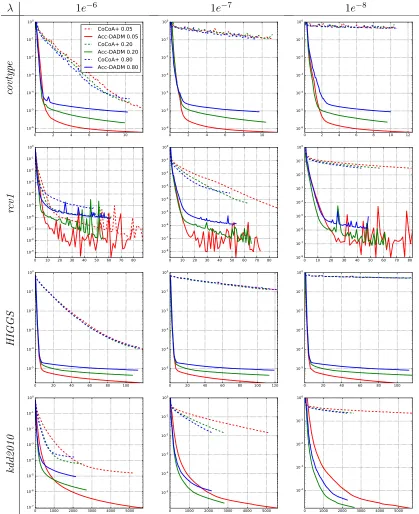
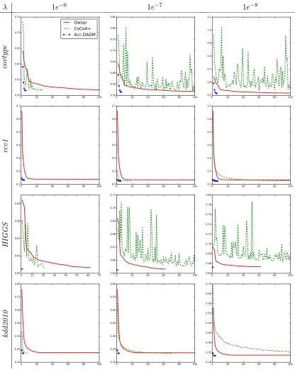
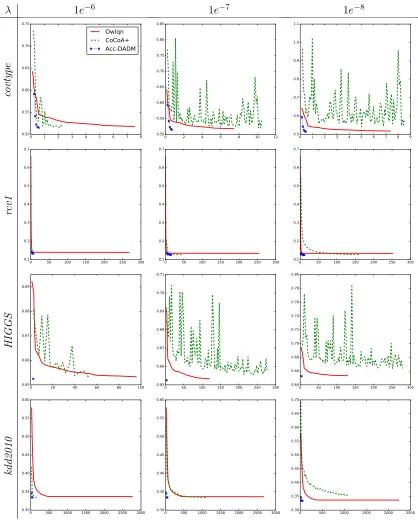
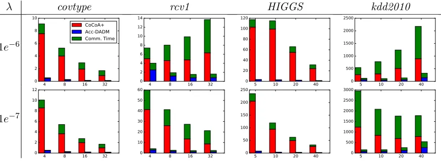
Our empirical studies show that Acc-DADM significantly outperforms DADM in many
cases. There are probably two reasons. One reason is the use of a modified regularizergt(w)
that is more strongly convex than the original regularizerg(w) whenκ is much larger than
λ. The other reason is closely related to the distributed setting considered in this paper.
Observe that in the modified local primal objective
˜
P`t(w`|β`) := ˜P`(w`|β`) +
κn`
2 kw`−y
(t−1)k2 2,
the first term corresponds to the original local primal objective and the second term is an
extra regularization due to acceleration that constrainsw`to be close toy(t−1). The effect is
that different local problems become more similar to each other, which stabilize the overall system.
8.1 Theoretical Results of Acc-DADM for Smooth Losses
The following theorem establishes the computation efficiency guarantees for Acc-DADM.
Theorem 11 Assume that eachφi is(1/γ)-smooth, andg is 1-strongly convex w.r.t k · k2,
kXik22 ≤ R for all i, M` = |Q`| is fixed on each machine. To obtain expected primal
sub-optimality:
E[P(w(t))]−P(w∗)≤,
it is sufficient to have the following number of stages in Algorithm 3
Touter≥1 +2
ηlog
ξ0
= 1 +
r
4(λ+ 2κ)
λ
log
2λ+ 2κ
λ
+ log
P(0)−D(0,0)
,
and the number of inner iterations in DADM at each stage:
Tinner ≥
R
γ(λ+κ) + max` n` M`
log
R
γ(λ+κ) + max` n` M`
+ 7 +5
2log
λ+ 2κ λ
.
In particular, suppose we assume n1 = n2 = . . . = nm, and M1 = M2 = . . . = Mm = b,
then the total vector computations for each machine are bounded by
˜
O(TouterTinnerb) = ˜O
1 +
r
κ+λ λ
!
R γ(λ+κ)+
n mb
b
!
.
and being able to obtain sub-linear speedup when λγR =O(n). Besides enjoying the properties described above as DADM, if we choose κ in Algorithm 3 as κ= mRγn −λ, and b= 1, then the total vector computations for each machine are bounded by
˜ O
s
Rm γnλ
n
m
!
= ˜O
s
Rn γλm
!
,
which means Acc-DADM can be much faster than DADM when the condition number is large and always obtain a reduction of computations over the single-machine AccProxSDCA by a factor of O˜(p1/m).
8.2 Acceleration for Non-smooth, Lipschitz Losses
Theorem 11 establishes the rate of convergence for smooth loss functions, but the accel-eration framework can also be used on non-smooth, Lipschitz loss functions. The main idea is to use the Nesterov’s smoothing technique (Nesterov, 2005) to construct a smooth
approximation of the non-smooth functionφi(·), by adding a strongly-convex regularization
term on the conjugate of φi(·):
˜
φ∗i(−αi) :=φ∗i(−αi) + γ
2 kαik
2 2,
by the property of conjugate functions (e.g. Lemma 2 in (Shalev-Shwartz and Zhang, 2014)), we know ˜φi(·), as the conjugate function of ˜φ∗i(·) is (1/γ)-smooth, and
0≤φ˜i(ui)−φi(ui)≤ γL2
2 .
Then instead of the original function with non-smooth losses, we minimize the smoothed objective:
min
w∈Rd
"
ˆ
P(w) :=
n
X
i=1
˜
φi(Xi>w) +λng(w) +h(w)
#
. (19)
The following corollary establishes the computation efficiency guarantees for Acc-DADM on non-smooth, Lipschitz loss functions.
Corollary 13 Assume that each φi is L-Lipschitz, and g is 1-strongly convex w.r.t k · k2,
kXik22 ≤R for all i, M` =|Q`| is fixed on each machine. To obtain expected normalized
primal sub-optimality:
E
"
P(w(t))
n
#
−P(w ∗)
n ≤,
it is sufficient to run Algorithm 3 on the smoothed objective (19), with
γ =
L2,
and the following number of stages,
Touter≥1 +2
ηlog
2ξ0
= 1 +
r
4(λ+ 2κ)
λ
log
2λ+ 2κ
λ
+ log
2(P(0)−D(0,0))
and the number of inner iterations in DADM at each stage:
Tinner ≥
L2R
(λ+κ) + max`
n` M`
log
L2R
(λ+κ) + max`
n` M`
+ 7 + 5
2log
λ+ 2κ λ
.
In particular, suppose we assume n1 = n2 = . . . = nm, and M1 = M2 = . . . = Mm = b,
then the total vector computations for each machine are bounded by
˜
O(TouterTinnerb) = ˜O
1 +
r
κ+λ λ
!
L2R (λ+κ) +
n mb
b
!
.
Remark 14 Whenκ= 0, then the guarantees reduce to DADM for Lipschitz losses. More-over, when L2Rm≥nλ, if we choose κ in Algorithm 3 as κ = mLn2R−λ, andb= 1, then the total vector computations for each machine are bounded by
˜ O
r
L2Rm nλ
n
m
!
= ˜O L
r
Rn λm
!
,
which means Acc-DADM can be much faster than DADM when is small and always
ob-tain a reduction of computations over the single-machine AccProxSDCA by a factor of
˜
O(p1/m).
9. Proofs
In this section, we first present proofs about several previous propositions to establish our framework solidly. Then based on our new distributed dual formulation, we directly generalize the analysis of SDCA and adapt it to DADM in the commonly used mini-batch setup. Finally, we describe the proof for the theoretical guarantees of Acc-DADM.
9.1 Proof of Proposition 1
Proof Given any set of parameters (w;{w`};{ui};{αi};{β`}), we have
min
w;{w`};{ui}
J(w;{w`};{ui};{αi};{β`})
= min
w;{w`}
m
X
`=1
X
i∈S` min
ui
φi(ui) +α>i (ui−Xi>w`)
+λn`g(w`) +β`>(w`−w)
+h(w)
| {z }
A
where the minimum is achieved at {ui} such that ∇φi(ui) +αi = 0. By eliminatingui we
obtain
A= min
w;{w`}
m
X
`=1
X
i∈S`
−φ∗i(−αi)−α>i Xi>w`
+λn`g(w`) +β`>(w`−w)
+h(w)
= min
w m
X
`=1
min
w`
X
i∈S`
−φ∗i(−αi)−
X
i∈S`
Xiαi−β`
>
w`+λn`g(w`)−β`>w
+h(w)
| {z }
B
,
where minimum is achieved at {w`}such that −
P
i∈S`Xiαi−β`
+λn`∇g(w`) = 0. By
eliminatingw` we obtain
B = min
w m
X
`=1
X
i∈S`
−φ∗i(−αi)−λn`g∗
P
i∈S`Xiαi−β`
λn`
−β`>w
+h(w)
=
m
X
`=1
X
i∈S`
−φ∗i(−αi)−λn`g∗
P
i∈S`Xiαi−β`
λn`
−h
∗ X
` β`
!
| {z }
D(α,β)
,
where the minimizer is achieved at w such that−P
`β`+∇h(w) = 0. This completes the
proof.
9.2 Proof of Proposition 2
Proof Given any w, if we take ui = Xi>w` and w` = w for all i and `, then P(w) = J(w;{w`};{ui};{αi};{β`}) for arbitrary ({αi};{β`}). It follows from Proposition 1 that
P(w) =J(w;{w`};{ui};{αi};{β`})≥D(α, β).
w∗ is the minimizer of P(w). When w = w∗, we may set ui = u∗i = Xi>w∗ and
w`=w`∗=w∗. From the first order optimality condition, we can obtain
X
i
Xi∇φi(u∗i) +
X
`
λn`∇g(w`∗) +∇h(w
∗ ) = 0.
If we takeαi∗=−∇φi(u∗i) andβ∗` =
P
i∈S`Xiα
∗
i −λn`∇g(w∗`) for some subgradients, then
it is not difficult to check that all equations in (6) are satisfied. It follows that we can achieve equality in Proposition 1 as
This means that zero duality gap can be achieved withw∗. It is easy to verify that (α∗, β∗)
maximizes D(α, β), since for any (α, β), we have
D(α, β)≤J(w∗;{w∗`};{u∗i};{αi};{β`})
=P(w∗) =D(α∗, β∗).
9.3 Proof of Proposition 3 Proof We have the decompositions
D(α, β) =
m
X
`=1
˜
D`(α(`)|β`)−h∗
X
` β`
!
,
and
P(w) =
m
X
`=1
˜
P`(w`|β`)−
X
` β`
!>
w+h(w).
It follows that the duality gap
P(w)−D(α, β) =
m
X
`=1
[ ˜P`(w`|β`)−D˜`(α(`)|β`)] +h∗
X
` β`
!
+h(w)− X
` β`
!>
w.
Note that the definition of convex conjugate function implies that
h∗ X `
β`
!
+h(w)− X
` β`
!>
w≥0,
and the equality holds when ∇h(w) =P
`β`. This implies the desired result.
9.4 Proof of Proposition 4
Proof It is easy to check by using the duality that for any b and w: −λng∗
v− b
λn
−h∗(b)
≤
−λnw>
v− b
λn
+λng(w)
+
h
−b>w+h(w)
i
=−λnw>v+λng(w) +h(w),
and the equality holds ifb=∇h(w) and v− b
λn =∇g(w) for some subgradients. Based on
the assumptions, the equality can be achieved atb= ¯β(v) =∇h(w(v)) andw=w(v). This
9.5 Proof of Proposition 5
Proof Since α is fixed, we know that the problem maxβD(α, β) is equivalent to
max
β
" m X
`=1
−λn`g∗
v`(α(`))− β` λn`
−h∗ X
` β`
!#
.
Now by using Jensen’s inequality, we obtain for any (β0`):
m
X
`=1
−λn`g∗
v`(α(`))− β`0 λn`
−h∗ X
` β0`
!
≤ −λng∗ m
X
`=1 n`
n
P
i∈S`Xiαi−β
0
` λn`
!
−h∗ X
` β`0
!
=−λng∗
v(α)−
P
`β
0
` λn
−h∗ X
` β0`
!
≤ −λng∗
v(α)−β¯(v(α))
λn
−h∗ β¯(v(α))
.
(20)
In the above derivation, the last inequality has used Proposition 4. Here the equalities can be achieved when
v`(α(`))− β`0 λn`
=v(α)−β¯(v(α))
λn
for all `, which can be obtained with the choice of {β0`} ={β`} given in the statement of
the proposition.
9.6 Proof of Theorem 6
The following result is the mini-batch version of a related result in the analysis of ProxSDCA,
which we apply to any local machine `. The proof is included for completeness.
Lemma 15 Assume that φ∗i isγ-strongly convex w.r.tk · k2 (where γ can be zero) and g∗
is 1-smooth w.r.t k · k2. Every local step, we randomly pick a mini-batch Q` ⊂S`, whose
size is M` :=|Q`|, and optimize w.r.t dual variables αi, i∈Q`. Then, using the simplified
notation
P`(w(t
−1)
` ) = ˜P`(w
(t−1) ` |β
(t−1)
` ), D`(α (t−1)
(`) ) = ˜D`(α (t−1) (`) |β
(t−1) ` ),
we have
E[D`(α (t)
(`))−D`(α (t−1) (`) )]≥
s`M` n` E
[P`(w (t−1)
` )−D`(α (t−1) (`) )]−
s2`M`2
2λn2 `
G(`t)
where
G(`t):= X
i∈S`
kXik22−
γλn`(1−s`) M`s`
E
h
ku(it−1)−αi(t−1)k22i
∆ ˜αi:=α(it)−α(it−1)=s`(u (t−1) i −α
(t−1)
and −u(it−1) =∇φi(Xi>w (t−1)
` ), s` ∈[0,1].
Proof Since only the elements in Q` are updated, the improvement in the dual objective
can be written as
D`(α((`t)))−D`(α(t
−1) (`) )
=
X
i∈Q`
−φ∗i(−αi(t))−λn`g∗
v
(t−1)
` + (λn`)−1
X
i∈Q`
Xi∆ ˜αi
−
X
i∈Q`
−φ∗i(−αi(t−1))−λn`g∗
v`(t−1)
≥
X
i∈Q`
−φ∗i(−α(it−1)−∆ ˜αi)− ∇g∗(v`(t−1))>
X
i∈Q`
Xi∆ ˜αi
−
1 2λn`
kX
i∈Q`
Xi∆ ˜αik22
| {z }
A
−
X
i∈Q`
−φ∗i(−α(it−1))
| {z }
B
,
where we have used the fact theg∗ is 1-smooth in the derivation of the inequality.
By the definition of the update in the algorithm, and the definition of ∆ ˜αi=s`(u(t
−1) i − αi(t−1)), s` ∈[0,1], we have
A≥X
i∈Q`
−φ∗i(−(αi(t−1)+s`(u(t
−1) i −α
(t−1) i ))
− ∇g∗(v(t−1))>
X
i∈Q`
Xis`(u (t−1) i −α
(t−1) i )
− 1
2λn`
kX
i∈Q`
Xis`(u (t−1) i −α
(t−1) i )k
2 2
(21)
From now on, we omit the superscript (t−1). Sinceφ∗i isγ-strongly convex w.r.t k · k2,
we have
φ∗i(−(αi+s`(ui−αi))) =φ∗(s`(−ui) + (1−s`)(−αi))
≤s`φ∗(−ui) + (1−s`)φ∗i(−αi)− γ
2s`(1−s`)kui−αik
2 2
Bringing Eq. (22) into Eq. (21), we get
A≥X
i∈Q`
−s`φ∗i(−ui)−(1−s`)φ∗i(−αi) + γ
2s`(1−s`)kui−αik
2 2
−w>`
X
i∈Q`
s`Xi(ui−αi)
−
1 2λn`
kX
i∈Q`
s`Xi(ui−αi)k22
≥
X
i∈Q`
−φ∗i(−αi)
| {z }
B
+X
i∈Q`
s`
w>` Xi(−ui)−φ∗i(−ui)
+s`φ∗i(−αi) +s`w`>Xiαi
+X
i∈Q`
γ
2s`(1−s`)kui−αik
2 2−
X
i∈Q`
M`kXi(ui−αi)k22
2λn`
s2`,
where we get the second inequality according to the fact thatkP
i∈Q`aik
2 2 ≤
P
i∈Q`M`kaik
2 2.
Since we choose −ui = ∇φi(Xi>w`), for some subgradients ∇φi(Xi>w`), which yields w>` Xi(−ui)−φ∗i(−ui) =φi(Xi>w`), then we obtain
A−B ≥X
i∈Q`
s`
h
φi(Xi>w`) +φ∗i(−αi) +w>` Xiαi
i
+ X
i∈Q`
s`kui−αik22
γ(1−s`)
2 −
s`M`kXik22
2λn`
.
=X
i∈Q`
s`
h
φi(Xi>w`) +φ∗i(−αi) +w>` Xiαi
i
+ M`
2λn`
X
i∈Q`
s2`kui−αik22
γλn`(1−s`) M`s`
− kXik22
.
(23)
Recall that with w` =∇g∗(˜v`), we haveg(w) +g∗(˜v) =w>˜v. Then we derive the local
duality gap as
P`(w`)−D`(α(`))
=X
i∈S`
φi(Xi>w`) +λn`g(w`) +β`>w`−
X
i∈S`
−φ∗i(−αi)−λn`g∗
P
i∈S`Xiαi−β`
λn`
=X
i∈S`
φi(Xi>w`) +φ∗i(−αi) +w>` Xiαi
Then, taking the expectation of Eq. (23) w.r.t the random choice of mini-batch set Q`
at roundt, we obtain
Et[A`−B`]≥ M`
n`
X
i∈S`
s`
h
φi(Xi>w`) +φ∗i(−αi) +w`>Xiαi
i
+ M
2 `
2λn2`
X
i∈S`
s2`kui−αik22
γλn`(1−s`) M`s`
− kXik22
=s`M`
n`
X
i∈S`
h
φi(Xi>w`) +φ∗i(−αi) +w>` Xiαi
i
− M
2 `
2λn2`
X
i∈S`
s2`kui−αik22
kXik22−
γλn`(1−s`) M`s`
.
Take expectation of both sides w.r.t the randomness in previous iterations, we have
E[A`−B`]≥ s`M`
n` E
P`(w`)−D`(α(`))
−s
2 `M`2
2λn2` G (t) ` ,
where
G(`t):= X
i∈S`
kXik22−
γλn`(1−s`) M`s`
E kui−αik22
.
Proof of Theorem 6.
Proof We will apply Lemma 15 with
s` =
1
1 +RM`
γλn`
= γλn`
γλn`+M`R
∈[0,1], i∈S`.
Recall that kXik22≤R for alli∈S`, then we have
kXik22−
γλn`(1−s`) M`s`
≤0, for all i∈S`,
which implies that G(`t)≤0 for all`. It follows that for all`after the local update step we
have:
E[ ˜D`(α((t`))|β(t
−1)
` )−D˜`(α (t−1) (`) |β
(t−1) ` )]
≥ s`M`
n`
E
h
˜
P`(w(t
−1) ` |β
(t−1)
` )−D˜`(α (t−1) (`) |β
(t−1) ` )
i
.
(24)
Now we note that after the global step at iteration t−1, the choices ofw(t−1) and β(t−1)
Proposition 5 that the following relationship between the global and local duality gap at
the beginning of thet-th iteration is satisfied:
P(w(t−1))−D(α(t−1), β(t−1)) =X
`
h
˜
P`(w (t−1) ` |β
(t−1)
` )−D˜`(α (t−1) (`) |β
(t−1) ` )
i
.
Using this decomposition and summing over `in (24), we obtain
E[D(α(t), β(t−1))−D(α(t−1), β(t−1))]≥qE[P(w(t−1))−D(α(t−1), β(t−1))],
where
q = min
` s`M`
n`
= min
`
γλM` γλn`+M`R
.
Since D(α(t), β(t))≥D(α(t), β(t−1)), we obtain
E[D(α(t), β(t))−D(α(t−1), β(t−1))]≥qE[P(w(t−1))−D(α(t−1), β(t−1))].
Let (α∗, β∗) be the optimal solution of the dual problem, we have defined the dual
suboptimality as(Dt):=D(α∗, β∗)−D(α(t), β(t)). LetG(t−1)=P(w(t−1))−D(α(t−1), β(t−1)), and we know that(Dt−1) ≤(Gt−1). It follows that
E[(Dt−1)]≥E[(Dt−1)−(Dt)]≥qE[(Gt−1)]≥qE[(Dt−1)].
Therefore we have
qE[(Gt)]≤E[ (t)
D ]≤(1−q)E[ (t−1)
D ]≤(1−q) t(0)
D ≤e
−qt(0) D .
To obtain an expected duality gap of E[(GT)]≤, every T, which satisfies
T ≥ 1
qlog
1
q (0)D
!
,
is sufficient. This proves the desired bound.
9.7 Proof of Theorem 7
Now, we consider L-Lipschitz loss functions and use the following basic lemma for L
-Lipschitz losses taken from (Shalev-Shwartz and Zhang, 2013, 2014).
Lemma 16 Letφ:Rq→Rbe anL-Lipschitz function w.r.tk·k2, then we haveφ∗(α) =∞,
for anyα ∈Rq s.t. kαk 2 > L. Proof of Theorem 7.
Proof Applying Lemma 15 with γ = 0, then we have
G(`t)=X
i∈S`
kXik22 E
h
According to Lemma 16, we know that ku(it−1)k2 ≤L and kα(t
−1)
i k2 ≤L, thus we have
ku(it−1)−αi(t−1)k22≤2kui(t−1)k22+kαi(t−1)k22≤4L2.
Recall that kXik22 ≤R, then we have G
(t)
` ≤G`, where G` = 4n`RL2. Combining this
into Lemma 15, we have
E[ ˜D`(α((`t))|β(t
−1)
` )−D˜`(α (t−1) (`) |β
(t−1) ` )]
≥s`M`
n` E
h
˜
P`(w(t
−1) ` |β
(t−1)
` )−D˜`(α (t−1) (`) |β
(t−1) ` )
i
−s
2 `M`2
2λn2` G`. (25)
Now we also note that after the global step at iteration t−1, the choices ofw(t−1) and
β(t−1) in DADM is according to the choice of Proposition 4 and Proposition 5. It follows
from Proposition 5 that the following relationship of global and local duality gap at the
beginning of the t-th iteration is satisfied:
P(w(t−1))−D(α(t−1), β(t−1)) =X
`
h
˜
P`(w (t−1) ` |β
(t−1)
` )−D˜`(α (t−1) (`) |β
(t−1) ` )
i
.
Summing the inequality (25) over`, combining with the above decomposition and
bring-ingD(α(t), β(t))≥D(α(t), β(t−1)) into it, we get
E[D(α(t), β(t))−D(α(t−1), β(t−1))]≥qE[P(w(t−1))−D(α(t−1), β(t−1))]−
m
X
`=1 q2
2λG`, (26)
where q ∈ [0,min`Mn``], q = s`nM`` and s` ∈ [0,1] is chosen so that all s`nM``(` = 1, ..., m) are
equal.
Let (α∗, β∗) be the optimal solution for the dual problemD(α, β), and we have defined
the dual suboptimality as(Dt) :=D(α∗, β∗)−D(α(t), β(t)). Note that the duality gap is an upper bound of the dual suboptimality, P(w(t−1))−D(α(t−1), β(t−1)) ≥ (Dt−1). Then (26) implies that
E
"
(Dt) n
#
≤(1−q)E
"
(Dt−1) n
#
+q2G
2λ, whereG=
1
n m
X
`=1
G` = 4RL2
Starting from this recursion, we can now apply the same analysis for L-Lipschitz loss
functions of the single-machine SDCA in (Shalev-Shwartz and Zhang, 2013) to obtain the following desired inequality:
E
"
(Dt) n
#
≤ 2G
λ(2˜n+t−t0)
, (27)
for allt≥t0 = max(0,d˜nlog(2λ (0) D n˜
nG )e), where ˜n= max`(n`/M`). Further applying the same
9.8 Proof of Theorem 11
Our proof strategy follows (Shalev-Shwartz and Zhang, 2014) and (Frostig et al., 2015), which both used acceleration techniques of (Nesterov, 2004) on top of approximate proximal point steps, the main differences compared with (Shalev-Shwartz and Zhang, 2014) and
(Frostig et al., 2015) are here we warm start with two groups dual variables (α and β)
where (Shalev-Shwartz and Zhang, 2014) warm start only with α as it consider the single
machine setting, and (Frostig et al., 2015) warm start from primal variablesw.
Proof The proof consists of the following steps:
• In Lemma 17 we show that one can construct a quadratic lower bound of the original
objectiveP(w) from an approximate minimizer of the proximal objective Pt(w).
• Using the quadratic lower bound we construct an estimation sequence, based on which
in Lemma 18 we prove the accelerated convergence rate for the outer loops.
• We show in Lemma 19 that by warm start the iterates from the last stage, the dual
sub-optimality for the next stage is small.
Based on Lemma 19, we know the contraction factor between the initial dual sub-optimality
and the target primal-dual gap at staget can be upper bounded by
Dt(α(optt), β (t)
opt)−Dt(α(t−1), β(t−1))
(ηξt−1)/(2 + 2η−2)
≤ t−1
(ηξt−1)/(2 + 2η−2)
+ 36κξt−3
λ(ηξt−1)/(2 + 2η−2)
≤ 1
1−η/2 +
36(2 + 2η−2)
η(1−η/2)2 · κ λ
≤2 + 36
η5(1−η2)
where the last step we used the fact thatη−4 = (η−2−1)(η−2+ 1)+ 1>(η−2−1)(η−2+ 1) =
2κ(η−2+1)
λ . Thus using the results from plain DADM (Theorem 6), we know the number of
inner iterations in each stage is upper bounded by
χ log (χ) + log Dt(α
(t) opt, β
(t)
opt)−Dt(α(t−1), β(t−1))
(ηξt−1)/(2 + 2η−2)
!!
≤χ
log (χ) + 7 +5
2log
λ+ 2κ λ
,
whereχ= γ(λR+κ)+ max` Mn``.
9.9 Proof of Corollary 13
By the property of ˜φi(ui), for every wwe have
0≤ Pˆ(w)
n − P(w)
n ≤ γL2
thus if we found a predictor w(t) that is 2-suboptimal with respect to Pˆ(nw): ˆ
P(w(t))
n −minw
ˆ
P(w)
n ≤
2,
and we choose γ =/L2, we know it must be-suboptimal with respect to P(nw), because
P(w(t)) n −
P(w∗)
n ≤
ˆ
P(w(t)) n −
ˆ
P(w∗)
n + γL2
2
≤Pˆ(w
(t)) n −minw
ˆ
P(w)
n +
2 ≤.
The rest of the proof just follows the smooth case as proved in Theorem 11.
Dual subproblems in Acc-DADM Define: ˜λ=λ+κ,f(w) = λ˜
λg(w) + κ 2˜λkwk
2
2. Let
Pt(w) = n
X
i=1
φi(Xi>w) +λng(w) +h(w) + κn
2
w−y
(t−1) 2 2 = n X i=1
φi(Xi>w) + ˜λn
f(w)−κ ˜
λw
>y(t−1)
+h(w) +κn` 2
y
(t−1)
2 2
be the global primal problem to solve, and
P`t(w`) =
X
i∈S`
φi(Xi>w`) +λn`g(w`) + κn`
2
w`−y
(t−1)
2 2
be the separated local problem. Given each dual variable β`, we also define the adjusted
local primal problem as:
˜
P`t(w`|β`) =
X
i∈S`
φi(Xi>w`) +λn`g(w`) +β>` w`+ κn`
2
w`−y
(t−1)
2 2,
it is not hard to see the adjusted local dual problem is
˜
D`t(α(`)|β`) =
X
i∈S`
−φ∗i(−αi)−λn˜ `f∗
P
i∈S`Xiαi−β`+κn`y
(t−1)
˜
λn`
!
+κn`
2
y
(t−1)
2 2,
and the global dual objective can be written as
Dt(α, β) = m
X
`=1
˜
D`t(α(`)|β`)−h∗ m X `=1 β` ! .
Quadratic lower bound forP(w)based on approximate proximal point algorithm
Since Pt(w) = P(w) + κn2
w−y(t−1)
2
2, and let w
(t)
opt = arg minwPt(w). The following
lemma shows we can construct a lower bound of P(w) from an approximate minimizer of
Lemma 17 Let w+ be an-approximated minimizer of Pt(w), i.e. Pt(w+)≤Pt(wopt(t)) +.
We can construct the following quadratic lower bound for P(w), as ∀w
P(w)≥P(w+) +Q(w;w+, y(t−1), ), (28)
where
Q(w;w+, y(t−1), ) =λn 4 w−
y(t−1)−
1 +2κ
λ
(y(t−1)−w+)
2 2 −κ 2n λ w
+−y(t−1)
2 2−
2κ+ 2λ
λ
.
Proof Sincew(optt) is the minimizer of a (κ+λ)n-strongly convex objectivePt(w), we know
∀w,
Pt(w)≥Pt(w(optt)) +
(κ+λ)n
2
w−w
(t) opt 2 2
≥Pt(w+) +
(κ+λ)n
2
w−w
(t) opt
2 2−,
which is equivalent to
P(w)≥P(w+) +(κ+λ)n 2
w−w
(t) opt
2 2−+
κn
2
w
+−y(t−1)
2 2−
w−y
(t−1) 2 2 . Since
κ+λ/2 2
w−w+
2 2=
κ+λ/2 2
w−w
(t) opt+w
(t) opt−w+
2 2
=κ+λ/2
2
w−w
(t) opt 2 2+ w
(t) opt−w+
2 2
+ (κ+λ/2)hw−wopt(t), wopt(t) −w+i ≤κ+λ/2
2
w−w
(t) opt 2 2+ w
(t) opt−w
+
2 2
+ λ/2
2
w
(t) opt−w
2 2
+(κ+λ/2)
2 λ
w
+−w(t) opt 2 2,
re-organizing terms we get
κ+λ
2
w
(t) opt−w
2 2 ≥
κ+λ/2 2
w−w+
2 2−
(κ+λ)(κ+λ/2)
λ
w
+−w(t) opt 2 2 So
P(w)≥P(w+) +(κ+λ/2)n 2
w−w+
2 2−
(κ+λ)(κ+λ/2)n λ
w
+−w(t) opt 2 2 − +κn 2 w
+−y(t−1)
2 2
−
w−y
(t−1)
2 2
Also noted that (κ+2λ)n
w
+−w(t) opt
2
2 ≤, we get
P(w)≥P(w+) +(κ+λ/2)n 2
w−w+
2 2−
2κ+ 2λ
λ +κn 2 w
+−y(t−1)
2 2
−
w−y
(t−1)
2 2
Decompose kw−w+k22 we get
w−w+ 2 2 = w−y
(t−1) 2 + y
(t−1)−w+
2
2+ 2hw−y
(t−1), y(t−1)−w+i.
So
P(w)≥P(w+) +(λ/2)n 2
w−y
(t−1)
2 2
−
2κ+ 2λ
λ
+ (2κ+λ/2)n
2
y
(t−1)−w+
2
2+ (κ+λ/2)n
hw−y(t−1), y(t−1)−w+i Noticed that the right hand side of above inequality is a quadratic function with respect to
w, and the minimum is achieved when
w=y(t−1)−
1 +2κ
λ
(y(t−1)−w+),
with minimum value
−κ 2n λ w
+−y(t−1)
2 2−
2κ+ 2λ
λ
,
with above we finished the proof of Lemma 17.
Convergence proof Define the following sequence of quadratic functions
ψ0(w) =P(0) + λn
4 kwk
2 2−
2κ+ 2λ
λ
(P(0)−D(0,0)),
and for t≥1,
ψt(w) = (1−η)ψt−1(w) +η(P(w(t)) +Q(w;w(t), y(t−1), t)),
whereη=
q
λ
λ+2κ, We first calculate the explicit form of the quadratic functionψt(w) and
its minimizer v(t) = arg minwψt(w). Clearly v(0) = 0, and noticed that ψt(w) is always a
λn
2 -strongly convex function, we know ψt(w) is in the following form:
ψt(w) =ψt(v(t)) + λn
4
w−v
(t)