A Hybrid DEA Based CHAID and Imperialist Competitive Algorithm for Stock ‎Selection

Vol. 12, No. 1, 2020 Article ID IJIM-1052, 15 pages Research Article

A Hybrid DEA Based CHAID and Imperialist Competitive

Algorithm for Stock Selection

F. Faezy Razi ∗†

Received Date: 2017-04-25 Revised Date: 2018-08-25 Accepted Date: 2019-05-18 ————————————————————————————————–

Abstract

This paper proposes a new framework for the formation of an optimal stock portfolio. The paper will argue that how an optimal stock portfolio is designed through the proposed approach compared with previous methods. In this paper, the investment portfolio is formed based on the data mining algorithm of CHAID on the basis of the risk status criteria. In the next step, the second investment portfolio is created based on the decision rules extracted by the DEA-BCC model. The final port-folio is created through a two-objective mathematical programming model based on the Imperialist Competitive algorithm. The proposed methodology is applied on a case study in the Tehran Stock Exchange. The results of the CHAID algorithm implementation based on the risk output field showed that all candidate stocks do not fall in one class and that is why it is necessary that each class of candidate stocks must be evaluated independently of other classes. The result of the Imperialist Competitive algorithm in small and large scale based on the Taguchi method showed that the studied stocks are calibrated with the used method. Unlike other models of stock portfolio selection, this paper first classifies the Stocks through the CHAID algorithm. The classified stocks in each class are evaluated independently of other classes through the DEA-BCC model. After narrowing the search space, the optimal portfolio is selected through the Imperialist Competitive algorithm.

Keywords : Data mining; Classification; DEA Based CHAID; Imperialist Competitive Algorithm; Stock Selection.

—————————————————————————————————–

1

Introduction

O

ncision theory is the problem of multi crite-e of the main decision making issues in de-ria decision of stocks portfolio Selection [39]. In this decision problem, the decision maker is try-ing to create an optimal portfolio for stock se-lection [27]. The high volume of traded shares

∗_{Corresponding author. [email protected],}

Tel:+98(233)3654040.

†_{Department of Industrial Management, Semnan}

Branch, Islamic Azad University, Semnan, Iran.

in stock exchange changes the decision problem to condition of NP-Hard optimization problems [24]. Given the diversity of studied stocks in these kinds of studies and the multiplicity of the pa-rameters governing the decision problem, the use of data mining techniques provides better analy-sis for the decision maker [32]. Therefore, basi-cally in order to deal with the problem of select-ing a portfolio of stocks systematically, the com-bination of data mining techniques with multi-ple criteria decision analysis models is necessary. The major combined studies carried out in this

area include: Grey Based KOHONEN for tech-nology selection problem [8] and project portfo-lio selection problem,Grey Based Fuzzy C-means for the selection problem of oil projects [9] and DEA-CCR Based K-Means problem for selection of maintenance activities [30].Through the data mining techniques, stocks traded on the stock ex-change are clustered or classified [11]. If it is not possible to define a target field for the stud-ied data, it is necessary to use clustering meth-ods such as KOHONEN, K-means, C-means and Two Step Clustering [18]. In situations where it is possible to define the target field for the deci-sion maker, the application of classification meth-ods such as C&R Tree, CHAID, C5 and QUEST seems reasonable [22]. Using multiple criteria de-cision analysis methods, the studied stocks are analyzed in one of the choice, sort, rank, elimina-tion, design and description framework [17]. In this paper, in order to form a portfolio of stocks, based on the CHAID algorithm that is a well-known model in the classification topic and data mining, initially the decision options were classi-fied. The basis of creation of a class was risk sta-tus of the output field. Then, through DEA-BCC mathematical programming model and based on the ranking philosophy, the decision options were ranked. In this way, an initial portfolio of studied stocks is created. For the evaluation and selec-tion of the final portfolio of stocks, a two objec-tive mathematical programming model based on design philosophy was used. The studied binary Pareto composition was obtained through the Im-perialist Competitive Algorithm. This paper will continue as follows: The second part reviews the studies carried out in the field of stock selection. CHAID algorithm was described in part 3. Part 4 discusses the DEA-BCC model. In the fifth part, the Imperialist Competitive Algorithm was studied. The principles of stock portfolio selec-tion are presented in secselec-tion six. Parts 7 and 8 include the case study and sensitivity analysis. In the nine sections, Conclusion was presented.

2

Literature review

Wong and Cheung [37] studied the prediction and selection of stocks in the stock market of Hong Kong. Three main instruments were used

was taken into consideration. The results were analyzed by the Monte Carlo simulation method [3]. Zhang et al. [41] used causal feature selec-tion method to predict the studied data of stock market. The study was conducted in Shanghai Stock Exchanges and used principal component analysis and Classification and Regression Tree methods to classify the stocks [41]. Shen et al. [33] used VIKOR DANP model for stock port-folio selection. The main basis of this study is fundamental analysis. The major criteria of this study included the following criteria: Earning & Cash Flow Profitability, Naive Extrapolation and Accounting Conservatism [33]. This study was carried out in line with the studies of [30, 41]. In the study of [41], only candidate stocks are classified by the C&R Tree algorithm, and no analysis is provided for ranking. In the study of [30], although ranking is done, classification is done based on the C5 algorithm. In the C5 algo-rithm, classification is based on the output field with Nominal scale. Obviously, this scale, in com-parison with the Ordinal scale used in this study through the CHAID algorithm, offers less appro-priate basis for risk analysis of the studied stocks. In this study, after the use of CHAID algorithm and DEA-BCC model, the narrowed search space is studied through the Imperialist Competitive al-gorithm. However, in previous studies, the search space narrowed by the C5 algorithm is analyzed through the Genetic algorithm and Firefly algo-rithm.

3

Chi-squared Automatic

In-teraction Detection (CHAID)

algorithm

One of the most important factors in the com-plexity of predicting models produced by machine learning algorithms is the number of prediction variables [36]. In order to avoid the complexity of the model, some researchers reduce the num-ber of predictor variables and only use the more important variables in the production of models [36]. Since there are different types of predictor variables and each plays a different role in predict-ing the outcomes, therefore, it is better to use all of them in creation of prediction models. CHAID

algorithm is capable to implement all variables in creation of the prediction model. At high vol-umes, statistical data are not free of missing val-ues. These values have a major impact on the performance of numerous machine learning rithms. CHAID algorithm is one of the few algo-rithms that act appropriately in the face of miss-ing values [25]. The tree produced by this algo-rithm is not necessarily a binary tree. This is one of the important characteristics of this algorithm. Therefore, the possibility of understanding and recognition of models increases for experts and shows more flexibility in application of model in important decision makings [4]. About the im-plementation of CHAID decision tree, it should be noted that this algorithm is a modeling tech-nique used to study the relationships between a dependent variable and many independent vari-ables. Predictor variables can be qualitative or quantitative. This method used Chi-Square anal-ysis to investigate the role of qualitative indepen-dent variables and used variance analysis meth-ods to investigate the role of independent vari-ables. Based on the P-Value, this algorithm se-lects the effective variables for predicting output variable [12]. About the development method of prediction model and evaluation of its effective-ness, it can be said first using a technique, the data set should be separated to individual sub-sets to create and test the models. To reduce the modeling Bias, the application of K-Fold valida-tion method is recommended for this technique [26].Law inference algorithms have some differ-ences that are important to users. Below are the differences between these algorithms [14].

• Type of output: C5.0, QUEST and list use the symbolic output field decision (a field among organized fields). CHAID and Clas-sification and Regression Tree are capable of producing symbolic and numerical outputs and predict the binary result decision.

groups (training group, the test sub-group and the validation sub-sub-group).

• The rapid growth of the tree and pruning: the three algorithms of QUEST, C5.0 and C&R Tree are fast growing trees; back prun-ing should be used for them that is a known effective method. But they have different pruning criteria. C5.0 includes correctness (the highest accuracy on the training sam-ple) and universality (the results are gener-alized to other data).

• Results: The set of rules can be easily in-terpreted according to the complex decision trees. The decision tree provides a unique classification for each data record, while more than a rule may be applied among the set of rules. When one data record provides a number of laws, the first law is assigned to the desired record.

Due to the differences mentioned above, the rea-sons for selection of CHAID algorithm can be stated as follows: The output produced by this al-gorithm is symbolic, but it is not binary that due to under investigation sample data, it becomes important.

4

Imperialist Competitive

Al-gorithm

General optimization problem exists in almost ev-ery field of science, engineering and commerce [28]. So far, great efforts have been made to solve general optimization problems. The main chal-lenge of general optimization is that the problems which are to be optimized may have many lo-cal optimizations. Many evolutionary algorithms have been proposed so far to solve the general optimization problem [2]. In the evolutionary al-gorithms proposed so far, the optimal solution of the optimization problem is found by modeling the natural evolution process. This is performed through evolution of a population of candidate solutions similar to biological evolution processes that can be adapted to environmental changes [6]. The Genetics algorithm [13], Particle Swarm Op-timization algorithm [7] and Simulated Annealing

algorithm [20] are meta-heuristic optimization al-gorithms. Recently, a new algorithm called Im-perialist Competitive Algorithm was proposed by Atashpaz-Gargari and Lucas [1] that is not in-spired by a natural phenomenon but it is inin-spired by a Social-Human phenomenon. The imperialist competitive algorithm is a new algorithm in evo-lutionary computations founded on Socio Politi-cal evolution of human. Like other evolutionary algorithms, this algorithm also starts with a ran-dom initial population all of which are called a nation. Some of the best members are selected as colonialists and the rest of members are consid-ered as colonial populations. By considering the function f(x) in optimization problems, x is found such that its corresponding cost becomes optimal (usually minimum). In an Nvar dimension opti-mization problem, a country is anNvar×1 array. The array is defined as equation4.1.

country= [p1, p2, p3, ..., pNvar] (4.1)

By evaluation of function f for the variables (p1, p2, p3, ..., pNvar) in equation (4.2) the costs of

a country is presented.

cost=f(country) =f(p1, p2, p3, ..., pNvar)

(4.2) In imperialist competitive algorithm, Ncoutry ini-tial states are created andNimpof the best mem-bers of this population (the countries with the lowest cost function) are selected as the colonial-ists. The Ncol rest of the countries form colonies that each belongs to an empire. The colonial-ist’s countries apply the absorption policy along different aspects of optimization to attract the colonies toward themselves. According to equa-tion 1, using their power, the colonialists attract the colonies toward themselves. The total power of the empire is determined by calculating the strengths of its two constituent parts i.e. the colonialist power plus a percentage of the average power of its colonies determined based on equa-tion (4.3) [39].

T.C.n=C(I) +ξmC(COM n) (4.3)

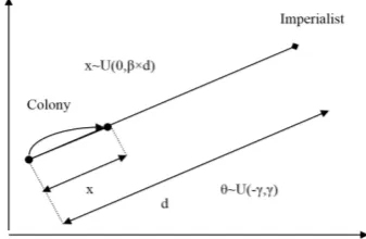
Figure 1: The movement of colonies toward the colonialist.

the colony. x is a uniformly distributed random number defined in equation (4.4) where β is a number greater than one and close to two.

x∼U(0, β×d) (4.4)

A good choice would beβ = 2. Also, the angle of movement is considered as uniform distribution in equation (4.5).

θ∼U(−γ, γ) (4.5)

With a possible deviation in imperialist competi-tive algorithm, the colony moves toward the path of assimilation by the colonialist. This deviation angle is shown by θ that θ is chosen randomly with uniform distribution. During the movement of colonies toward the colonialist country, some of these colonies may reach to a better situation than the colonialist. In this case, the colonial-ist and the colony change their positions with each other. For modeling this competition, given the total cost of empire, first the probability of takeover of colonies by each empire is calculated as equation (4.6).

N.T.C.n=T.C.n−max{T.C.i} (4.6)

where T.C.n is the total cost of the nth empire and N.T.C.n is the total normalized cost of that empire and the possible takeover of the colony by the empire is calculated as equation (4.7) [19].

Ppn =|

N.T.C.n

∑Nimp

i=1 N.T.C.i

| (4.7)

5

Data envelopment analysis

Efficiency measurement because of its impor-tance in assessing the performance of a company

or organization has always been of researcher’s interest. Using a method like the efficiency mea-surement methods in engineering topics, Farrell measured the efficiency of a manufacturing unit in 1975 [5]. The case that Farrell used for the mea-surement of efficiency included an input and an output. Farrell used his model to estimate the ef-ficiency of the U.S. Agricultural Sector compared to other countries. However, he was not suc-cessful in presenting a method that incorporated multiple inputs and outputs. Charnes, Cooper and Rhodes developed the Farrell’s viewpoint and presented a model that was able to measure the efficiency with multiple inputs and multiple out-puts [29]. In their viewpoints, the efficiency of each decision making unit is equal to the ratio of total weighted outputs to total weighted in-puts. In this expression, Ek is the efficiency of

kth_{unit under investigation. y}

rkis the amount of

rthoutput for kthdecision making unit andxik is the amount ofith output forkth decision making unit. ur is the weight of rth output. vi is the weight of ith output. sis the number of outputs and m is the number of inputs of decision mak-ing units. Charnes, Cooper and Rhodes used this measuring technique of efficiency to present a new model. The purpose of the model was measuring and comparing the relative efficiency of organi-zational units with multiple similar inputs and outputs.

Ek=

∑s

r=1uryrk

∑m i=1vixik

(5.8)

unique model must be solved for each unit.

M ax Ek =

∑s

r=1uryrk

∑m i=1vixik

subject to:

∑s

r=1uryrk

∑m i=1vixik

, k= 1, . . . , n,

ur≥0, r= 1, . . . , s,

vi ≥0, i= 1, . . . , m. (5.9)

One of the features of data envelopment analy-sis model is its returns to scale structure. Re-turns to scale can be constant or variable. Con-stant returns to scale means that an increase in input amount leads to proportional increase in the amount of output. In variable returns, the in-crease in output is more or less than the inin-creases ratio in the input. CCR models are among the models with constant returns to scale. Constant returns to scale models are useful when all units operate at an optimal scale. While evaluating the efficiency of the units, if incomplete conditions and space of competition impose restrictions on investment, it leads to inactivity of the unit in optimal scale [23]. In 1984, Banker, Charnes and Cooper made some changes in the CCR model to present a new model called BCC. This model is of data envelopment analysis models types that assesses the relative efficiency of units with vari-able returns to scale [31]. Models with constant returns to scale are more limiting than

M ax E0 =

∑s

r=1ur.yr0+u0

subject to:

∑m

i=1vi.xi0= 1,

∑s

r=1ur.yrk−

∑m

i=1vi.xik+u0 ≤0,∀k, ur, vi≥0, r= 1, . . . , s, i= 1, ..., m. W is free.

(5.10) In model (5.10),xij and yrj represent the jth in-puts and outin-puts of decision making units and

vi and ur are the weights of inputs and outputs. Therefore, in the above model xi0 and yrj are

DM U0 inputs and outputs. Also the sign of u0

can determine returns to scale for each unit.

6

A Framework for the

Cre-ation of a Portfolio of Stocks

with

Hybrid

DEA-BCC

Based CHAID and

Imperial-ist Competitive Algorithm

This part of the paper presents a comprehen-sive and new framework for the creation of stock portfolio based on data mining approach and mul-tiple criteria decision analysis. As observed in Figure 2, in this approach, first the stocks in the stock exchange are classified using CHAID algo-rithm, then each class is ranked by DEA-BCC and hence the initial portfolio is formed. The fi-nal portfolio is obtained by designing a binary two objective mathematical programming model that minimizes the stock risks and maximizes the rank of each share. The Pareto solution of the related mathematical model was obtained through impe-rialist competitive algorithm. The framework

Figure 2: The framework for selection of stocks portfolio.

Figure 4: Taguchi ratio of the first objective func-tion for small-scale problems (20 to 40 variables).

Figure 5: Taguchi ratio of the Second objective function for small-scale problems (20 to 40 vari-ables).

depicted in Figure 2 contains the main following steps;

• Classification: At this stage, the candidate stocks are classified based on the risks labels.

• Ranking: At this stage, it is ranked through DEA-BCC mathematical program-ming model.

• Designing multi-objective binary pro-gramming model: At this stage, a multi-objective binary programming model is de-signed that minimizes the risks per share and maximizes the ranking of each share. Vari-ables and parameters of this model are sum-marized in Table1.

In Table 4, the Beta risk coefficient per share, price per share and the expected return are pre-sented.

Therefore, the two-objective binary mathemat-ical programming model of this paper is presented

Figure 6: Taguchi ratio of the first objective func-tion for large-scale problems (80 to 100 variables).

Figure 7: Taguchi ratio of the second objective function for large-scale problems (80 to 100 vari-ables)

as follows;

M ax z1=

n

∑

i=1

m

∑

j=1

RankDEA−bcciXj

M ax z2=

n

∑

i=1

m

∑

j=1 βiXj,

subject to: n

∑

i=1

m

∑

j=1

ROEiXj ≥R,

n

∑

i=1

m

∑

j=1

ViXj ≤B,

m

∑

j=1

Xj = 1

m

∑

j=1

Xj = 0

Xj ∈ {0,1}

(6.11)

vari-Table 1: Variables and parameters of the mathematical model of stocks portfolio selection.

variables and parameters of the model Description

Xj Binary variablej= 1, ..., m If the Stock j is selected, it is equal to 1, otherwise, it is 0.

βi Risk theithStock

RankDEA−bcci Efficiency obtained from DEA-BCC for thei

th _Stock

R Short term return rate Value

ROEi Return On Equity theithStock

Vi value theithStock

B Budget Capacity

Research objectives;

M ax z1= ∑n

i=1 ∑m

j=1RankDEA−bcciXj 1-maximizing the rank of each portfolio

M ax z2= ∑n

i=1 ∑m

j=1βiXj 2-minimizing the risk of each portfolio Constraints;

∑n i=1

∑m

j=1ROEiXj≥R 1. Return On Equity Constraint

∑n i=1

∑m

j=1ViXj ≤B 2. Budget Constraint

∑m

j=1Xj = 1 3. Mutually Exclusive Stocks Constraint

∑m

j=1Xj = 0 4. Dependent Stocks Constraint

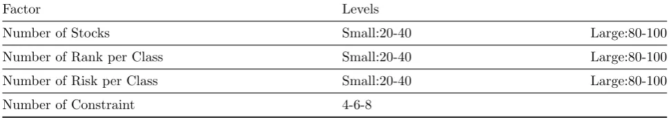
Table 2: Factors studied in stock selection problem by the problem scale.

Factor Levels

Number of Stocks Small:20-40 Large:80-100

Number of Rank per Class Small:20-40 Large:80-100

Number of Risk per Class Small:20-40 Large:80-100

Number of Constraint 4-6-8

ables and large scale problems with 80-100 vari-ables. However, in the case study section, input data is displayed only for 20 variables. The prob-lem constraints also respectively increased to 4, 6 and 8. Thus Model 11 is studied in small and large-scales. Table 2shows the described factors:

• Optimization: At this stage, the Pareto so-lution of the model 11 with multi objective algorithm is analyzed using the imperialist competitive algorithm.

7

Case Study

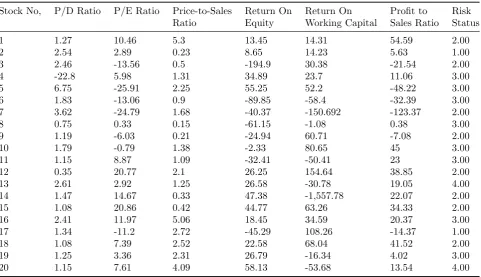
Table 3: The study input data.

Stock No, P/D Ratio P/E Ratio Price-to-Sales Return On Return On Profit to Risk Ratio Equity Working Capital Sales Ratio Status

1 1.27 10.46 5.3 13.45 14.31 54.59 2.00

2 2.54 2.89 0.23 8.65 14.23 5.63 1.00

3 2.46 -13.56 0.5 -194.9 30.38 -21.54 2.00

4 -22.8 5.98 1.31 34.89 23.7 11.06 3.00

5 6.75 -25.91 2.25 55.25 52.2 -48.22 3.00

6 1.83 -13.06 0.9 -89.85 -58.4 -32.39 3.00

7 3.62 -24.79 1.68 -40.37 -150.692 -123.37 2.00

8 0.75 0.33 0.15 -61.15 -1.08 0.38 3.00

9 1.19 -6.03 0.21 -24.94 60.71 -7.08 2.00

10 1.79 -0.79 1.38 -2.33 80.65 45 3.00

11 1.15 8.87 1.09 -32.41 -50.41 23 3.00

12 0.35 20.77 2.1 26.25 154.64 38.85 2.00

13 2.61 2.92 1.25 26.58 -30.78 19.05 4.00

14 1.47 14.67 0.33 47.38 -1,557.78 22.07 2.00

15 1.08 20.86 0.42 44.77 63.26 34.33 2.00

16 2.41 11.97 5.06 18.45 34.59 20.37 3.00

17 1.34 -11.2 2.72 -45.29 108.26 -14.37 1.00

18 1.08 7.39 2.52 22.58 68.04 41.52 2.00

19 1.25 3.36 2.31 26.79 -16.34 4.02 3.00

20 1.15 7.61 4.09 58.13 -53.68 13.54 4.00

Table 4: Beta risk coefficient per share, price per share and the expected return.

stock 1 2 3 4 5 6 7 8 9 10

risk 0.2 0.8 0.6 0.9 0.4 0.5 0.3 0.8 0.4 0.3

price 1 1.5 1.2 1.8 1.1 1.4 1.3 1.4 1.6 1.8

return 0.2 0.15 0.23 0.22 0.21 0.14 0.2 0.22 0.24 0.21

stock 11 12 13 14 15 16 17 18 19 20

risk 0.1 0.4 0.7 0.6 0.8 0.4 0.3 0.7 0.3 0.7

price 1.6 1.5 1.2 1.4 1.2 1.3 1.9 1.3 1.4 1.5

return 0.23 0.24 0.21 0.25 0.22 0.2 0.19 0.18 0.17 0.22

The last column of Table3is associated with the risk status that range from very low value (1) to low value (2), high value (3) and very high value (4). This scale is an Ordinal Measure.

Meanwhile, the total budget of institute is 15.6. It is expected that the dividends reach 2.3 mon-etary units for the total investment. After run-ning the CHAID algorithm with IBM Modeler 14.2 software, the decision rules were derived as follows; Rule 1: If Return on working cap-ital > −1.078 and Return on working capital

≤14.312 then Risk is 1.

Rule 2: If Return on working capital > 80.648 then risk is 1.

Rule 3: If Return on working capital≤ −150.692 then risk is 2.

Rule 4: If Return on working capital > 14.312 and Return on working capital ≤ 80.648 then Risk is 2.

Table 5: Positive values of the input data.

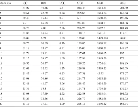
Stock No I(1) I(2) O(1) O(2) O(3) O(4)

1 31.27 40.46 5.3 213.45 1614.31 204.59

2 32.54 32.89 0.23 208.65 1614.23 155.63

3 32.46 16.44 0.5 5.1 1630.38 128.46

4 7.2 35.98 1.31 234.89 1623.7 161.06

5 36.75 4.09 2.25 255.25 1652.2 101.78

6 31.83 16.94 0.9 110.15 1541.6 117.61

7 33.62 5.21 1.68 159.63 1449.308 26.63

8 30.75 30.33 0.15 138.85 1598.92 150.38

9 31.19 23.97 0.21 175.06 1660.71 142.92

10 31.79 29.21 1.38 197.67 1680.65 195

11 31.15 38.87 1.09 167.59 1549.59 173

12 30.35 50.77 2.1 226.25 1754.64 188.85

13 32.61 32.92 1.25 226.58 1569.22 169.05

14 31.47 44.67 0.33 247.38 42.22 172.07

15 31.08 50.86 0.42 244.77 1663.26 184.33

16 32.41 41.97 5.06 218.45 1634.59 170.37

17 31.34 18.8 2.72 154.71 1708.26 135.63

18 31.08 37.39 2.52 222.58 1668.04 191.52

19 31.25 33.36 2.31 226.79 1583.66 154.02

20 31.15 37.61 4.09 258.13 1546.32 163.54

Table 6: Beta risk coefficient per share, price per share and the expected return.

Stock 1 2 3 4 5 6 7 8 9 10

Class 1 1 4 4 4 5 3 5 4 2

Efficiency 1 0.99 0.95 1 1 1 1 1 1 1

Stock 11 12 13 14 15 16 17 18 19 20

Class 5 2 5 3 4 4 2 4 5 5

Efficiency 1 1 1 1 1 1 1 1 1 1

As specified in the decision rules, the number of classes relating to the research data is equal to 5 classes. The stocks 1 and 2 fall in the first class, the stocks 10, 17 and 12 fall in the second class, the stocks 14 and 7 fall in the third class, the

transforma-Table 7: The main settings for application of ICA Algorithm.

Parameters Value

Number of Imperialist 10

Number of Population 200

Max of Decades 700

Beta 0.4

Table 8: Average Pareto combination of risk and rank.

Solution 1 2 3 4 5 6 7 8 9 10

Rank -2.001 -2 -2 -1.001 -1 -1 -1 -1 -1 -0.99

Risk 1.301 1.1 0.8 0.901 0.8 0.7 0.6 0.4 0.3 0.2

Table 9: Types of Taguchi functions for calibration.

Performance S/N ratio formula Description of formula parameters

characteristic/metric

Smaller the better S/N=−10log[_n1∑n_i=1OF_i2] n=number of observation (signals) OF=Objective Function

Nominal is best Mean and Variance, OF=Average of Observation of Objective Function, S/N=−10log(S2) Variance only, S=Standard Deviation of n observation

S/N= 10log(OF_S¯ )2

Larger the better S/N=−10log[_n1∑n_i=1OF12 i

] n=number of observation (signals) OF=Objective Function

Table 10: Settings for sensitivity analysis of the model with Taguchi method for small-scale problems.

Factors Value

Zeta 0.5-0.6

Revolution Rate 0.1-0.2

Number of Imperialist 10-20

Number of (Countries-Iteration) (200,700)-(300-1000)

tion result is provided in Table5.

Based on the translation invariant concept in Table 5, +30 was added to the first input ues, +30 was also added to the second input ues, +200 was added to the second output val-ues, +1600 was added to the third output values and +150 was added to the fourth output values.

The first phase of the input oriented DEA-BCC model for the sixth unit which is located in the fifth class is shown in 12. It should be noted that in this study, P/E and P/D were input criteria and other parameters were considered as output criteria.

M in y0 =θ,

Table 11: Settings for sensitivity analysis of the model with Taguchi method for large-scale problems.

Factors Value

Zeta 0.5-0.6

Revolution Rate 0.1-0.2

Number of Imperialist 10-20

Number of (Countries-Iteration) (400,1000)-(500-1200)

1.83λ1+ 0.75λ2+ 1.15λ3

+2.61λ4+ 1.25λ5+ 1.15λ6≥1.83,

−13.06λ1+ 0.33λ2+ 8.87λ3+ 2.92λ4

+3.36λ5+ 7.61λ6 ≥ −13.06,

−0.90θ+ 0.90λ1+ 0.15λ2+ 1.09λ3

+1.25λ4+ 2.31λ5+ 4.09λ6 ≤0,

89.85θ−89.85λ1−61.15λ2−32.41λ3

+26.58λ4+ 26.79λ5+ 58.13λ6 ≤0,

58.40θ−58.40λ1−1.08λ2−50.41λ3

−30.75λ4−16.34λ5−53.68λ6 ≤0,

32.39θ−32.39λ1+ 0.38λ2+ 23λ3

+19.05λ4+ 4.02λ5+ 13.54λ6 ≤0,

λ1+λ2+λ3+λ4+λ5+λ6 = 1,

λj ≥0, θis free.

The second phase of DEA-BCC input oriented arrayed model is presented in model 12 with de-scription 13:

M ax S=s+₁ +s+₂ +s₃++s+₄ +s−₁ +s−₂

S.t:

(7.13) 1.83λ1+ 0.75λ2+ 1.15λ3+ 2.61λ4

+1.25λ5+ 1.15λ6−s−₁ = 1.83,

−13.06λ1+ 0.33λ2+ 8.87λ3+ 2.92λ4

+3.36λ5+ 7.61λ6−s−2 =−13.06,

−0.90θ∗+ 0.90λ1+ 0.15λ2+ 1.09λ3

+1.25λ4+ 2.31λ5+ 4.09λ6+s+1 = 0,

89.85θ∗−89.85λ1−61.15λ2−32.41λ3

+26.58λ4+ 26.79λ5+ 58.13λ6+s+₂ = 0,

58.40θ∗−58.40λ1−1.08λ2−50.41λ3

−30.75λ4−16.34λ5−53.68λ6+s+3 = 0,

32.39θ∗−32.39λ1+ 0.38λ2+ 23λ3

+19.05λ4+ 4.02λ5+ 13.54λ6+s+4 = 0,

λ1+λ2+λ3+λ4+λ5+λ6 = 1,

λj ≥0, s+₁ ≥0, s+₂ ≥0, s+₃ ≥0,

s+₄ ≥0, s−₁ ≥0, s−₂ ≥0.

Table6shows the efficiency of candidate locations in each cluster using input oriented DEA-BCC model.

For implementation of Imperialist Competitive algorithm, 30 independent tests are used. Aver-age solution for the small scale problem with 20 variables can be seen in Table 8 and Figure3.

Based on the model presented in this study, the binary two objective programming model is structured as follows:

M ax Z1 =x1+ 0.99x2+ 0.95x3+x4

+x5+x6+x7+x8+x9+x10

+x11+x12+x13+x14+x15

+x16+x17+x18+x19+x20,

(7.14)

M in Z2 = 0.2x1+ 0.8x2+ 0.6x3+ 0.9x4

+0.4x5+ 0.5x6+ 0.3x7+ 0.8x8

+0.4x9+ 0.3x10+ 0.1x11+ 0.4x12

+0.7x13+ 0.6x14+ 0.8x15+ 0.4x16

+0.3x17+ 0.7x18+ 0.3x19+ 0.7x20

s.t:

1x1+ 1.5x2+ 1.2x3+ 1.8x4+ 1.1x5

+1.4x6+ 1.3x7+ 1.4x8+ 1.6x9

+1.4x14+ 1.2x15+ 1.3x16+ 1.9x17

+1.3x18+ 1.4x19+ 1.5x20≤15.6,

0.2x1+ 0.15x2+ 0.23x3+ 0.22x4

+0.21x5+ 0.14x6+ 0.2x7+ 0.22x8

+0.24x9+ 0.21x10+ 0.23x11+ 0.24x12

+0.21x13+ 0.25x14+ 0.22x15+ 0.2x16

+0.19x17+ 0.18x18+ 0.17x19

+0.22x20≤2.3,

x11+x16≤1,

x4−x8 ≤0,

xi∈ {0,1}, i= 1,2, ...,20.

The result of application of binary two ob-jective imperialist competitive algorithm can be seen in figure 3. In order to conduct the exper-iments, we implemented imperialist competitive algorithm in MATLAB R2010a run on a personal computer with a 2.3GHz up to 2.8 GHz Core i5 and 2 GB RAM memory. The main parameters of algorithm are summarized in Table 7.

8

Sensitivity Analysis

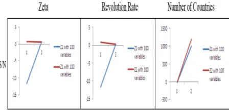
The Taguchi method is used to analyze the model sensitivity. The model control parameters are cal-ibrated through the Taguchi Method. The ba-sis for calibrating the control parameters in the Taguchi method is the signal to noise ratio. The term signal refers to the values of desired vari-ables and the term noise refers to the values of unfavorable variables. The S/N ratio refers to the variance in response to the variable.According to the type of objective function, one of the func-tions in Table 9 is used for analysis of control parameters: Zeta, Revolution Rate and Number of Countries.

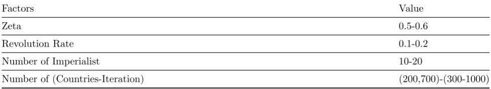
To analyze the results with the Taguchi method with small scale problems, the studied model el-ements are defined as seen in Table 10. Results for the first and second objective functions can be seen in figures 4 and5.

As can be seen in figures 4 and5, the problem is calibrated in small scale based on the Taguchi method. To analyze the results with Taguchi

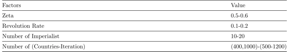
method with the large scale problems, the stud-ied model elements are defined as seen in Table 11.

Results for the first and second objective func-tions can be seen in figures 6 and 7.

As can be seen, the problem is calibrated in large scale based on the Taguchi method.

9

Conclusion

One of the most important issues for investors in stock exchange markets is the stocks selection technique. Achieving the methods that can as-sist investors in selecting stocks in the stock ex-change is very important. If investors act ratio-nally in stock selection decisions, they can achieve the desired return. The important factor that can help investors to select the optimal stocks is concentration on the criteria approved by finan-cial experts and spefinan-cialists. The important point in the stock investment is that decision making is not a one dimensional process. The success-ful decision maker is the one who decides the is-sue from different aspects and jointly and simul-taneously uses multiple criteria and then, while investigating different factors influencing on that choice, selects the best options based on their pri-orities. In order to select a portfolio of Stocks through CHAID data mining algorithm in this paper, first the studied stocks were classified. The classified stocks were ranked using the DEA-BCC model. Through a binary two objective program-ming model, the combination of risk and rating Pareto was analyzed based on imperialist com-petitive algorithm.

References

[1] E. Atashpaz-Gargari, C. Lucas, Imperialist competitive algorithm: an algorithm for op-timization inspired by imperialistic competi-tion,In 2007 IEEE congress on evolutionary computation 4 (2007) 4661-4667.

[3] R. Castellano, R. Cerqueti, Mean Variance portfolio selection in presence of infrequently traded stocks, European Journal of Opera-tional Research 234 (2014) 442-449.

[4] C. C¸ iflikli, E. Kahya- ¨Ozyirmidokuz, Im-plementing a data mining solution for en-hancing carpet manufacturing productivity,

Knowledge-Based Systems 23 (2010) 783-788.

[5] W. W. Cooper, Data envelopment analy-sis,Encyclopedia of Operations Research and Management Science (2001) 183-191. [6] K. Deb, Multi-objective optimization

us-ing evolutionary algorithms, John Wiley & Sons, 2001.

[7] R. Eberhart, J. Kennedy, A new optimizer using particle swarm theory,InMHS’95. Pro-ceedings of the Sixth International Sympo-sium on Micro Machine and Human Science

6 (1995) 39-43.

[8] A. T. Eshlaghy, F. F. Razi, A hybrid grey-based KOHONEN and genetic algorithm to integrated technology selection, Interna-tional Journal of Industrial and Systems En-gineering 20 (2015) 323-342.

[9] F. Faezy Razi, A. T. Eshlaghy, J. Nazemi, M. Alborzi, A. Pourebrahimi, A hybrid grey based KOHONEN model and biogeography-based optimization for project portfolio se-lection, Journal of Applied Mathematics

(2014).

[10] K. Gnanendran, J. K. Ho, R. P. Sundarraj, Stock selection heuristics for interdependent items, European Journal of Operational Re-search 145 (2003) 585-605.

[11] F. Gorunescu, Data Mining: Concepts, mod-els and techniques,Springer Science & Busi-ness Media, 2011.

[12] J. Han, J. Pei, M. Kamber, Data mining: concepts and techniques, Elsevier, 2011. [13] J. H. Holland, Adaptation in natural and

artificial systems: an introductory analysis with applications to biology, control, and ar-tificial intelligence,MIT press, 1992.

[14] H. C. Huang, T. K. Lin, P. W. Ngui, Analysing a mental health survey by chi-squared automatic interaction detection,

Annals of The Academy of Medicine, Sin-gapore 22 (1993) 332-337.

[15] K. Y. Huang, C.-J. Jane, A hybrid model for stock market forecasting and portfolio se-lection based on ARX, grey system and RS theories,Expert systems with applications 36 (2009) 5387-5392.

[16] S. Hwang, J. Park, Performance Evaluation with Information on Portfolio Compositions,

AsiaPacific Journal of Financial Studies 40 (2011) 710-730.

[17] A. Ishizaka, P. Nemery, Assigning machines to incomparable maintenance strategies with ELECTRE-SORT,Omega 47 (2014) 45-59. [18] M. Kantardzic, Data mining: concepts,

models, methods, and algorithms,John Wi-ley & Sons, 2011.

[19] A. Kaveh, Advances in metaheuristic al-gorithms for optimal design of structures,

Springer, 2014.

[20] S. Kirkpatrick, C. D. Gelatt, M. P. Vecchi, Optimization by simulated annealing, sci-ence 220 (1983) 671-680.

[21] R. K. Lai, C.-Y. Fan, W.-H. Huang,P.-C. Chang, Evolving and clustering fuzzy deci-sion tree for financial time series data fore-casting,Expert Systems with Applications 36 (2009) 3761-3773.

[22] D. T. Larose, C. D. Larose, Discovering knowledge in data: an introduction to data mining,John Wiley & Sons, 2014.

[23] C. A. K. Lovell, J. T. Pastor, Units invariant and translation invariant DEA models, Op-erations research letters 18 (1995) 147-151. [24] D. Maringer, Portfolio management with

heuristic optimization,Springer, 2005. [25] J. A. McCarty, M. Hastak, Segmentation

[26] D. L. Olson, D. Delen, Advanced data min-ing techniques, Springer Science, Business Media, 2008.

[27] J.-L. Prigent, Portfolio optimization and performance analysis,CRC Press, 2007. [28] R. V. Rao, Decision making in the

manu-facturing environment: using graph theory and fuzzy multiple attribute decision mak-ing methods, Springer Science & Business Media, 2007.

[29] S. C. Ray, Data Envelopment Analysis: The-ory and Techniques for Economics and Oper-ations Research,Cambridge university press, 2004.

[30] F. F. Razi, A. T. Eshlaghy, J. Nazemi, M. Alborzi, A. Poorebrahimi, A hybrid grey-based fuzzy C-means and multiple objective genetic algorithms for project portfolio selec-tion,International Journal of Industrial and Systems Engineering 21 (2015) 154-179. [31] L. M. Seiford, J. Zhu, Modeling

undesir-able factors in efficiency evaluation, Euro-pean Journal of Operational Research 142 (2002) 16-20.

[32] J. Shadbolt, J. G. Taylor, Neural Net-works and the Financial Markets: Bpredict-ing, CombinBpredict-ing, and Portfolio Optimisation,

Springer, 2002.

[33] K.-Y. Shen, M.-R. Yan, G.-H. Tzeng, Com-bining VIKOR-DANP model for glamor stock selection and stock performance im-provement, Knowledge-Based Systems 58 (2014) 86-97.

[34] F. Tiryaki, B. Ahlatcioglu, Fuzzy portfolio selection using fuzzy analytic hierarchy pro-cess,Information Sciences 179 (2009) 53-69. [35] F. Tiryaki, M. Ahlatcioglu, Fuzzy stock selection using a new fuzzy ranking and weighting algorithm, Applied Mathematics and Computation 170 (2005) 144-157. [36] M. van Diepen, P. H. Franses, Evaluating

chi-squared automatic interaction detection,

Information Systems 31 (2006) 814-831.

[37] M. C. Wong, Y. L. Cheung, The prac-tice of investment management in Hong Kong: market forecasting and stock selec-tion,Omega 27 (1999) 451-465.

[38] P. Xidonas, G. Mavrotas, T. Krintas, J. Psarras, C. Zopounidis, Multicriteria port-folio management,Springer, 2012.

[39] B. Xing, W.-J. Gao, Introduction to Compu-tational Intelligence, In Innovative Compu-tational Intelligence: A Rough Guide to 134 Clever Algorithms 5 (2014) 3-17. Springer, Cham.

[40] H. Yu, R. Chen, G. Zhang, A SVM stock selection model within PCA, Procedia com-puter science 31 (2014) 406-412.

[41] X. Zhang, Y. Hu, K. Xie, S. Wang, E. W. T. Ngai, M. Liu, A causal feature selection al-gorithm for stock prediction modeling, Neu-rocomputing 142 (2014) 48-59.