A Study of Flow and Mixing in Bubbly Gas-Liquid Pipe Flow Generated by a Grid

(1)

60

Iranian Journal of Chemical Engineering Vol. 3, No. 4 (Autumn), 2006, IAChE

A Study of Flow and Mixing in Bubbly Gas-Liquid

Pipe Flow Generated by a Grid

J. S. Moghaddas1∗, C. Trägårdh2, J. Revstedt3, K. Östergren2

1- Chemical Engineering Faculty, Sahand University of Technology, P.O. Box 51335/1996, Tabriz, I.R. IRAN.

(2,3) Lund Institute of Technology at Lund University.

2- Division of Food Engineering, P.O. Box 124, SE-221 00 Lund, Sweden. 3- Division of Fluid Mechanics, P.O. Box 118, SE-221 00 Lund, Sweden.

Abstract

The spreading of a tracer in a bubbly two-phase grid-generated turbulent flow system is studied. In this work both particle image velocimetry (PIV) and planer laser-induced fluorescence (PLIF) are used to study the effect of the dispersed phase flow rate on the mixing characteristics of the tracer. The turbulent intensity of the continuous phase in the bubbly two-phase grid-generated turbulent flow is close to isotropic, and increasing the gas void fraction reduces the degree of non-isotropicity. The self-similarity of mean and RMS values of the cross-stream concentration distribution is observed. A new mathematical model is suggested to describe the self-similarity of the cross-stream profiles of the mean concentration based on two separate Gaussian curves into the central and outer region of the flow. The turbulent diffusivity is calculated using the Taylor hypothesis, which is based on the growth of the variance of the cross-stream profiles of the mean concentration, with a position along the direction of the flow. An increase in the void fraction does not affect the diffusivity of the superimposed distribution of the plume in the central region, however it did increase in the outer region.

Keywords: Grid-generated turbulence, mixing, PIV, PLIF, diffusivity

∗ - Corresponding author: E-mail: [email protected]

Introduction

Some processes in the biotechnical, chemical and food industries which employ turbulent bubbly gas-liquid flow systems designed to mass transfer duties also enforce the mixing phenomena in the liquid phase. Turbulence affects the rate of mass transfer, controls dispersion within the flow field, and may also be responsible for flow regime

(2)

two-Iranian Journal of Chemical Engineering, Vol. 3, No. 4 61

phase flow. The bubble and bubble-liquid interactions in turbulent flow can make extremely random motions for gas and liquid phases. These random motions are reflected in the turbulent intensity and diffusivity of the liquid phase.

Many researchers have studied the effects of bubbles on the turbulence in bubbly two-phase flows. Akimi Serizawa et al. [1] developed an electronic instrument for determining various important local para-meters in a bubbly two-phase pipe flow such as the velocity of the bubbles and water, turbulent intensity, and the turbulent dis-persion coefficient of the bubbles. Their experimental results showed that most local parameters are uniformly distributed in the cross-stream direction over most of the cross section in the fully developed bubbly region. On the other hand, it was found that the maximum effect of the local void fraction was near the wall, and a higher turbulent intensity towards the wall and a minimum at the centre of the pipe was predicted. For the constant water flow rate, experimental results indicated a trend for the streamwise turbulent intensity to decrease with the increa-sing gas flow rate, and then increase with a further increase in the gas flow rate [1].

The laser velocimetry technique has been used for turbulence measurements in bubbly two phase pipe flow. Significant departures for mean velocity profiles and higher values of void fraction and relative intensity near the wall have also been observed. Beyerlein et al. [2] presented a model that predicts a wall-skewed bubble distribution by incorporating into the equation of motion of a lateral force due to the relative velocity of the two phases and the eddy diffusivity of the liquid. They mentioned that with an increase in void fraction, the importance of the lateral force would be expected to decrease owing to the interaction between the bubbles. They also believed that cross-stream bubble migration in turbulent flow is claimed to be a product of a circulation-induced lateral force

and bubble diffusion. The former is due to interplay between buoyancy and the fluid velocity gradient, while the latter is actuated by the turbulence in flow.

Recently, some researchers have determined the local properties of both phases in bubbly two-phase flow [3-5]. The variety of methods used and the results obtained show that the exact determination of the local parameters of two-phase flow is very difficult, nonethe-less, recent research has led to a better understanding of bubbly two-phase flow. A few researchers have studied bubbly, two-phase, grid-generated turbulent flow. For example, Lance & Batailie [6] performed studies on the turbulence of the liquid in a bubbly, grid-generated turbulent flow field. They found distinctly different flow behaveiour for lower (dilute) and higher (dense) void fractions of the dispersed phase. For dilute two-phase flow hydrodynamics, interactions between bubbles were negli-gible, but in the dense flow regime the bubbles transferred a greater amount of kinetic energy to the liquid. Panidis & Papailiou [7] studied the influence of the gas bubbles on the structure of turbulence flow downstream of a grid in a rectangular channel. Their observations showed nearly flat distribution of the streamwise turbulent

intensity component, TIx, in the central

region of the channel for low values of the gas flow rate. However, significant redistribution of the void in the channel was observed, resulting in the development of void and velocity peaks between the centre of the channel and the wall.

(3)

62 Iranian Journal of Chemical Engineering, Vol. 3, No. 4

various refinements have recently been developed such as PIV with fluorescent particle tracers, PIV/shadowmetry and PIV/PLIF. In this study the PLIF and PIV measurement techniques are used for concentration and velocity measurements, respectively.

Studies characterising the dispersion of a liquid-tracer plume injected into bubbly two-phase flow are lacking. Hence, the mixing at a grid-generated turbulent flow in the case of the bubbly two-phase flow, and the effects of bubbles were, therefore, the subject of this study. In the present experiments, a water solution of a tracer is injected through a nozzle into the centre of the pipe with the same velocity as the main liquid flow in order to avoid strong shear layers between the two streams.

Materials and methods

In this study two series of measurements on concentration (PLIF) and velocity (PIV) were performed, separately. The same flow conditions, such as liquid and air gas flow rates, were used for both PLIF and PIV measurements.

Flow and optical facilities

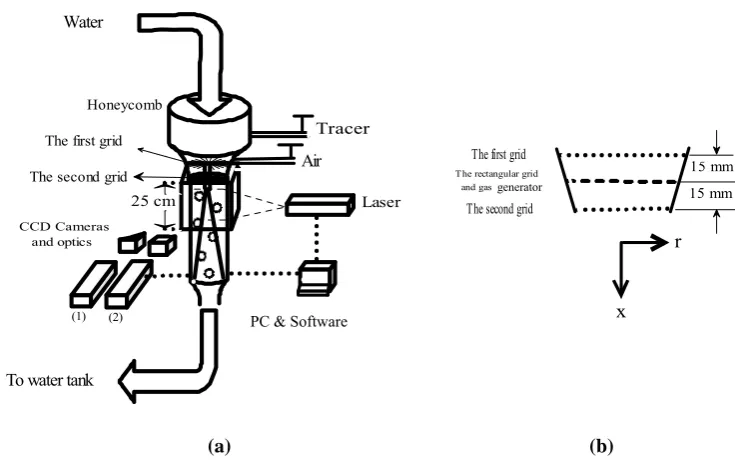
Figure 1a shows a schematic diagram of the experimental set-up and the optical arrange-ment. In concentration measurements using PLIF, the main part of the continuous phase flow is the water solution of the well-mixed reference tracer, LDS-722 (Exciton, Inc., Dayton, Ohio, USA). The solution is pumped into the flow system at a constant concentration from a large stainless steel tank. A frequency meter, controlling the rotational speed of the pump shaft, 3 pressure gauges and a flow meter control the flow rate.

The test section is a glass pipe (DURAN®_,

refractive index 1.47 at 587 nm), with a 75-mm inner diameter, which is positioned vertically. A honeycomb, two circular grids with a 2-mm mesh size, a rectangular grid with a 6-mm mesh size, and the contraction

between the grids are the main components that produce the turbulence before the test section.

To reduce the effects of the rectangular grid, the gas injector (regarding the homogeneity of the turbulence, a second circular grid with the same mesh size as the first grid) is placed at the entrance of the test section. The arrangement of the two circular grids and the rectangular grid, which is the bubble-generator grid, is shown in Figure 1b. Hence, the rectangular grid is placed midway between the circular grids. With this arrangement, the second circular grid has the greatest effect on the main turbulence in the vertical test section.

A stainless steel injector (1.3-mm inner and 1.6-mm outer diameters) injects the second tracer, Rhodamine-6G (Exciton, Inc., Dayton, Ohio, USA) solution. A sensitive medical pump with an easily controllable flow rate pumps this solution as a plume into the centre of the main flow. The liquid continuous-phase is a combination of two-tracer solutions, Rhodamine and the reference tracer LDS. The exit of the Rhodamine injector is positioned 52 mm downstream of the second grid.

Air is uniformly injected into the liquid flow by passing it through 190 holes with a 0.7 mm inner diameter, located on a rectangular grid (6 mm mesh size and 2 mm in bar size). The outlet angle of each hole to the flow direction is _{45 , which reduces the}D

production of eddies by the rectangular grid. To study the effect of the gas volume void fraction on the mixing characteristics, two different gas flow rates, ₃_.₄₈_×₁₀−5_and

5

10 37 .

6 × − m3/s, with the same water flow

(4)

Iranian Journal of Chemical Engineering, Vol. 3, No. 4 63

25 cm Laser

PC & saftware

(1) (2)

CCD Cameras and optics

Honeycomb

The second grid The first grid

x r Air

Tracer Water

To water tank

The first grid

The second grid

The rectangular grid and gas genarator

15 mm 15 mm

(a) (b)

Figure 1. a) A schematic of the set-up. b) The arrangement of grids at the entrance of the test section.

To calculate the void fraction of the dispersed phase the ratio of the volumetric flow rates of air and water were used. Using two pressure gauges, the pressure of air near the gas flow meter and inside the flow is measured. By applying Boyle-Mariotte’s law, P₁V₁ =P₂V₂, for air at room temperature and low pressures (very close to the atmospheric pressure) the gas flow rates were calculated inside the two-phase flow system. Visual inspection revealed the bubbles occupied around 70% of the cross-sectional area of the flow channel, as there was a wall region almost free from bubbles. The average

void fraction in the measured volume (α)

was 1.3% for an air flow rate of ₃_.₄₈_×₁₀−5

m3/s and 2.4% for the higher rate of

5

10 37 .

6 × − m3/s.

The light sheet was generated using a

double-cavity 2×25 mJ Nd:Yag pulsed laser

at a wavelength of 532 nm. The laser light sheet has a mean thickness of 1 mm. It is passed through a plano-convex lens and directed on to the central part of the pipe. The beam is then passed through the flow system containing the two fluorescent tracers in the liquid phase, which emit in the red and

green region of the wavelength spectrum. The first tracer, LDS, is used as a reference tracer, while the second, Rhodamin-6G, gives a measure of the concentration. Two tracers are used to reduce the optical problems encountered in bubbly two-phase flow. For more information the reader is referred to Moghaddas et al. [8]. In brief, the florescence intensity of the Rhodamin in the bubbly two-phase system is calculated based on the intensity emitted by LDS, which has a constant concentration in both single- and two-phase flow systems.

Two high-resolution (1280×1024 pixels)

CCD cameras (Flow Master), which are mounted side by side on a platform, record the PLIF images of each tracer, separately. The images are transferred to a Pentium-based PC using commercial software (Lavi-sion). Both CCD cameras are adjusted to capture the images of the flow from the same region in the test section. A beam splitter and a mirror are used to split the incoming light between the two CCD cameras.

To record the PLIF signals of LDS the first CCD camera is equipped with two red long-pass filters, RG665 and RG695 (Melles

PC & Software

(5)

Griot), with centre wavelength cut-offs at 665 and 695 nm. The fluorescent light emitted by Rhodamine is detected by the second CCD camera after passing through a band-pass filter centred at 573 nm, with Δλ= 5 nm, and a long-pass filter, OG570 (Melles Griot), with a centre wavelength cut-off at 570 nm. Two filters for each CCD camera were used to ensure that each camera captured the fluorescent signal emitted by only one tracer.

In the case of velocity studies using PIV, the liquid phase consists of only water seeded with Rhodamine-B fluorescent tracer

particles, 1-20 μm in diameter, which are

excitable at the wavelength of the pulsed laser. The continuous liquid phase flow rate was the same as that used in the PLIF measurements. The filters used on the CCD camera are two long-pass filters, OG550 and OG570 nm, which only allow the passage of fluorescent light from the Rodamine particles.

PLIF calibration procedure

At the beginning of the calibration process, both CCD cameras measure the light intensity in both single- and two-phase flow for pure water. These data are used as the background intensities corresponding to the zero concentration of each tracer. Then, in a similar way to the background calibration measurements, data are collected for a constant concentration of the first tracer, LDS, in both single- and two-phase flow. In the case of the two-phase flow, the second CCD camera measures the calibration data for the second tracer, Rhodamine. Throughout the whole calibration procedure the flow rate of the liquid and gas phases were constant. The effects of air bubbles on the fluorescence data, i.e. reflections and shadowing, creating a very non-uniform distribution of light intensity, have been explained previously [9]. These optical effects can be taken into account when evaluating the concentration of the second tracer by making use of the light intensity

data for the reference tracer, obtained at a constant concentration in the liquid phase. According to the Lambert-Beer law, at low concentrations of the tracers, there is a linear relation between the fluorescence intensity emitted and the concentration. The PLIF image data are stored in two-dimensional matrix form, so the linear relation for each pixel could be given as:

= Ω

f ( i , j ) ( i , j ) ( i , j )

I C (1)

where the index “i” indicates the position of

the chosen pixel at the cross stream, and

“ j” the position in the flow (streamwise)

direction. “If” is the fluorescent intensity, “C” is the instantaneous concentration of the tracer, and “Ω” is the calibration coefficient at each pixel. In this study, calibration according to Eq. (1) was performed separately for each pixel in a Matlab program. These data are then used for further calculations.

Figure 2 shows typical calibration curves for 200 pixels in the cross-stream direction for a

chosen streamwise location, =

M x

73, in the

(6)

single- and bubbly two-phase flow. The calculations in both the calibration and the experiments are based on the average of 1000 successive images at each chosen flow rate.

(a)

(b)

Figure 2. Typical calibration curves. a) Gas void

fraction, α =1 3. %. b) Gas void fraction, α =2 4. %.

The mean and RMS values of concentration for the Rhodamine tracer were calculated using the calibration coefficient for every pixel in the 1000 two-dimensional images for both void fractions of gas. The accuracy of the measured data upon changing the number of observations was tested using statistical analysis. When increasing the number of

images to 400 in this experiment, constant values for the four statistical moments were obtained.

Results and discussion

Velocity

In bubbly two-phase flow systems, measuring the correct size of the bubbles is difficult using laser techniques. In this study it was estimated that the bubbles were about two millimetres in diameter by scaling the bubble sizes on several PIV images. This is in good agreement with the values expected from theory [10].

Figure 3 shows the mean values of the velocity of the continuous phase at two positions in the flow direction:

M x

, 73 and

84 for both gas-void fractions. The results show a lower velocity in the central region of the pipe. This may be explained by a variation in the cross-sectional void fraction profile, as was observed by Panidis and Papailiou [7] in a grid set-up. For a lower gas-void fraction, lower velocity is found in the central region at both mentioned positions. The bubbly two-phase hydro-dynamic forces such as drag and lift, and the particular inlet configuration are the reasons for this behaviour. There is also a region, as mentioned above, along the wall where the bubble number density is very low. Therefore, this is a result of processes inherent to the nature of two-phase flow, as well as the design of the particular set-up. Figure 4 shows the values of the velocity in the cross-stream direction at two positions in the flow direction: x/M = 73 and 84. The variation in the cross-stream velocity is about

015 . 0

± m/s, i.e. around 1% of the mean flow

(7)

-30 -20 -10 0 10 20 30

0.6 0.8 1 1.2 1.4

1.6 Liquid-phase velocity profiles in r-direction, x/M = 73.228

r (mm)

U

x (

m

/s

)

o alfa=2.4% x alfa=1.3%

(a)

-30 -20 -10 0 10 20 30

0.6 0.8 1 1.2 1.4

r (mm)

U

x (

m

/s)

o alfa=2.4% x alfa=1.3%

(b)

Figure 3. The measured mean velocity profile of the

continuous phase for both void fractions: α =1 3. % and α =2 4. %. a) x/M = 73 b) x/M = 84.

Assuming an average slip velocity Ux−Vx of ≈0.2m/s, a surface tension between air bubbles and water _γ ₌₇_.₂_×₁₀−2_{N/m [11]}

and an average bubble diameter Db ≈2 mm,

the bubble Reynolds number

ν

b x x b

D V U −

=

Re and the Eötvös number,

γ ρ

ρ 2

b bD

g

Eo= − can be calculated, giving

(a)

(b)

Figure 4. The cross-stream velocity of the continuous

phase at two positions: a) x/M = 73 b) x/M = 84.

values of 400 and 0.544, respectively. In this work, the subscripts x and r represent the

streamwise and cross-stream directions in the flow. Ux and Vx are the mean streamwise velocities, ρ and ρb are the densities of the continuous and dispersed flow, respectively,

and Db is the average diameter of the

bubbles. According to Clift et al. [12], the shape of the bubbles in bubbly two-phase flow can be treated as ellipsoidal. For larger bubbles the Laplace pressure is not sufficient to maintain the spherical shape and the bubbles become slightly ellipsoidal.

Ellip-× α = 1.3%

o α = 2.4 %

× α = 1.3%

o α = 2.4 %

-30 -20 -10 0 10 20 30

-0.03 -0.02 -0.01 0 0.01 0.02 0.03 0.04

r (mm)

U

r (

m

/s

)

o alfa=2.4% x alfa=1.3%× α = 1.3%

o α = 2.4 %

-30 -20 -10 0 10 20 30

-0.03 -0.02 -0.01 0 0.01 0.02 0.03 0.04

r (mm)

U

r (

m

/s

)

o alfa=2.4% x alfa=1.3%× α = 1.3%

(8)

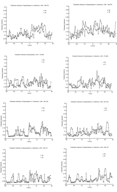
soidal bubbles commonly undergo periodic dilations or random “wobbling” motion [12]. Figure 5 shows the turbulent intensities,

2 2

x x

U u

TI = ′ and ₂

2

x r

U v

TI = ′ , of the

continuous phase at four positions, i.e. x/M = 58.5, 73, 84 and 96, where u′=Ux−Ux and

r

r U

U

v′= − are the fluctuations of the

streamwise and cross-stream velocities of the continuous phase. The turbulent intensity values in the two directions are not the same, meaning that the flow is not isotropic, although in some cases it is close to it. There is a tendency towards a higher degree of isotropicity at the higher void fraction and further downstream from the grid. This could be due to a more uniform cross-stream bubble distribution. The small bubbles in the flow system may have a role similar to that of the grid in creating uniform turbulence in the continuous phase, which is often associated with isotropicity. There is a stronger tendency towards non-isotropicity closer to the grid, which is more clearly seen for the low gas void fraction, which could be because of the unusual flow pattern occurring as the bubbles break through the second grid. The decay of turbulence with increasing distance from the grid (x/M) at the centre of the test section is shown in Figure 6 for both chosen void fractions. The turbulence in the direction of flow is slightly higher than that in the cross-stream direction. Before trying to explain these results it must be mentioned that all these data are based on 1000 images, and that they represent converged mean values according to the frame number graph given in Figure 9. In our previous paper (Moghaddas et al. [10]) it was suggested that a vortex be created behind the tracer injection nozzle, which had a frequency influenced by the interaction of the movements of the bubbles. The results presented above give some additional views on the flow characteristics. The observations

that there are variations in the mean cross-stream velocities, and variations in the turbulence intensities in both the cross-stream and cross-streamwise directions suggest that, in addition to the existence of phenomena that have the character of standing waves, bubbles have pathways that are not random. This is in agreement with the conclusions drawn by Akker that these structures may be the result of wave-like perturbations exhibiting varying degrees of vorticity, while multiphase flows may exhibit a similar vortex shedding frequency as the Karman Vortex Street behind a bluff body. In this system, in addition to the effects of bubble motion and wake behind the injection nozzle, the breakthrough of bubbles in the second circular grid may also cause interfering pressure pulsation.

Concentration

In turbulent flow it is expected that the concentration will fluctuate like velocity, therefore the measured concentration can be decomposed into a mean and a fluctuation value:

= +

C C c (2)

where, for every pixel, C is the

instant-aneous concentration, c is the fluctuation

and C is the average value of the

concentration, which is defined for N

consecutive number of data points by:

1

=

= ∑N i

i

C C

N (3)

(9)

Figure 5. The turbulent intensities in the streamwise direction (TIx) and cross-stream direction (TIr). Each point

represents an average of 1000 images. a) Gas void fraction 1.3% b) gas void fraction 2.4 %.

-30 -20 -10 0 10 20 30 0 0.05 0.1 0.15 0.2 0.25 0.3 0.35 0.4 0.45 0.5

Turbulent intensity of liquid-phase in r-direction, x/M = 73.228

r (mm) Tu rbul en t i nt ens ity

alfa = 2.4% o TIx x TIr

-30 -20 -10 0 10 20 30

0 0.05 0.1 0.15 0.2 0.25 0.3 0.35 0.4 0.45

0.5 Turbulent intensity of liquid-phase in x-direction, x/M = 84.124

r (mm) Tu rb ul ent in tens ity

-30 -20 -10 0 10 20 30

0 0.05 0.1 0.15 0.2 0.25 0.3 0.35 0.4 0.45

0.5 Turbulent intensity of liquid-phase in r-direction, x/M = 84.124

alfa = 2.4% o TIx x TIr -30 -20 -10 0 10 20 30

0 0.05 0.1 0.15 0.2 0.25 0.3 0.35 0.4 0.45

0.5 Turbulent intensity of liquid-phase, x/M = 73.228

r (mm) Tu rbul ent in te ns ity

-30 -20 -10 0 10 20 30

0 0.05 0.1 0.15 0.2 0.25 0.3 0.35 0.4 0.45

-30 -20 -10 0 10 20 30

0 0.05 0.1 0.15 0.2 0.25 0.3 0.35 0.4 0.45

r (mm) Tu rbul ent in te ns ity

-30 -20 -10 0 10 20 30

0 0.05 0.1 0.15 0.2 0.25 0.3 0.35 0.4 0.45

r (mm) Tu rbul ent in tens ity

-30 -20 -10 0 10 20 30

0 0.05 0.1 0.15 0.2 0.25 0.3 0.35 0.4 0.45

r (mm) Tu rb ul en t i nt en si ty

(10)

Iranian Journal of Chemical Engineering, Vol. 3, No. 4 69 55 60 65 70 75 80 85 90 95 100

0 0.05 0.1 0.15 0.2 0.25 0.3

0.35 Turbulent intensity decay for the center of plume, alfa1=1.3 %

x/M

Tu

rbul

en

t i

nt

ens

ity

(a)

55 60 65 70 75 80 85 90 95 100 0

0.05 0.1 0.15 0.2 0.25 0.3

0.35 Turbulent intensity decay for the center of plume, alfa2=2.4%

x/M

Tu

rbul

ent

in

tens

ity

(b)

Figure 6. The turbulence intensity decay downstream

of the grid (o streamwise direction, x cross-stream direction), each point represents an average of 1000 values. a) α =1 3. %, b) α =2 4. %.

the third and fourth moments, are used to

describe the degree of asymmetry (skewness) and heaviness of the tails (flatness) relative to the middle of the distribution.

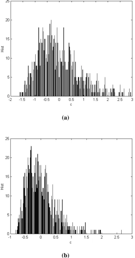
The degree of asymmetry of the distribution of fluctuation values at the centre of the plume is shown in Figure 8a. The skewness is computed using equation (4):

3

1

1 =

⎡ − ⎤

= _⎢ _⎥

δ

⎣ ⎦

∑

N i i k

i

c c S

N (4)

(a)

(b)

Figure 7. Typical PDF histogram of the values of

fluctuation in concentration at a chosen position, x/M = 73 at the centre of the pipe. a) α =1 3. %, b)

2 4 α = . %.

where δ is the deviation of the distribution,

i

c and c_iare the fluctuation in the

concentration and its mean value at each

pixel, and N is the number of images. The

(11)

histograms. The average values calculated for the skewness are approximately 1 and 1.17 for void fractions of 1.3% and 2.4%, respectively. The non-zero values demon-strate an asymmetry of the concentration that is normally associated with intermittency, and are thus in agreement with velocity measurements where flow structures were observed.

The fourth order of moments, flatness, for the fluctuation of concentration, is given in equation (5):

4

1

1 =

⎡ − ⎤

= _⎢ _δ _⎥

⎣ ⎦

∑

N i i l

i

c c F

N (5)

Figure 9 shows the calculated skewness and flatness for the fluctuation in concentration at a chosen point in the centre of the plume. These higher-orders plots show that after 400 images the experimental data are essentially statistically stable. The number of images collected in this study was 1000, which means that these measures should be reasonably reliable for calculating the different moments of the distribution of concentration.

The spread of the tracer is directly affected by the turbulence, and the molecular diffusion is negligible in this kind of flow. The mass transfer calculation can thus be based on the turbulence diffusivity of the flow. In this study we used the Taylor model as an approximation to calculate the spread of the tracer. In this theory the growth of cross-stream distributions of the tracer in the flow direction is related to the distance from the injection point and grid, taking into account the changes in the variance in cross-stream profiles at different positions in the flow direction. The squared values of the variance increase with the distance from the second grid, expressed as x/M. The slope of this growth is a positive value that gives the rate of mass transfer of the plume.

(a)

(b)

Figure 9. Statistical equilibrium for data at a chosen

point, x/M=73, in the centre of the plume. a) Skew-ness, b) flatness.

The self-similarity of the normalised cross-stream profiles of the concentration distribution for both gas flow rates is shown in Figure 10. For ten different streamwise positions downstream of the second grid separated by 7.2 mm in the range of 58.4 < x/M < 94.4, self-similarity was high at the centre of the pipe. The results are normalised to the centre concentration at each streamwise position at the dimensionless radius, r/x. The self-similarity theorem could be useful for spread and mass transfer studies of the tracer.

Figure 11 shows the self-similarity behaviour for cross-stream RMS profiles of con-centration. There is some scattering of the data in the vicinity of the edges of the plume.

Flatness, centre of plume

0 1 2 3 4 5 6

0 200 400 600 800 1000 1200

N

Fl

a

tne

s

alfa 2.4% alfa 1.3%

Skewness, cetre of plume

0 0.2 0.4 0.6 0.8 1 1.2 1.4

0 200 400 600 800 1000 1200

N

Sk

e

w

n

e

ss

alfa 2.4%

alfa 1.3 %

α α

(12)

(a)

(b)

Figure 10. Self-similarity of the cross-stream, mean

concentration profiles. a) α =1 3. %, b) α =2 4. %.

This may be due to different accelerations of the liquid phase at different streamwise positions. The bubbles may have different local properties at different streamwise positions along the test section. The absence of two typical peaks of the void fraction and bubble density profiles between the centre and walls could be another reason for this behaviour.

In Figures 10 and 11 some asymmetry can also be seen in the measured values between the left- and right-hand sides of the pipe, which may be due to the non-uniformity of the light in the bubbly two-phase flow system, or asymmetry of the plume injector. This effect is greater at the edges in the

case

(a)

(b)

Figure 11. Self-similarity of the cross-stream RMS

concentration profiles. a) α =1 3. %, b) α =2 4. %.

of a higher gas void fraction, but there is no effect at the centre of the pipe on the measured parameters.

(13)

Gaussian curves, denoted curve 1 and 2, in order to predict the diffusivity term for different regions of the flow. Curve 1 represents the cross-stream profile at each streamwise location in the central region, which is obtained by subtracting the outer profile from the total curve.

Figure 12. Schematic splitting of the measured data

distribution into two Gaussian curves for the plume in bubbly two-phase flow.

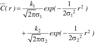
Thus, for each position in the streamwise direction, the mean value of the con-centration can be given by:

1 2

2 1 1

2 2

2 2 2

1 2 2

= −

σ πσ

+ −

σ πσ

k

C( r ) exp( r )

k

exp( r )

(6)

where r is the radius location, C is the

mean value of the concentration, σ₁ and σ₂ are the standard deviations of the two concentration profiles, respectively, and

1

k and k₂ are the experimental constants. In this model, it is assumed that the first Gaussian curve contributes to describing the distribution in the vortex trail created by the injection nozzle. This is similar to the cross-stream profiles of the concentration in the single-phase flow in the grid-generated turbulent flow [13]. As a small liquid flow is

introduced into the pipe at almost the same velocity as the main flow, it could be expected that the vortex trail in the central part would have similar dispersion properties to those in a single-phase flow. The second term on the right side of equation (6) describes the spread of the tracer in the surrounding bubbly continuous phase.

Applying equation (6) to the centre of the plume, it can be written as:

1 2 1 2

1 2

1 0

2 2 2

⎛ ⎞

= = + = _⎜_σ +_σ _⎟

πσ πσ π ⎝ ⎠

c

k k k k

C ( r )

(7)

where Cc is the mean value of the

concentration at the centre of the plume. Using the dimensionless radius, r/x, and dividing equation (6) by equation (7), the self-similarity equation can be obtained:

2 2

1 2 ₂

2 1 1 2 1

2 2

2 1 ₂

2

1 1

2 1

2

η ₌⎛ ⎞ ⎡ _σ ₋ _η

⎜ _{σ + σ} ⎟ ⎢ _σ

⎝ ⎠ ⎣

⎤

+ σ − _σ η _⎥ η =

⎦ c

C ( )

k exp( x ) ,

k k

C

r

k exp( x )

x

(8)

where x and η give the location in

streamwise and dimensionless cross-stream co-ordinates, respectively.

It is well known that the displacement of the spread is analogous to the standard deviation

(σ ), which is the width of the normal

distribution curve at its inflection point. In the present study Taylor’s theory was used as an approximation to calculate the turbulent diffusion coefficient. According to this theory, the variation of variance of the mean concentration profile, _σ2_{, can be given as}

follows [14]:

2

0

2

σ = DT

x

U (9)

(14)

flow and DT is the turbulent diffusion

coefficient. So, the turbulent diffusion coefficient can be written as follows:

2 0

4

σ =

T

d( ) U

D

dx (10)

or

2 0

4

σ =

T

U d( ) D

M d( x / M ) (11)

As mentioned above, the total spread can be described by two superimposed Gaussian distributions, where σ₁ describes the spread

in the central region, and σ₂ is used to

describe the spread in the outer regions. The calculation procedure for the spreading rate based on observations is to apply equation (6) at each streamwise position, separately. Therefore, commercial curve-fitting software was used to determine the four coefficients,

1 2 1 ,k ,σ

k , and σ₂ of the equation for each

cross-stream profile at a streamwise range of 58.4 < x/M < 94.4.

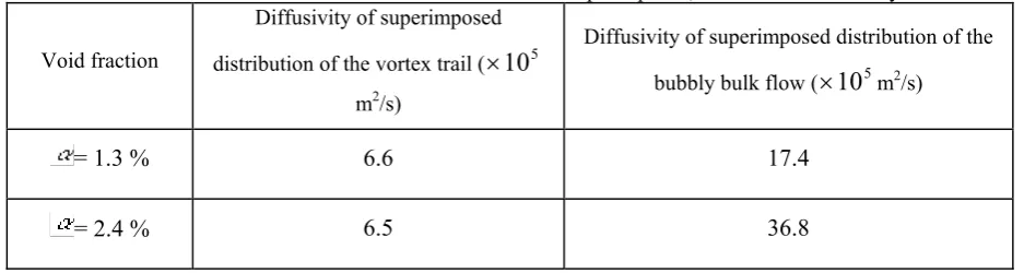
Figure 13 shows the variation of the calculated values of the variances of the Gaussian profiles in the downstream direction. It can be concluded that the width of the profiles, measured at their inflection points, for both the central and outer regions increases linearly with x/M. Figure 13a shows the spread of the profiles in the central region for the two void fractions studied. In this region there is no difference between the slopes of the lines, which show that the effect of increasing the void fraction on the rate of spread is negligible. The slopes of the corresponding lines for the bulk region show large differences between the two cases, as can be seen in Figure 13b. Finally, the turbulent spreading coefficients are cal-culated using the calcal-culated slopes from Figure 13 and equation (11). Table 1 shows the values of the turbulent diffusion coefficient for both regions. Almost doubling the gas void fraction has no effect on the

spread of the tracer in the central region, while there was a strong effect on the spread in the bulk of the bubbly flow.

(a)

(b)

Figure 13. The variation of the variance of the

cross-stream concentration profiles. a) Outer part of the plume, b) central part of the plume.

The diffusivity of the superimposed distribution in the vortex trail, forming part of the observed plume, show very close values to those obtained for the single-phase flow (6.2×10-5 m2/s) [10]. As a final result one can say that the spread of the tracer in the vortex trail is almost independent of the flow in the bubbly bulk region for the system studied. As the tracer distributed from the tip of the injection nozzle has the same speed as the continuous liquid phase of the main continuous flow into the channel, the distribution of the tracer, the bubble void fraction, and the vortex shedding behind the nozzle may explain this result.

slope = 0.4 Dti=65.5 mm^2/s slope = 0.399

Dti=65 mm^2/s

0 5 10 15 20 25

55 65 75 85 95 105

x/M

Si

g

m

a

1

^2

alfa = 1.3 %

alfa = 2.4 %

slope = 1.068 Dto = 173.8 mm^2/s slope = 2.261

Dto = 367.5 mm^2/s

0 20 40 60 80 100 120 140

55 65 75 85 95 105

x/M

Si

g

m

a

2

^2

alfa = 1.3 %

alfa = 2.4 % α α

(15)

Table 1. The calculated turbulent diffusion coefficient for both superimposed, vortex trail and bubbly bulk flow.

Void fraction

Diffusivity of superimposed distribution of the vortex trail (×105

m2_/s)

Diffusivity of superimposed distribution of the bubbly bulk flow (×105m2_/s)

= 1.3 % 6.6 17.4

= 2.4 % 6.5 36.8

Conclusion

The spread of a tracer in bubbly two-phase flow has been studied, and a new mathe-matical model suggested to analyse the cross-stream distribution and the self-similarity of the mean values of tracer concentration in two-phase flow. This allows one to distinguish between diffusion phenomena in the grid-generated turbulence, including bubbles, and the special diffusion phenomena occurring due to vortex shedding. The diffusivity is strongly influenced by the presence of the gas bubbles in the system investigated; with only 1.3% gas a threefold increase was observed compared to single-phase flow. To investtigate the effect of gas void fraction on the mixing characteristics, two different gas flow rates were studied. Nearly isotropicity for the continuous-phase of the grid-generated turbulence in the bubbly two-phase flow is observed by calculating the turbulent intensity for both cross-stream and streamwise co-ordinates. Upon increasing the void fraction the turbulence in the liquid phase tends to be more isotropic. This could be due to the uniform distribution of the bubbles in the higher gas flow, or to the fact that more bubbles create more small eddies that are associated with isotropicity. Near self-similar behaviour of the cross-stream mean and RMS values of the concentration was observed.

Acknowledgements

The authors are grateful for the partial

financial support from the Iranian Ministry of Science, Research and Technology and the Swedish Foundation for Strategic Research, Program for Multiphase Flow.

References

1. Serizawa, A., Kataoka, I. and Michiyoshi, I. (1974) Turbulence structure of air-water bubbly flow-I. Measuring techniques. International J. Multiphase Flow 2:221-233. 2. Beyerlein, S. W., Cossmann, R. K. and

Richter, H. J. (1985) Prediction of bubble concentration profiles in vertical turbulent two-phase flow. International J. Multiphase Flow 11:629-641.

3. Hibiki, T., Hogsett, S. and Ishii, M. (1998) Local measurement of interfacial area, interfacial velocity and liquid turbulence in two-phase flow. Nuclear Engineering and Design 184: 287-304.

4. Dizallas, H., Michele, V. and Hempel, D. C. (2000) Measurement of local phase holdups in a two- and three-phase bubble column. Chem. Eng. Technol. 23: 877-884.

5. Bouaifi, M., Hebrard, G., Bastoul, D. and Roustan, M. (2001) A comparative study of gas hold-up, bubble size, interfacial area and mass transfer coefficients in stirred gas-liquid reactors and bubble columns. Chemical engineering and processing 40: 97-111.

6. Lance, M., Marie, J. L. and Bataille, J. (1990) Homogeneous Turbulence in bubbly Flows. Journal of Fluids Engineering 113: 295-300. 7. Panidis, T. and Papailiou, D. D. (2000) The

(16)

Iranian Journal of Chemical Engineering, Vol. 3, No. 4 75 8. Moghaddas, J. S., Trägårdh, C., Kovacs, T.

and Östergren, K. (2002a) A new method for measuring concentration of a fluorescent tracer in bubbly gas-liquid flows. Experi-ments in Fluids 32: 728-729.

9. Moghaddas, J. S., Trägårdh, C. and Östergren, K. (2002b) Use of a simultaneous PLIF-PLIF technique to overcome optical problems in concentration measurements in two-phase bubbly system. Advances in Fluid Mechanics IV, WITPRESS: 427-437.

10. Moghaddas, J. S. and et al. (2004), Comparison of the mixing process in single- and two-phase grid-generated turbulent flow systems, Chemical Engineering and Tech-nology, Vol. 27-No 6, 662-670.

11. Brenn, G., Braeske, H., Zivkovic, G. and Durst, F. (2003) Experimental and numerical invest-tigation of liquid channel flows with dis-persed gas and solid particles. Interna-tional Journal of Multiphase Flow 29: 219-247.

12. Clift, R., Grace, J. R, and Weber, M. E. (1978) Bubbles, Drops, and particles. Academics Press, Inc. New York.

13. Lemoine, F., Antoine, Y., Wolff, M. and Lebouche′, M. (2000) Some experimental investigations on the concentration variance and its dissipation rate in a grid generated turbulent flow. International journal of Heat Mass Transfer 43: 1187-1199.