Vol. 4, No. 2, Year 2012 Article ID IJIM-00207, 11 pages Research Article
Estimated Returns to Scale with Interval Data in
Parallel Manufacturing Systems with Shared
Resources
S. Kordrostamia∗, A. Amirteimoorib, O. Azmayandeha, Z. Bakhodaa
(a)Department of Applied Mathematics,Lahijan Branch,Islamic Azad University, Lahijan , Iran (b)Department of Applied Mathematics, Rasht Branch,Islamic Azad University, Rasht, Iran
———————————————————————————————— Abstract
Many models in DEA have been proposed to estimate returns to scale. Determining the nature of returns to scale has considerable of importance in the theory of production. Knowing the fact that returns to scale is a constant, ascending or descending decision making unit, proper actions can be performed to develop the decision making units. In this study, the efficiency of parallel production systems with shared resources is evaluated such that the data is inexact and interval, so the function of these systems is interval too. Then a model is proposed to estimate returns to scale of interval data on these systems; when the data is inexact, the nature of returns to scale of these units is inexact too, so returns to scale is estimated as multiple in best and worst conditions.
Keywords: Returns to scale; Parallel systems; Interval data; Efficiency.
————————————————————————————————–
1
Introduction
Determining the nature of returns to scale of decision making units in the production theory is of high importance; Knowing the fact that returns to scale is a constant, ascending or descending decision making unit, proper actions can be carried out. One of the research topics with functional value is to estimate the nature of returns to scale of decision making units when the input and output data is inexact and interval. Kao (2006) believed that when the input and output data is inexact and interval, the efficiency should be interval too, so we should define an interval efficiency for decision-making units with inexact data. In the real world there are systems which are composed of independent production units. These systems use input data to produce output. Kao (2008) evaluated the performance of the production systems which are composed of parallel production units. Kordrostami et al (2010) considered production systems which are composed of parallel subunits such that each subunit uses given inputs and part of shared resources to produce the final output.
∗Corresponding author. Email address: [email protected]
But when the input and output data is inexact, we can propose models to evaluate the performance of these systems in the most optimistic and pessimistic cases. In this paper, we evaluate the efficiency of parallel production systems with shared resources when the data is inexact and interval. Also, we estimate returns to scale of these systems. Moreover, we believe that when the input and output data is inexact, returns to scale are inexact too, so returns to scale is estimated as multiple in best and worst conditions. The structure of this paper is as follows: In the next section, we provide the related models. In the third section, the models to evaluate the efficiency of the parallel production systems with shared resources and the estimation of returns to scale in these systems are provided. In order to analyze the proposed models, we provide a practical example in the fourth Section, and finally in the last section the conclusion is drawn.
2
The related models
In this section we briefly explain the models used in this paper.
2.1 Parallel model with shared resources
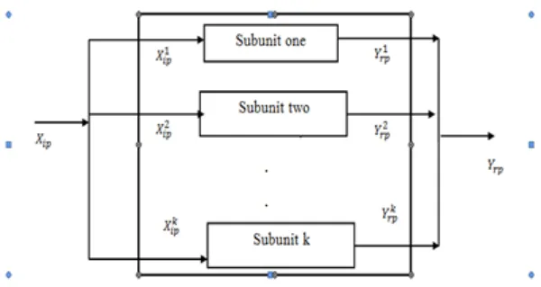
Consider a parallel production system as shown in Figure 1. Assume that we have n decision making units, and each unit has T parallel subunits where each subunit uses its own input and the shared resources. In particular, t−th subunit ofDM U P uses its own inputXp(t)and part of the shared resource ofXp(s). Assume thatXp(s,t)is part of the shared input of Xp(t) which is assigned to thet−th subunit.
The process is shown in Figure 1. Yp(t) is the produced output of the t−th subunit. Clearly, we have:Xp(s)=∑Tt=1Xp(s,t).
Figure 1. The parallel production system, where a DMUp has k production units.
The production possibility set (P P S) of thet−thsubunit under the assumption of vari-able returns to scale is as follows:
Tv(t)={(X(t), Y(t), X(s,t)) : n
∑
j=1
λjXj(t)≤X(t), n
∑
j=1
λjYj(t)≥Y(t), n
∑
j=1
λjXj(s,t) ≤X(s,t)},
n
∑
j=1
To calculate the technical efficiency of DMUP, we are to solve the following programming problem:
min∑Tt=1wtθt+ ´2θt
s.t.
∑n
j=1λjXj(t)≤θtXp(t), t= 1, ..., T
∑n
j=1λjXj(s,t)≤θ´tXp(s,t), t= 1, ..., T
∑n
j=1λjYj(t)≥Y
(t)
p , t= 1, ..., T,
∑n
j=1λj = 1, λj ≥0, j= 1, ..., n,
θt≤1, θ´t≤1.
(2.1)
The objective function of the above model is a weighted set of Ep(t)= θt+ ´2θt,(t= 1, ..., T).
wts are the assumed coefficients by a specific user and we have:
∑T
t=1wt = 1. In this
model,Ep(t)is the bonus of the efficiency of t-th subunit which is equal to the average ofθtand ´θtorE(pt)= θt+ ´2θt.AlsoEpis the bonus of the efficiency of the whole system i.e.Ep=
∑T t=1wt
θt+ ´θt
2 =
∑T t=1wtE
(t)
p . Moreover, we can show the feasibly and boundedness of the linear programming problem (2.1).
2.2 The estimation of the returns to scale in DEA
In this section, we examine a model proposed by Khodabakhshi, et al (2010). They devel-oped a model to estimate returns to scale in data envelopment analysis as follows. They tried to use the proposed model to make a non-efficient(ξxo, ξyo)to determine returns to scale (xo, yo).There, if the non-efficiency (ξxo, ξyo) increases, ξin one level, returns to scale will increase, and if it decreases, ξin one level, returns to scale will decrease as well. If(ξxo, ξyo) is never non-efficient, returns to scale are constant. The presented model is as follows:
max 1s−+ 1s+
s.t.
∑n
j=1λjxj+s− =ξxo,
∑n
j=1λjyj−s+=ξyo,
∑n
j=1λj = 1
λj ≥0, j= 1, ..., n, s−, s+≥0
The following theorem provides returns to scale with model (2.2).
Theorem 2.1. The assumption DM Uo with the input output mix (xo, yo) are efficient.
The following conditions provide returns to scale of DM Uo with model (2.2).
A-The optimal amount of objective function is greater than zero and ξ∗ >1 if and only if DM Uo has increasing returns to scale.
B - The optimal amount of objective function is greater than zero and ξ∗ <1 if and only if DM Uo has decreasing returns to scale.
C - The optimal amount of objective function is zero and this is possible if and only if DM Uo has a constant returns to scale.
3
Proposed Models
3.1 The Parallel Model with Shared Resources on Interval Data
Consider a parallel production system as shown in Figure 1. Suppose we havenDM U s, and each DM U has T parallel subunits, so that each subunit has its own inputs and all subunits use a shared resource. In particular, the t−th subunit of DM UP uses its own inputs Xp(t) and a part of the shared inputs Xp(s) . Suppose Xp(s,t) is a part of the shared inputs Xp(s) dedicated to subunit t. The output produced by subunit t is Yp(t) clearly, we have Xp(s) =
∑T t=1X
(s,t)
p .Also assume that the input and outputs are known to lie within bounded intervals, i.e. Xp(t) ∈ [LXp(t),UXp(t)] , Xp(s,t) ∈ [LXp(s,t),UXp(s,t)] andYp(t) ∈[LYp(t),UYp(t)] .
Also, the provided parallel model with shared sources in section 2-2, i.e. model (1) is considered as the basis of the work.
Definition 3.1. Suppose [LXj(t),UXj(t)], [LXj(s,t),UXj(s,t)] and [LYj(t),UYj(t)] are the own input, shared input and output of DM Uj, respectively. The best situation of DM Up is
defined as follows:
Xp(t)=LXp(t), Xp(s,t)=LXp(s,t), Yp(t)=U Yp(t)
Xj(t) =U Xj(t), Xj(s,t)=U Xj(s,t), Yj(t)=LYj(t), j̸=p, j= 1, ..., n
Definition 3.2. Suppose [LXj(t),UXj(t)], [LXj(s,t),UXj(s,t)] and [LYj(t),UYj(t)] are the own input, shared input and output of DM Uj , respectively. The best situation of DM Up is
defined as follows:
Xp(t)=U Xp(t), Xp(s,t)=U Xp(s,t), Yp(t)=LYp(t)
Xj(t)=LXj(t), Xj(s,t)=LXj(s,t), Yj(t)=U Yj(t), j ̸=p, j= 1, ..., n
cal-culated by using the following model:
θL= min∑Tt=1wtθt+ ´2θt
s.t.
∑n
j=1,j̸=pλLjX
(t)
j +λUpX
(t)
p +s−(t)=θtUXpt, t= 1, ..., T
∑n
j=1,j̸=pλLjX
(s,t)
j +λUpX
(s,t)
p +s−´(t)= ´θt U
Xp(s,t), t= 1, . . . , T
∑n
j=1,j̸=pλUj Y
(t)
j +λLpY
(t)
p −s+(t)=LYp(t), t= 1, . . . , T
∑n
j=1λj = 1,
θt≤1, t= 1, ..., T
´
θt≤1, t= 1, ..., T
λj ≥0, s−(t),s−´(t), s+(t)≥0 j= 1, ..., n
(3.3)
Also, the upper bound of the efficiency score can be calculated by using the following model:
θU = min∑Tt=1wtθt+ ´2θt
s.t.
∑n
j=1,j̸=pλUj X
(t)
j +λLpX
(t)
p +s−(t)=θtLXpt, t= 1, ..., T
∑n
j=1,j̸=pλUj X
(s,t)
j +λLpX
(s,t)
p +s−´(t)= ´θt L
Xp(s,t), t= 1, . . . , T
∑n
j=1,j̸=pλLjY
(t)
j +λUpY
(t)
p −s+(t)=U Yp(t), t= 1, . . . , T
∑n
j=1λj = 1,
θt≤1, t= 1, ..., T
´
θt≤1, t= 1, ..., T
λj ≥0, s−(t),s−´(t), s+(t)≥0 j= 1, ..., n
(3.4)
θL together with θU constitute the efficiency interval as [θL, θU] that covers all possible efficiency scores for the whole system. Also, in model(3.3) UEpt = Uθt+Uθ´t
2 is the upper efficiency score of the subunit t, and in model (3.4)LEpt = Lθt+Lθ´t
3.2 The Estimation of Returns to Scale with Interval Data
In parallel production systems with shared resources as shown in the previous section, when the data in the parallel production systems with shared resources is interval, the efficiency is interval too. So when the data is interval, a return to scale is estimated as multiple in best and worst conditions. The models to estimate returns to scale in best and worst conditions are defined as follows:
max 1s−(t)+ 1 ´s−(t)+ 1s+(t)
s.t.
∑n
j=1,j̸=pλLjX
(t)
j +λUpX
(t)
p +s−(t) =ξUXpt, t= 1, ..., T
∑n
j=1,j̸=pλLjX
(s,t)
j +λUpX
(s,t)
p +s−´(t)=ξUXp(s,t), t= 1, . . . , T
∑n
j=1,j̸=pλUjY
(t)
j +λLpY
(t)
p −s+(t)=ξLYp(t), t= 1, . . . , T
∑n
j=1λj = 1,
λj ≥0, s−(t),s−´(t), s+(t)≥0 j= 1, ..., n
(3.5)
max 1s−(t)+ 1 ´s−(t)+ 1s+(t)
s.t.
∑n
j=1,j̸=pλUj X
(t)
j +λLpX
(t)
p +s−(t)=ξLXpt, t= 1, ..., T
∑n
j=1,j̸=pλUj X
(s,t)
j +λLpX
(s,t)
p +s−´(t)=ξLXp(s,t), t= 1, . . . , T
∑n
j=1,j̸=pλLjY
(t)
j +λUpY
(t)
p −s+(t)=ξUYp(t), t= 1, . . . , T
∑n
j=1λj = 1, λj ≥0, s−(t),s−´(t), s+(t) ≥0 j= 1, ..., n.
(3.6)
Definition 3.4. Suppose DM UP with input-output (Xp, Xp(s), Yp) is efficient. Therefore,
we have:
(i) The optimal value of the objective functions of models (3.5) and (3.6) are greater than zero and ξ∗ >1 if and only if DM UP has increasing returns to scale (IRS).
(ii) The optimal value of the objective functions of models (3.5) and (3.6) are greater than zero and ξ∗ <1 if and only if DM UP has decreasing returns to scale (DRS).
(iii) The optimal value of the objective functions of models (3.5) and (3.6) are zero if and only if DM UP has constant returns to scale (CRS).
4
The Applied Study on Iran’s Bank
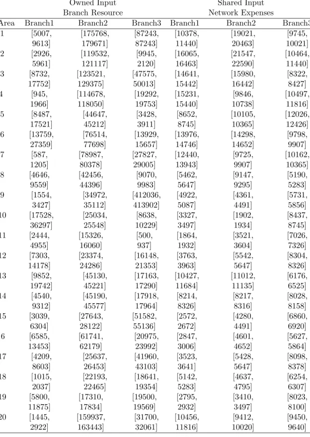
Here each area is composed of three branches and each branch uses the network expenses as shared input and branch resources as the owned input to produce payment facilities (loans) as output. In Table (1),(2) we see the input and output data.
Table 1. The input-output data of 20 areas of Iran’s Bank.
Owned Input Shared Input
Branch Resource Network Expenses
Area Branch1 Branch2 Branch3 Branch1 Branch2 Branch3
1 [5007, [175768, [87243, [10378, [19021, [9745,
9613] 179671] 87243] 11440] 20463] 10021]
2 [2926, [119532, [9945, [16065, [21547, [10464,
5961] 121117] 2120] 16463] 22590] 11440]
3 [8732, [123521, [47575, [14641, [15980, [8322,
17752] 129375] 50013] 15442] 16442] 8427]
4 [945, [114678, [19292, [15231, [9846, [10497,
1966] 118050] 19753] 15440] 10738] 11816]
5 [8487, [44647, [3428, [8652, [10105, [12026,
17521] 45212] 3911] 8745] 10365] 12426]
6 [13759, [76514, [13929, [13976, [14298, [9798,
27359] 77698] 15657] 14746] 14652] 9907]
7 [587, [78987, [27827, [12440, [9725, [10162,
1205] 80378] 29005] 13943] 9907] 10365]
8 [4646, [42456, [9070, [5462, [9147, [5190,
9559] 44396] 9983] 5647] 9295] 5283]
9 [1554, [34972, [412036, [4922, [4361, [5731,
3427] 35112] 413902] 5087] 4491] 5856]
10 [17528, [25034, [8638, [3327, [1902, [8437,
36297] 25548] 10229] 3497] 1934] 8745]
11 [2444, [15326, [500, [1864, [3521, [7026,
4955] 16060] 937] 1932] 3604] 7326]
12 [7303, [23374, [16148, [3763, [5542, [8304,
14178] 24286] 21353] 3963] 5647] 8326]
13 [9852, [45130, [17163, [10427, [11012, [6176,
19742] 45221] 17290] 11684] 11135] 6525]
14 [4540, [45190, [17918, [8214, [8217, [8028,
9312] 45577] 17964] 8326] 8316] 8158]
15 [3039, [27643, [51582, [2572, [4280, [6860,
6304] 28122] 55136] 2672] 4491] 6920]
16 [6585, [61741, [20975, [2847, [4601, [5627,
13453] 62179] 23992] 3006] 4652] 5864]
17 [4209, [25637, [41960, [3523, [5428, [8098,
8603] 26453] 43103] 3641] 5647] 8378]
18 [1015, [22193, [18641, [5142, [4637, [6254,
2037] 22465] 19354] 5283] 4795] 6307]
19 [5800, [17310, [19500, [2795, [3410, [8023,
11875] 17834] 19569] 2932] 3497] 8100]
20 [1445, [159937, [31700, [10456, [9412, [9450,
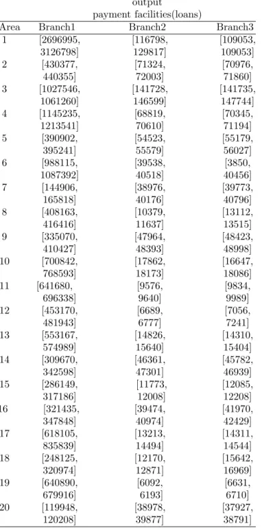
Table 2. The interval output data for the 20 area of Iran’s Bank. output
payment facilities(loans)
Area Branch1 Branch2 Branch3
1 [2696995, [116798, [109053,
3126798] 129817] 109053]
2 [430377, [71324, [70976,
440355] 72003] 71860]
3 [1027546, [141728, [141735,
1061260] 146599] 147744]
4 [1145235, [68819, [70345,
1213541] 70610] 71194]
5 [390902, [54523, [55179,
395241] 55579] 56027]
6 [988115, [39538, [3850,
1087392] 40518] 40456]
7 [144906, [38976, [39773,
165818] 40176] 40796]
8 [408163, [10379, [13112,
416416] 11637] 13515]
9 [335070, [47964, [48423,
410427] 48393] 48998]
10 [700842, [17862, [16647,
768593] 18173] 18086]
11 [641680, [9576, [9834,
696338] 9640] 9989]
12 [453170, [6689, [7056,
481943] 6777] 7241]
13 [553167, [14826, [14310,
574989] 15640] 15404]
14 [309670, [46361, [45782,
342598] 47301] 46939]
15 [286149, [11773, [12085,
317186] 12008] 12208]
16 [321435, [39474, [41970,
347848] 40974] 42429]
17 [618105, [13213, [14311,
835839] 14494] 14544]
18 [248125, [12170, [15642,
320974] 12871] 16969]
19 [640890, [6092, [6631,
679916] 6193] 6710]
20 [119948, [38978, [37927,
120208] 39877] 38791]
We applied the parallel models (3.3) and (3.4) for these data, and we calculated the lower and upper bounds of efficiency for these 20 areas and their subordinated branches. With the use of models (3.5) and (3.6) and definition 4 we estimate returns to scale of the areas in both best and worst conditions. We assume weights as: w1 = 0.5, w2 = 0.3, w3 = 0.2.
Table 3. The results of the returns to scale estimation and the efficiency interval for 20 ar-eas of Iran’s Bank.
Area E1 E2 E3 Efficiency in Efficiency in RTS in the RTS in the
the worst the best worst best situation situation situation situation
1 [1.0000, [1.0000, [1.0000, 1.0000 1.0000 CRS CRS
1.0000] 1.0000] 1.0000]
2 [1.0000, [1.0000, [1.0000, 1.0000 1.0000 CRS CRS
1.0000] 1.0000] 1.0000]
3 [1.0000, [1.0000, [1.0000, 1.0000 1.0000 CRS CRS
1.0000] 1.0000] 1.0000]
4 [1.0000, [1.0000, [1.0000, 1.0000 1.0000 CRS CRS
1.0000] 1.0000] 1.0000]
5 [1.0000, [1.0000, [1.0000, 1.0000 1.0000 CRS CRS
1.0000] 1.0000] 1.0000]
6 [0.2129, [0.5216, [0.8669, 0.4363 1.0000 DRS CRS
1.0000] 1.0000] 1.0000]
7 [0.7560, [0.7510, [0.7206, 0.7474 1.0000 IRS CRS
1.0000] 1.0000] 1.0000]
8 [1.0000, [1.0000, [1.0000, 1.0000 1.0000 IRS IRS
1.0000] 1.0000] 1.0000]
9 [1.0000, [1.0000, [1.0000, 1.0000 1.0000 CRS CRS
1.0000] 1.0000] 1.0000]
10 [1.0000, [1.0000, [1.0000, 1.0000 1.0000 CRS CRS
1.0000] 1.0000] 1.0000]
11 [1.0000, [1.0000, [1.0000, 1.0000 1.0000 CRS CRS
1.0000] 1.0000] 1.0000]
12 [0.3214, [0.6273, [0.4336, 0.4356 0.5926 DRS DRS
0.5959] 0.6687] 0.4701]
13 [0.1969, [0.5002, [0.6448, 0.3775 0.7210 IRS IRS
0.6339] 0.8054] 0.8119]
14 [0.5394, [0.8989, [0.8171, 0.7028 1.0000 IRS CRS
1.0000] 1.0000] 1.0000]
15 [0.5815, [0.7361, [0.5186, 0.6153 1.0000 IRS IRS
1.0000] 1.0000] 1.0000]
16 [1.0000, [1.0000, [1.0000, 1.0000 1.0000 CRS CRS
1.0000] 1.0000] 1.0000]
17 [0.4645, [0.7002, [0.4447, 0.5315 1.0000 DRS CRS
1.0000] 1.0000] 1.0000]
18 [1.0000, [1.0000, [1.0000, 1.0000 1.0000 IRS CRS
1.0000] 1.0000] 1.0000]
19 [0.4338, [0.9337, [0.4508, 0.5872 1.0000 DRS CRS
1.0000] 1.0000] 1.0000]
20 [0.5788, [0.6064, [0.7192, 0.5967 1.0000 IRS IRS
1.0000] 1.0000] 1.0000]
the last two columns of Table 2, returns to scale of areas are given in the best and worst conditions. According to the table of results, it can be seen that areas 1, 2, 3, 4, 5, 8, 9, 10, 11, 16 and 18 are efficient; namely, the efficiencies of these areas are equal to 1 in each two situations. But it can be seen that areas 6, 7, 14, 15, 19 and 20 are efficient in the upper bound and inefficient in the lower bound. Also, it can be observed that the returns to scale are not precise, and they are estimated as multiple. In areas 6, 7, 14, 17, 18 and 19 it is shown that the returns to scale are not estimated precisely. For example, area 6 has decreasing returns to scale in the worst situation and it has constant returns to scale in the best situation.
5
Conclusion
In this paper, models for calculating efficiency and estimating returns to scale in parallel production systems with shared resources were presented on imprecise data where the inputs and outputs were interval. With the use of these models, the efficiency of subunits and the whole system was obtained as interval and inexact. Then, the data was applied on 20 areas of Iran’s Banks. In this paper, returns to scale were not exact and were estimated as multiple.
References
[1] A. Charnes, A. Cooper, WW. Rhodes, E. Measuring Efficiency of Decision Making Units, European Journal of Operational Research 1 (1978) 429-444.
[2] WD. Cook, M. Kress, LM. Seiford, On the use of ordinal data in data envelopment analysis, Journal of the Operational Research Society 44 (1993) 133-140.
[3] WW. Cooper, KS. Park, G. Yu, IDEA and AR-IDEA: Models for dealing with im-precise data in DEA, Management Science 45 (1999) 597-607.
[4] D. Primont, Efficiency Measures for Multiplan Firms, Operations Research Letters 3 (1984) 257-260.
[5] C. Kao, PL. Chang, SN. Hwang, Data Envelopment Analysis in Measuring the Ef-ficiency of Forest Management, Journal of Environmental Management 38( 1993) 73-83.
[6] C. Kao, the Efficiency Measurement for Parallel Production Systems, European Jour-nal of OperatioJour-nal Research 4 (2008) 56-66.
[7] C. Kao, Interval efficiency measures in data envelopment analysis with imprecise data, European Journal of Operational Research 174 (2006) 1087-1099 .
[8] C. Kao, Measuring the Efficiency of Forest District with Multiple Working Circles, Journal of Operational Research Society 49 (1998) 583-590.