ESTIMATING AND INTERPRETING PROBABILITY DENSITY FUNCTIONS

(1)

November 1999

ESTIMATING AND INTERPRETING

PROBABILITY DENSITY FUNCTIONS

Proceedings of the workshop

held at the BIS on 14 June 1999

BANK FOR INTERNATIONAL SETTLEMENTS

Monetary and Economic Department

(2)

papers and considered preliminary drafts of any subsequent publication. They are reproduced here to make them easily available to anyone having an interest in the subject of the workshop. Although all papers have been screened for relevance to the subject matter of the workshop, they have not been subject to a rigorous refereeing process nor edited for form or content by the Bank for International Settlements.

Copies of publications are available from:

Bank for International Settlements Information, Press & Library Services CH-4002 Basel, Switzerland

Fax: +41 61 / 280 91 00 and +41 61 / 280 81 00

This publication is available on the BIS website (www.bis.org).

© Bank for International Settlements 1999.

(3)

November 1999

ESTIMATING AND INTERPRETING

PROBABILITY DENSITY FUNCTIONS

Proceedings of the workshop

held at the BIS on 14 June 1999

BANK FOR INTERNATIONAL SETTLEMENTS

Monetary and Economic Department

(4)

(5)

Participants in the meeting

Foreword

P H K Chang (Credit Suisse First Boston) and W R Melick (Kenyon College): Background note

First session – Estimation techniques

W R Melick (Kenyon College): Results of the estimation of implied PDFs from a common dataset

N Cooper (Bank of England): “Testing techniques for estimating implied RNDs from the prices of European-style options”

Discussants: H Neuhaus (European Central Bank) and J M Berk (Netherlands Bank)

S Coutant (Bank of France): “Implied risk aversion in option prices using Hermite polynomials”

Discussant: R Bliss (Federal Reserve Bank of Chicago)

D J McManus (Bank of Canada): “The information content of interest rate futures options”

Discussants: J Mahoney (Federal Reserve Bank of New York) and R Violi (Bank of Italy)

Second session – Applications and economic interpretation

G Gemmill and A Saflekos (City University Business School): “How useful are implied distributions? Evidence from stock-index options”

Discussants: S Shiratsuka (Bank of Japan) and R Wouters (Belgian National Bank)

J M Campa (New York University), P H K Chang (Credit Suisse First Boston) and J F Refalo (New

York University): “An options-based analysis of emerging market exchange rate expectations:

Brazil’s Real Plan, 1994–1997”

Discussants: P Söderlind (Stockholm School of Economics) and C Manzano (Bank of Spain)

B Adão and J Barros Luís (Bank of Portugal): “Interest rate spreads implicit in options: Spain and Italy against Germany”

(6)

(7)

Name Affiliation E-mail

Ms J Aguilar Bank of Sweden Mr J Berk Netherlands Bank

Mr R Bliss Federal Reserve Bank of Chicago Mr V Brousseau European Central Bank

Mr J Campa New York University Mr N Cooper Bank of England Ms S Coutant Bank of France Mr T Flury Swiss National Bank

Mr G Gemmill City University Business School Mr M Loretan Board of Governors of the Federal

Reserve System Mr J Barros Luís Bank of Portugal

Mr J Mahoney Federal Reserve Bank of New York Mr A Malz RiskMetrics

Ms M C Manzano Bank of Spain Mr D McManus Bank of Canada Mr W Melick Kenyon College Mr H Neuhaus European Central Bank Mr S Shiratsuka Bank of Japan

Mr P Söderlind Stockholm School of Economics Mr C Upper Deutsche Bundesbank

Mr R Violi Bank of Italy

Mr R Wouters Belgian National Bank

BIS: Mr R Filosa Mr G Galati Mr E Remolona

[email protected] [email protected] [email protected] [email protected] [email protected]

[email protected] [email protected] [email protected] [email protected]

[email protected] [email protected]

[email protected] [email protected] [email protected]

(8)

(9)

In recent years, central banks have increasingly used option markets to construct measures of market conditions and market participants’ expectations. Most recently, techniques have been developed that use option prices to estimate or recover the entire expected distribution (probability density function, PDF) of future financial asset prices such as interest rates, exchange rates and equity prices. These PDFs allow for a more complete characterisation of the state of market expectations.

There are a number of different techniques currently used to estimate PDFs from option prices, and in some cases they have produced different results. There is at this point no consensus on which technique should be used in which situation. Moreover, opinion differs as to how PDFs should be interpreted. As the use of estimated PDFs has become increasingly popular in the central banking community, the BIS decided to organise a one-day workshop on estimation and interpretation of PDFs. The workshop was held in Basel on 14 June 1999 and organised by Gabriele Galati of the BIS and William Melick of Kenyon College, Ohio; it brought together experts from central banks, academia and the investment community. The background paper by Kevin Chang and William Melick provides an overview of the issues involved in the estimation and interpretation of PDFs.

The workshop was divided into two sessions. The first session addressed issues related to the estimation techniques. Before the workshop, participants received a common data set of settlement price data for options on eurodollar futures between 1 September 1998 and 30 November 1998. Participants were asked to estimate an implied PDF using their own technique for each trading day in the data set and to provide a standard set of summary statistics. The results, which are summarised in a note by William Melick, were discussed at the beginning of the first session.

Three papers were then presented. The paper by Neil Cooper (Bank of England) compared the accuracy of alternative estimation techniques using simulated distributions and applying a Monte Carlo test. The paper by Sophie Coutant (Bank of France) provided a theoretical framework for separating the risk-neutral density function from a risk-aversion function. She then estimated these functions using data on CAC options. Des McManus (Bank of Canada) applied alternative techniques to estimate PDFs from eurodollar futures and used different statistics to evaluate their performance. The second session focused on applications of PDFs and on issues related to their economic interpretation. Gordon Gemmill (City University Business School) analysed the behaviour of PDFs estimated from FT-SE 100 option prices around a number of “crash episodes” and several election dates in the United Kingdom and evaluated their predictive content. José Campa (New York University), Kevin Chang (Credit Suisse First Boston) and James Refalo (New York University) used option data from Brazil to describe expectations of the real/dollar exchange rate and analysed the credibility of different exchange rate regimes. Finally, the paper by Jorge Barros Luís and Bernardino Adão (Bank of Portugal) used PDFs to evaluate expectations regarding interest rate convergence in Europe in the run-up to monetary union.

(10)

(11)

1

Background note

P H Kevin Chang and William R Melick

Starting in the late 1980s, financial and economic researchers became increasingly sophisticated in their attempts to analyze market expectations embedded in option prices. Moving beyond the study of implied Black-Scholes volatilities, this body of work has focused on the recovery of either the stochastic process followed by the underlying asset price or the density function from which the asset price at expiration will be drawn. The workshop was meant to share information and results on the latter exercise, the estimation of terminal (at expiration) probability density functions (PDFs) implied by option prices. Toward that end, this note is meant to provide some context reading the papers presented at the workshop. The first section of the note provides a brief overview (taxonomy) of the various methods used to estimate PDFs. The second section discusses issues of interpretation, providing an initial exploration of possible lines for future research.

I. Estimation of PDFs

In other surveys of PDF recoveries (in particular see Bahra (1997), techniques have been classified as falling into one of four areas: I) recovery of the stochastic process for the price of the underlying asset, with the PDF obtained as a by-product of the exercise, II) a functional form for the PDF is assumed with the parameters for the function estimated by minimizing the difference between actual and predicted option prices, III) smoothing techniques that relate option prices in some fashion to only exercise prices, allowing for the recovery of the PDF through differentiation, and IV) non-parametric techniques.

For purposes of this workshop; however, it may be more useful to follow a slightly different tack. Setting aside the methods that focus on the stochastic process1, it is possible to classify the remaining techniques into two broad categories, based on the risk-neutral valuation equation and its second derivative. It is hoped that this classification scheme, although not perfect, will shed more light on the methodology behind the various techniques.

1

(12)

2

( )

by

(

S X

) ( )

f S dS e X c X T r

∫

∞ ⋅ − _⋅ ₋ _⋅ = ] [ (1)

where e−r⋅Tis the relevant discount factor. As shown by Breeden and Litzenberger (1978),

f

( )

S

can be isolated by differentiating equation (1) twice, yielding2

( )

S

f

e

X

c

=

rT

⋅

∂

−⋅ 2 2

]

[

(2)

These two equations provide a convenient means for classifying the different techniques used for recovering PDFs.3 Roughly half of the techniques essentially work with equation (1) - using assumptions about the form or family of the PDF, and evaluations of the integral in equation (1), to estimate the parameters of the PDF such that predicted option prices best fit the observed option prices. The remaining techniques exploit equation (2), using a variety of means to generate the function c[ X]and then differentiating the function (either numerically or analytically) to obtain the PDF. Some of the very first PDF recoveries were based on equation (2), therefore they are discussed first.

A. Methods Based on Equation (2)

Making use of equation (2), Shimko (1993) was one of the first to recover the risk-neutral PDF. This technique uses the Black-Scholes formulae to translate a scatter-plot of option prices against strike prices into a scatter plot of implied volatilities against strike prices (the smile relationship). The points in the scatter plot are then used to fit a quadratic equation relating the volatility to the strike price. This then allows for the Black-Scholes equation to be written in terms of only the strike price (rather than the strike price and volatility), giving an equation that relates the option’s price to only the strike price. This equation is then differentiated twice to obtain the PDF. For ranges outside of the observed strike prices, lognormal distributions are grafted on to the tails of the PDF, using the condition that the PDF has to integrate to one to pin down the parameters of the PDF.

The technique of Malz (1997) also makes use of equation (2). Using data taken from the over-the-counter (OTC) foreign exchange options market, Malz obtains, without any translation, a scatter plot of implied volatility against delta (a measure of moneyness). He then fits a particular functional form to this scatter-plot, such that each point lies on the line. Like Shimko (1993), this then allows the

2

By similar reasoning, the cumulative distribution function (CDF) can be obtained by differentiating a single time. This technique is used by Neuhaus (1995).

3

(13)

3

special allowances for the tails, instead allowing the fitted curve to cover the entire range of possible deltas, hence the entire support of the density function.

Neuhaus (1995) also makes use of equation (2), although he chooses to differentiate a single time to recover the CDF. The derivatives are numerical and discrete in that he uses only the available strikes. Unlike Shimko and Malz he does not construct a smooth equation relating the option’s price to the strike price. This can be seen as an advantage or disadvantage, however, it only allows for probability calculations at and between strike prices.

Jackwerth and Rubinstein (1996) propose a maximum smoothness criteria that essentially uses a butterfly spread variant of equation (2) to minimize the curvature in the resulting implied PDF.

)LQDOO\$ W6DKDOLDDQG/RXVHDQRQSDUDPHWULFPHWKRGWRJHQHUDWHDUHODWLRQVKLSEHWZHHQWKH option price and the strike price. In a data-intensive method that makes use of a cross-sectional time-series of option prices and strikes (rather than just a single day’s cross-section of option prices and strikes as is used in all other studies considered herein), they utilize the Nardaraya-Watson non-parametric kernel regression to estimate the functional form that relates the call price to the strike price. The second derivative of this function then gives the PDF.

B. Methods Based on Equation (1)

The other studies considered in this note essentially make use of equation (1), typically using an nonlinear optimization method to find the exact form of the PDF that produces predicted option prices that are “close” to the observed option prices. These techniques differ in the amount of structure they place on the PDF to be derived.

Sherrick, Garcia and Tirupattur (1996), using prices for options on soybean futures contracts, specify a Burr III PDF. As in several other studies, the estimate the parameters of the density by minimizing the sum of squared option pricing errors.

(14)

4

binomial tree. Posterior terminal node probabilities are then calculated by deviating as little as possible from the prior nodes such that the predicted option prices fall between the observed bid/ask option prices and that other arbitrage possibilities are eliminated.

In a related approach, Buchen and Kelley (1996) propose a maximum entropy estimate of the distribution. They also use the lognormal density as a prior and find that the resulting PDF will be the product of piece-wise uniform-exponential distributions.

Finally, Madan and Milne (1994) propose a finite Hermite polynomial expansion to estimate the PDF, generalizing on the Black-Scholes assumption of a single lognormal PDF. Although they do not recover the complete PDF, Corrado and Su (1996) follow a very similar approach to recover implied measures of skewness and kurtosis.

C. Existing comparisons5

Several studies have compared some of the methods for recovering the PDF. Bahra (1997) essentially directly implements equation (2) using butterfly spread prices as well as using the methods of Shimko (1993) and Melick and Thomas (1997). In the study he uses options prices from LIFFE (FTSE 100, Long Gilt, Euromark, Bund and Short-sterling) and the PHLX (exchange rates). However, a formal comparison of the techniques was beyond the scope of his paper.

Campa, Chang and Reider (1998) compare a modified version of the Shimko (1993) technique and the techniques of Rubinstein (1994) and Melick and Thomas (1997) using data from the OTC currency markets. They find that the three methods produce “remarkably similar PDFs” and note that each approach has its strengths and weaknesses. For the balance of the paper they report results using the method of Rubinstein (1994).

Jondeau and Rockinger (1997) compare the techniques of Melick and Thomas (1997), Madan and Milne (1994), Corrado and Su (1996) along with the stochastic process techniques of Malz (1996) and Heston (1993). They use data for two dates from the OTC market for options on the FF/DM exchange rate. They find the fit of the Melick and Thomas approach to be very good, but prefer the stochastic process approach of Malz (1996) for ease of interpretation.

Coutant, Jondeau and Rockinger (1998) compare the techniques of Melick and Thomas (1997), Madan and Milne (1994) and Buchen and Kelley (1996). They find that the three methods yield similar PDFs, 4

See Bahra (1997) and Campa, Chang and Reider (1998). 5

(15)

5

II. Interpreting PDFs

A. Why use PDFs to study asset prices?

A central motivation for computing PDFs from observed options data is to understand how the distribution implied by market prices differs from a theoretical distribution assumed a priori, which in finance is usually the lognormal. Typically, this divergence from the lognormal is meant to be of some qualitative importance and not merely superficial. For example, computation of the implied PDF may reveal that market expectations are in fact characterized by multiple modes, or a degree of skewness and kurtosis significantly different from that found in the lognormal distribution.

Computation of a PDF usually occurs in the context of a more general fundamental economic question, often relating to a possible change in regime, or other phenomena that would affect expectations before showing up in time series data. In certain papers [e.g. Rubinstein (1994), Ait-Sahalia and Lo (1995), Jackwerth and Rubinstein (1996)], a PDF is computed in order to characterize expected returns in the stock market, especially the probability of a crash or correction. In Melick and Thomas (1997), the PDF of future oil prices reveals the effects of the Gulf war in 1991 on the expected price of oil. Leahy and Thomas (1996) derive the PDF of the Canadian dollar-U.S. dollar exchange rate during the October 1995 referendum on Quebec independence. In these last two papers, the PDF is sometimes characterized by two modes corresponding to two political outcomes—war vs. peace, or independence vs. national unity. Campa, Chang, and Reider (1997) compute PDFs on key cross rates within the “Exchange Rate Mechanism” of the European Monetary System in order to determine the size of ERM bandwidths consistent with market expectations of exchange rate convergence/divergence. Campa, Chang, and Reider (1998) derive a number of exchange rate PDFs in order to study the relation between skewness and spot, with implications for whether exchange rates follow implicit target zones.

B. Data Limitations in Analyzing Large Potential Price Changes

(16)

6

of data limitations. In particular, one usually has the fewest observations of deep out-of-the-money or deep in-the-money options. Usually at-the-money options are the most actively traded, while options away-from-the-money are more illiquid and of less reliability. Synchronous observation of the option price and the spot price (e.g. at the day’s close) become more difficult to coordinate, and idiosyncracies in supply and demand conditions (e.g. a large market participant suddenly needing to liquidate a position) play a greater role. For out-of-the-money options, bid-ask spreads become a higher percentage of the option premium, and thus distort the underlying economic price. Thus, data quality typically diminishes precisely in the regions of the most interest.

For certain markets, there are very few (if any) options trading with strike prices in the region of greatest economic or policy interest. When this occurs, the PDF in these regions of analysis become more art than science. Often, one’s inferences in these outer regions of the distribution, unfortunately, depend more on one’s choice of estimation method or smoothing technique rather than on the data itself. When estimating the PDF at any given point, observed prices of options with a higher and lower strike price provide a “reality check” on how one assigns probability to that region. For strike prices above the highest observed strike or below the lowest observed strike, it is impossible to use additional option data to verify empirically whether one’s construction of the PDF is realistic. At best, one constructs a PDF that is consistent with available data, internally consistent, and economically sensible. Then, one must recognize the limitations of any inferences derived from the PDF in the regions based on extrapolation rather than interpolation of data.

C. Evaluating PDFs Empirically

One way of judging a PDF derived from option data is its empirical performance—i.e. its ability to predict realizations in the returns of the underlying asset. This is intrinsically a difficult proposition because a PDF represents the range of possible realizations, and in reality, there will be only a single realization of returns for any given forecast horizon. As long as that realization has positive probability in the PDF, then one cannot reject that PDF.

D. Stationarity and Aggregation over Time

(17)

7

over time. Clearly, the briefer the time horizon of a given PDF, the more independent realizations of returns one will observe over time. Yet, options of very short time time-to-expiration (e.g. a few days) rarely trade with any liquidity, presumably because bid-ask spreads would be disproportionately large relative to the option premium.

E. Risk-neutral vs. Actual PDFs

Another difficulty in both the interpretation and evaluation of risk-neutral PDFs derived from option prices is the impossibility of distinguishing between actual probability, in a purely statistical sense, and the risk-neutral probability. A state that may have a relatively high probability in the risk-neutral density may in fact have a relatively low statistical probability of actually occurring but simply have a high valuation. For example, a stock market crash may have low statistical probability, but a dollar in that state of nature may be very highly valued (relative to a dollar in other states of nature). This will be reflected in the pricing kernel that transforms statistical probability into the risk-neutral probability. From a research point of view, however, it is impossible to disentangle the contribution of statistical probability and the contribution of relative marginal utility of different states.

In the absence of a full-scale economic model in which marginal utilities under different states of nature are made explicit, one can at best use economic intuition to identify qualitatively how the risk-neutral and actual distributions should be expected to differ. Most would agree that a stock market crash is a scenario in which a one dollar payout would be relatively highly valued. With other assets, it may be less clear. Should a given payout be more valuable when there has been a major dollar devaluation or a major yen devaluation? Would a dollar be worth more when interest rates have suddenly risen or suddenly fallen by 100 basis points? Answers to such questions will probably depend on a number of factors, including: wealth asymmetries (payoffs presumably have greater utility in lower-wealth states), policy asymmetries (one should derive higher utility from payoffs occurring when policy is less accommodative or stimulatory), or risk-appetite asymmetries (higher utility associated with payoffs in states of lower investor risk tolerance).

F. Peso Problems.

(18)

low-8 to appear higher than the statistically expected probability.

G. Key Advantages of PDF-Based Analysis

(19)

9

$ W6DKDOLDYacine and Andrew Lo (1998): “Nonparametric Estimation of State-Price Densities Implicit in Financial Asset Prices”. Journal of Finance, 53(2) (April) pp. 499-547.

Bahra, Bhupinder (1997): “Implied Risk-Neutral Probability Density Functions from Option Prices: Theory and Application”. Bank of England Working Paper Series, No. 66 (July).

Bates, David S. (1991): “The Crash of '87: Was It Expected? The Evidence From The Options Markets”. Journal of Finance, Vol. 46 (July) 1009-1044.

Bates, David S. (1996a): “Dollar Jump Fears, 1984-1992: Distributional Abnormalities Implicit in Currency Futures Options”. Journal of International Money and Finance 15(1) pp. 65-93.

Bates, David S. (1996b): “Jumps and Stochastic Volatility: Exchange Rate Processes Implicit in Deutsche Mark Options”. Review of Financial Studies 9(1) (Spring) pp. 69-107.

Bodurtha, James N. and Martin Jermakyan (1999): “Non-Parametric Estimation of an Implied Volatility Surface”. forthcoming Journal of Computational Finance

Breeden, D. and R. Litzenberger (1978): “Prices of State Contingent Claims Implicit in Options Prices”. Journal of Business, Vol. 51 (October) 621-651.

Buchen, Peter W. and Michael Kelley (1996): “The Maximum Entropy Distribution of an Asset Inferred from Option Prices”. Journal of Financial and Quantitative Analysis 31(1) (March) pp. 143-159.

Campa, Jose M, P.H. Kevin Chang and Robert L. Reider (1997): “ERM Bandwidths for EMU and After: Evidence from Foreign Exchange Options”. Economic Policy, 24 pp. 55-89

Campa, Jose M, P.H. Kevin Chang and Robert L. Reider (1998): “Implied Exchange Rate

Distributions: Evidence from OTC Option Markets”. Journal Of International Money And Finance, 17(1) (February) pp. 117-160

Corrado, Charles J. and Tie Su (1996): “Skewness and Kurtosis in S&P 500 Index Returns Implied by Option Prices”. Journal of Financial Research 19(2) (Summer) pp. 175-192.

Coutant, Sophie and Eric Jondeau and Michael Rockinger (1998): “Reading Interest Rate and Bond Futures Options’ Smiles: How PIBOR and Notianal Operators Appreciated the 1997 French Snap Election”. Banque de France Working Paper (January).

Cox, John C. and Stephan A. Ross (1976): “The Valuation of Options for Alternative Stochastic Processes”. Journal of Financial Economics 3 pp. 145-166.

Heston, Steven L. (1993): “A Closed-Form Solution for Options with Stochastic Volatility with Applications to Bond and Currency Options”. Review of Financial Studies, 6(2), pp. 327-345. Jackwerth, Jens C. and Mark Rubinstein (1996): “Recovering Probability Distributions from Options Prices”. Journal of Finance, 51(5), (December) pp. 1611-1631.

Jondeau, Eric and Michael Rockinger (1997): “Reading the Smile: The Message Conveyed By Methods Which Infer Risk Neutral Densities” Banque De France Working Paper (June).

Leahy, Michael and Charles Thomas (1996): “The Sovereignty Option: The Quebec Referendum and Market Views on the Canadian Dollar”. Board of Governors of the Federal Reserve System,

International Finance Discussion Paper 555.

Levin, Alexander (1998): “Recovering Implied Volatility and Distribution for CAD/USD Foreign Exchange Rate Using Regularization Method”. Bank of Montreal (in preparation).

(20)

10

Malz, Allan (1996): “Using Option Prices to Estimate Ex Ante Realignment Probabilities in the European Monetary System: The Case of Sterling-Mark”. Journal of International Money and

Finance, 15(5), (May) pp. 717-748.

Malz, Allan (1997): “Estimating the Probability Distribution of the Future Exchange Rate from Option Prices”. The Journal of Derivatives (Winter) pp. 20-36.

Melick, William R. and Charles P. Thomas (1997): “Recovering an Asset=s Implied PDF from Option Prices: An Application to Crude Oil During the Gulf Crisis”. Journal of Financial and Quantitative

Analysis 32(1) March pp. 91-115.

Mizrach, Bruce (1996): “Did Option Prices Predict the ERM Crises?” Rutgers University Department of Economics Working Paper #96-10 (April).

Neuhaus, Holger (1995): “The Information Content of Derivatives for Monetary Policy”. Discussion Paper 3/95, Economic Research Group of the Deutsche Bundesbank.

Ritchey, Robert J. (1990): “Call Option Valuation for Discrete Normal Mixtures”. Journal of

Financial Research, 13(4) (Winter) pp. 285-296

Rubenstein, Mark (1994): “Implied Binomial Trees”. Journal of Finance, 49(3) (July) pp. 771-818. Sherrick, Bruce J., Philip Garcia and Viswanath Tirupattur (1996): “Recovering Probabilistic

Information From Option Markets: Tests of Distributional Assumptions”. Journal of Futures Markets 16(5) pp. 545-560.

Shimko, David (1993): “Bounds of Probability”, Risk, Vol. 6 (4) (April), pp. 33-37.

(21)

(22)

(23)

1

William R. Melick

A part of the June 14, 1999 BIS workshop involved estimation of implied probability density functions (pdfs) by a number of participants using a common dataset. In early April, each participant received settlement price data for options on Eurodollar futures. These are American options that trade on the Chicago Mercantile Exchange. The data covered the 61 trading days from September 1, 1998 through November 30, 1998 for the December 1998 contract. The option strikes and the futures prices were subtracted from 100 (with calls redefined as puts and puts redefined as calls) in order that the probability density functions were estimated in terms of the more intuitive short-term interest rate as opposed to the discount price. These data were chosen for two reasons 1) this particular options market is among the most active in the world 2) the conference was attended by many central bank economists who for monetary policy reasons are eager to learn more about movements in short-term interest rates, and 3) the period was an active one, with the Federal Reserve lowering the federal funds rate by a total of 75 basis points from September through November.1

It is believed that the data are of a fairly high quality. Any option that had no open interest, exercises, or volume on a given day was excluded from the dataset. The remaining options were checked to ensure that they satisfied arbitrage restrictions involving monotonicity, slope, concavity, and put-call parity (within ranges that would result from the transactions costs involved in eliminating the arbitrage possibility). For the 61 trading days there was an average of a bit more than 25 option settlement prices per day with an average of roughly 18 unique strikes prices per day.

Each workshop participant was asked to estimate an implied PDF by whatever technique they desired for each of the 61 trading days. The participants were asked to provide a standard set of results, namely the mean, standard deviation, and 11 percentiles.2 A total of 19 workshop participants submitted estimates, with 14 of those containing all percentiles for the 42 trading days from September 1, 1998 through October 30, 1998. These 14 “complete” submissions were used in the analysis to follow.

Within the 14 submissions, a variety of techniques were used to recover the PDF. Using the taxonomy developed in the background note, 5 of the submissions used some variant of Equation (2), either smoothing the volatility smile and then differentiating twice to recover the PDF or using finite difference methods on the option prices directly to recover the cumulative density function (CDF). Most of the

1

The target federal funds rate was lowered by 25 basis points on three occasions - following the regularly scheduled FOMC meetings held on September 29, 1998 and November 17, 1998 and following a conference call meeting of the FOMC on October 15, 1998.

2

(24)

2

specifying that the interest rate futures price follow a jump diffusion process.

I. Dispersion Across Percentiles

Given this variety of techniques, a natural first question to consider is the extent to which the different techniques (and different estimation algorithims for a given technique) produce different results. For each of the 42 trading days, the median estimate across the 14 participants for each of the 11 percentiles was calculated. These median percentiles for each trading day were then subtracted from each participants’ percentile estimates for that day to create a standard measure of dispersion for each of the 11 percentiles that could be meaningfully aggregated across time. Therefore, for each of the 11 percentiles a total of 588 (14 participants 42 days) deviations were calculated, providing a measure of the dispersion across the estimates. Chart 1 shows the plots for the 11 percentiles and is somewhat discouraging.3 If all the techniques yielded identical estimates then there would be no deviation from the median estimate of the 11 percentiles for any of the 14 participants on any of the 42 trading days. This would result in 588 zeroes being plotted for each of the percentiles - Chart 1 would show just 11 points that would form a horizontal line at zero on the vertical axis.

Obviously the actual results are nowhere near the ideal of zero dispersion, but a pattern does emerge, namely the dispersion is greater in the lower and upper percentiles than around the 0.500 percentile. As an example, on one trading day one participants’ estimate of the 0.005 percentile was almost 1.8 percentage points (180 basis points) away from the median estimate of that percentile. That is, if the median estimate for the 0.005 percentile were a 3-month Eurodollar futures rate of 3.80 percent, one of the participants’ estimates for the 0.005 percentile was 2.0 percent Dispersion around the 0.500 percentile was much smaller, amounting to roughly 12 basis points below and 52 basis points above the median. For example, even on the trading day with the largest dispersion, all of the participants estimates for the 0.500 percentile fell within a range of 64 basis points. (To provide a sense of the magnitude of this dispersion the average estimate of the 0.500 percentile across the 42 trading days at roughly 5.1 percentage points.) However, a closer examination of the estimates indicated that almost all of the large outliers from the 11 median percentiles came from a single participant.4 Chart 1a re-plots the data from Chart 1 excluding this participant. As can be seen (the scales on the two charts are identical) the dispersion for the 13 remaining participants is much lower. The largest deviation from any of the median percentiles (again at the 0.005

3

The plots for the 0.005 and 0.010 percentiles are very close together, as are the plots for the 0.990 and 0.995 percentiles.

4

(25)

3 in Chart 1.

However, the question remains whether the dispersion in Chart 1a is significant in any sense. The answer surely depends on the purpose to which the PDF estimation is being applied. The results shown in Chart 1a indicate that between the 0.100 and 0.900 percentiles there is not that much difference across the techniques. That is, practitioners can have some confidence that the results they report are not overly sensitive to the particular method they use to estimate the PDF. Outside of these percentiles, the sensitivity to the technique increases dramatically. This increase can be a problem for some but not all applications. For example, an analysis for policy-making purposes that uses PDF estimation to provide a 90% confidence interval for market expectations of the future short-term interest rate will not be all that sensitive to the choice of PDF estimation technique. On the other hand, an analysis for a value-at-risk calculation that used PDF estimation to provide a measure of the future short-term interest rate below which there is less than a 1% chance of falling will be quite sensitive to the choice of PDF estimation technique.

Sensitivity of the tail percentiles to the choice of estimation technique is not surprising, given that these regions of the density have few, if any, actively traded options with strike prices in the region. As discussed in Melick and Thomas (1997), outside of the lowest and highest available strike prices there is an infinite variety of probability mass that can be consistent with the observed option prices. Put a little more precisely, for example, below the lowest strike option prices only reveal information about the combination of

Pr

[

f

<

X

_L

] [

⋅

E

f

|

f

<

X

_L

]

, where

f

and

X

_Lare the underlying price and lowest strike respectively. As the option price constrains only the value of the product there can be significant variation across the techniques in the two terms of the product. The reported percentiles are only related to

[

f

<

X

L

]

Pr

, just one term in the product, so a large dispersion in the tail percentiles across techniques might well be expected. That is, the observed option price provides information about the product, not the two terms, hence two methods could provide very different estimates of one of the terms so long as there were offsetting differences in the estimates for the other term.

(26)

4

numerical derivatives will create variation in the percentiles, even if each researcher is generating a strike price option price mapping (e.g. volatility smile) in exactly the same way.

II. Effects of Large Events

The dataset also provides the opportunity to assess whether the dispersion in the estimated percentiles increases during periods of large changes in economic conditions. Over the period September 1, 1998 through October 30, 1998 the FOMC lowered the target federal funds rate by 25 basis points on two occasions, September 29 and October 15. The latter cut came as a great surprise to financial market participants. Charts 2 and 3 plot the range of estimates for each of the 11 percentiles on each of the 42 trading days with vertical lines indicating the dates of the changes in the target federal funds rate. Although there is an increase in the dispersion of the percentiles following each of the changes, the increases are not large relative to other increases that do not coincide with FOMC policy changes.6

Conclusion

A very preliminary analysis of the submissions to the common dataset exercise suggests that measures of tail probabilities are quite sensitive to the technique used to estimate a PDF from options prices. However, within the 10th and 90th percentiles, sensitivity to technique is much less of an issue. Finally, a shock to the underlying market does appear to increase the dispersion of the estimates of the PDF percentiles, although the increase is similar to increases seen on other dates where shocks are not readily identified.

References

McCullough, B.D. and H.D. Vinod (1999), “he Numerical Reliability of Econometric Software”. Journal

of Economic Literature 37(2) June pp. 633-665.

Melick, William R. and Charles P. Thomas (1997): “Recovering an Asset's Implied PDF from Option Prices: An Application to Crude Oil During the Gulf Crisis”. Journal of Financial and Quantitative

Analysis 32(1) March pp. 91-115.

5

Future work on the estimates from this common dataset will compare the percentiles of a subset of the participants who are known to be using the same technique (pdf assumption) but different optimization packages and algorithms.

6

(27)

5

(Estimated Percentile - Median of Estimated Percentile)

-2 -1.8 -1.6 -1.4 -1.2 -1 -0.8 -0.6 -0.4 -0.2 0 0.2 0.4 0.6 0.8 1 1.2 1.4 1.6 1.8 2

0% 10% 20% 30% 40% 50% 60% 70% 80% 90% 100%

Percentile

Percen

ta

g

e Po

in

(28)

6

(Estimated Percentile - Median of Estimated Percentile)

-2 -1.8 -1.6 -1.4 -1.2 -1 -0.8 -0.6 -0.4 -0.2 0 0.2 0.4 0.6 0.8 1 1.2 1.4 1.6 1.8 2

0% 10% 20% 30% 40% 50% 60% 70% 80% 90% 100%

Percentile

Percen

ta

g

e Po

in

(29)

7

Ch

art 2

Ran

g

e

o

f Esti

mated

Percen

ti

le

s

01.Sep 03.Sep 05.Sep 07.Sep 09.Sep 11.Sep 13.Sep 15.Sep 17.Sep 19.Sep 21.Sep 23.Sep 25.Sep 27.Sep 29.Sep 01.Oct 03.Oct 05.Oct 07.Oct 09.Oct 11.Oct 13.Oct 15.Oct 17.Oct 19.Oct 21.Oct 23.Oct 25.Oct 27.Oct 29.Oct

0.

5%

1.

0%

5.

0%

10.

0%

25.

0%

M

(30)

8

Ch

art 3

Ran

g

e

o

f Esti

mated

Percen

ti

le

s

01.Sep 03.Sep 05.Sep 07.Sep 09.Sep 11.Sep 13.Sep 15.Sep 17.Sep 19.Sep 21.Sep 23.Sep 25.Sep 27.Sep 29.Sep 01.Oct 03.Oct 05.Oct 07.Oct 09.Oct 11.Oct 13.Oct 15.Oct 17.Oct 19.Oct 21.Oct 23.Oct 25.Oct 27.Oct 29.Oct

75.

0%

90.

0%

95.

0%

99.

0%

99.

5%

M

(31)

“Testing techniques for estimating implied RNDs from the prices of

European-style options”

Discussants:

Holger Neuhaus

(32)

(33)

Abstract:

This paper examines two approaches to estimating implied risk-neutral probability density functions from the prices of European-style options. It sets up a monte carlo test to evaluate alternative techniques’ ability to recover simulated distributions based on Heston’s (1993) stochastic volatility model. The paper tests both for the accuracy and stability of the estimated summary statistics from RNDs. We find that a method based on interpolating the volatility smile out-performs the commonly used parametric approach that uses a mixture of lognormals.

July 2nd 1999

Neil Cooper

Bank of England

(34)

(35)

1. Introduction

In the last five years, there has been great interest amongst policy-makers in extracting information

from the prices of financial assets. Options prices, in particular, have proved to be be a particular rich

source of information since they enable the extraction of a complete implied risk-neutral probability

density function (RNDs) for the assets, interest rates and commodity prices upon which they trade.

These RNDs have proven particularly useful in interpreting the market’s assessment of the balance of

risks associated with future movements in asset prices.

Reflecting this interest, a relatively large number of papers have been published that set out alternative

techniques for the estimation of implied RNDs with examples of their application to particular

markets. Despite this wide range of papers, nearly all are based on one of three basic approaches:

• estimating the parameters of a particular stochastic process for the underlying asset price from

options prices and constructing the implied RND from the estimated process - see Malz(1995) and

Bates(1996) for examples that incorporate jump processes;

• fitting a particular parametric functional form for the terminal asset price, for example a mixture of

lognormals directly to options prices - see Bahra (1996,1997) and Melick and Thomas (1997);

• interpolating across the the call pricing function or the volatility smile, following Shimko (1993),

and employing the Breeden and Litzenberger (1978) result that the implied distribution may be

extracted by calculating the second partial derivative of that function with respect to the strike

price.

(36)

Given these alternative techniques, a natural question is: “Which technique performs the best?” A key

concern is the accuracy and stability of the estimated RNDs. Suppose we observe an estimated RND

that displays bi-modality or “spikes.”

1

Should we interpret this as reflecting actual expectations or

estimation errors? If we believe it to be the latter then the value of using implied RNDs is seriously

diminished.

This paper attempts to address these concerns. It examines the empirical performance of two

approaches to RND estimation by testing the ability of alternative techniques’ ability to recover the

implied density function from a set of simulated prices. The simulated prices are generated from a

quite general stochastic volatility model set out in Heston (1993). By using simulated prices, rather

than actual prices, we can compare estimated RNDs against the “true” RND implied by the underlying

price process. We test not just the stability of estimated RNDs and their robustness to small errors as

in Bliss and Panigirtzoglou (1999), but also their ability to closely recover the summary statistics from

the true density function given sufficient data.

The paper is organised as follows. Section two sets out the two estimation techniques that we

compare. Section three sets out the approach we will use for assessing the performance of the

alternative methodologies. Section four presents results for European-style options and section five

concludes.

2. Alternative Techniques for Estimating Implied RNDs from Options’ Prices

2.1 Underlying Economics

In this section we examine the two estimation approaches that are tested within this paper. Both may

be derived from the Cox and Ross (1976) pricing model. This model gives current time t

European-style call option prices as the risk-neutral expected payoff of the option at expiry T, discounted back at

the risk-free rate:

(

)

C S X e r ST X g ST dST

X

( , , )τ = − τ − ( )

∞

∫

(1)

1

(37)

where S

T

is the terminal underlying asset price at T, g(S

T

) is its RND, X is the strike price and r and

τ

=T-t are the risk-free rate and the maturity of the option respectively. The put price can be recovered

either through put-call-parity or by replacing the payoff of the call (S

T

-X) with the payoff of the put

(X-S

T

) in the above formula and by integrating from zero to the strike price.

The first estimation approach tested in this paper involves specifying a particular parametric functional

form for the RND g(S

T

) and fitting this distribution to the observed range of strike prices via

non-linear least squares. Although a range of functional forms have been suggested, the most commonly

used is a mixture of two lognormals

2

. The form chosen should be sufficiently flexible to capture the

features of distributions that we might expect to find implicit within the data - excess kurtosis, either

positive or negative skewness, and perhaps bi-modality. The mixture of lognormals is parsimonious

because it matches these criteria with just five parameters to be estimated.

The mixture lognormal is given by:

(

)

(

)

(

)

g S( _T)=θ α βL ₁, ₁ + 1− θ α βL ₂, ₂

(2)

where

θ α α β β

,

1

,

2

,

1

,

2

are the parameters to be estimated. The fitted call and put prices are given by

3

:

(

) (

(

) (

)

(

)

$

_{( ,}

_{, )}

_,

C S X

_i

e

r

S

_T

X

_i

L

dS

_T

X_i

τ

₌

− τ ∞

∫

₋

θ α β

₊

₋

θ α β

1 1

1

2 2

(3)

(

) (

(

) (

)

(

)

$

_{( ,}

_{, )}

_,

P S X

_i

e

r

X

_i

S

_T

L

dS

_T

X_i

τ

₌

− τ

∫

₋

θ α β

₊

₋

θ α β

1 1 2 2

0

1

.

To fit the parameters of the RND we minimise the following:

(

)

(

)

min

_{α β α β θ}_, _, _, _,

$

_,_τ _,_τ

$

_,_τ _,_τ

1 1 2 2

2 2

1 1

C

_i

C

_i

P

_i

P

_i

j n

i m

−

+

−

=

∑

(4)

2

See Bahra (1996,1997) and Melick and Thomas (1997)

3

(38)

The second approach to estimating implied RNDs that we test here which we term the “smile”

approach, exploits the result derived by Breeden and Litzenberger (1978) that the RND can be

recovered by calculating the second partial derivative of the call-pricing function with respect to the

strike price. This result can be derived simply by taking the second partial derivative of equation (1)

with respect to the strike price to get:

( )

∂

τ

2 2

C

X

e

g S

r T

=

−

₍₅₎

So we just have to adjust up the second partial derivative by exp(r

τ

) to get the RND g(S

T

). In practice

we only have a discrete set of strike prices. So to obtain an estimate of the continuous call-pricing

function we need to interpolate across the discrete set of prices. Following Shimko(1993) this

interpolation can be done by interpolating across the volatility smile and using Black-Scholes to

transform this back to prices. The reason for doing this rather than interpolating the call-pricing

function directly is that it is difficult to fit accurately the shape of the latter. And since we are

interested in the convexity of that function any small errors will tend to be magnified into large errors

in the final estimated RND.

Shimko (1993) used a quadratic functional form to interpolate across the volatility smile. Instead, we

follow Bliss and Panigirtzolglou (1999) and use a cubic smoothing spline to interpolate in a similar

way to Campa and Chang (1998). This is a more flexible non-parametric curve that gives us control on

the amount of smoothing of the volatility smile, and hence the smoothness of the estimated RND. But

following Malz (1997), Bliss and Panigirtzoglou (1999) also first calculate the Black-Scholes deltas of

the options and use delta rather than strike to measure the money-ness of options. In practice this

makes interpolation of the volatility smile even easier, since it becomes a simpler shape to approximate

in “delta-space”. Finally, to generate the implied RND we calculate the second partial derivative with

respect to strike price numerically as for (5) and adjust for the effect of the discount factor.

So summarising, estimation via the smile-based approach proceeds by:

• calculating implied volatilities of the call and put options;

(39)

• constructing the volatility smile by joining the implied volatilities for out-of-the-money calls with

those of the out-of-the-money puts

4

;

• interpolating across the volatility smile in “delta-space” via a cubic smoothing spline;

• transforming back to a price function using the Black-Scholes model;

• taking the second partial derivation of that function with respect to strike and adjusting for the

discount factor within equation (5) to generate the final estimated RND.

3. A Monte Carlo Approach to Testing PDF Estimation Techniques

This section of the paper explains the testing procedures we will use to assess the performance of the

two estimation approaches set out above. One approach to testing these techniques is to examine how

closely they fit actual options data (for example see the approaches taken by Campa and Chang

(1998), Jondeau and Rockinger (1998) and Bliss and Panigirtzoglou (1999). But in doing so it is

difficult to assess which of the estimated RNDs most closely match the true risk-neutral density since

this is unobservable. In the absence of knowledge of what the true density function is, it is difficult to

judge this.

Instead we use simulated artificial options price data. We can simulate options prices that correspond

to a given risk-neutral density function and see whether the estimation techniques can recover the

RND. In addition following Bliss and Panigirtzoglou (1999), we also test whether the estimation

technique is robust to small errors in prices that might result in the real world from the existence of

discrete tick size intervals.

Any good RND estimation technique should be able to recover the true RND under a wide range of

market conditions: that is conditions of high and low volatility; where the true density function has

either positive or negative skews; and where we use options across the full range of maturities that

are encountered in practice - anything from one week out to a year. So we need a way of generating

options data that match this range of conditions.

4

(40)

To generate sufficiently interesting “true” risk-neutral densities that incorporate the features discussed

above, we use Heston’s (1993) stochastic volatility model to generate prices. For European options,

this model has a closed form solution. Under Heston’s model, the underlying asset price dynamics are

described by the following stochastic differential equations:

(

)

dS

Sdt

v Sdz

dv

v dt

v dz

t

t t v t

=

+

=

−

+

µ

κ θ

σ

1

2

(12)

Here the volatility of the underlying asset

v_t

is also stochastic. The conditional variance

v

_t

follows a

mean reverting process such that the volatility mean-reverts to a long run of

θ

at a rate dictated

by

κ

. The term

σ

_v

sets the volatility of the volatility. Finally, the two Wiener processes

dz

₁

and

dz

₂

have a correlation given by

ρ

. By changing the correlation parameter we can generate skewness in

asset returns. Suppose we have a negative correlation between shocks to the asset price and volatility.

This means that as we get negative shocks to the price, volatility will tend to increase. This increase in

volatility then increases the chance that we can get further large downwards movements. Thus a

negative correlation can generate negative skewness in the unconditional distribution of returns. This

will be reflected in a downwards volatility smile in the options generated under these parameters. A

positive correlation between volatility and the asset price has the opposite effect

5

.

Heston shows that for European call options

6

on assets that behave according to (12) it is possible to

calculate prices with the following formula:

(

)

( )

(

)

( )

(

)

C S v X SP Xe P

P y v T X e f y v T

i d t r j t i X i , ,

, , ; ln Re , , ;

ln = − = +         − − ∞

∫

1 2 0 1 2 1 τ φ π φ φ φ

(13)

where X is the strike price, y=ln(S),

i

= −

1 ,

5

See Das and Sundaresan (1998) for more details on the relation between conditional skewness and kurtosis and the parameters of this stochastic volatility model.

6

(41)

(

)

( ) ( )

f

_j

y v t

_t

e

C D vt i y

,

, ;

φ

=

τ φ, + τ ς; + φ

,

( )

(

)

C

r i

a

b

i

d

ge

g

v

j v

d

τ φ

φτ

σ

ρσ φ

τ

;

=

+

−

+

−

ln

−

,

−

























2

1

1 ( )

D b i d e

ge

j v

v

d

τ φ ρσ φ σ τ τ ; = − + − , −       2 1 1

g b i d

b i d

j v

= − +

− −

ρσ φ ρσ φ ,

(

)

(

)

d

=

ρσ φ

_v

i

−

b

_j 2

−

σ

_v2

2 u i

_j

φ φ

−

2

.

and a=

κθ

, b

1

=

κ

+

λ

-

ρσ

v

, b

2

=

κ

+

λ

.

To generate the true density function and its associated summary statistics we simply apply equation

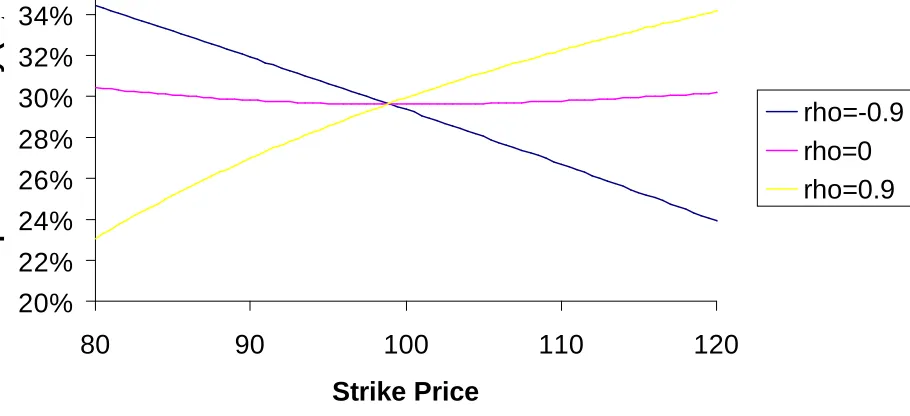
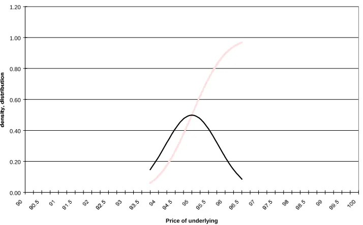
(5) to (13). Figures 1 and 2 show the effect of changing

ρ

on the terminal asset price distribution and

on the volatility smile for options generated under this model with current and long run volatility of

30%, mean reversion

κ

=2 and volatility of volatility

σ

v

of 40%. We can see that the Heston model can

(42)

Figure 1: Implied RNDs Under Alternative

Correlation Parameters

0.0%

0.2%

0.4%

0.6%

0.8%

1.0%

1.2%

1.4%

1.6%

1.8%

50 60

70 80 90 100 110 120 130 140 150 160

Terminal Asset Price

Probability

[image:42.648.103.558.500.708.2]

Rho = -0.9

Rho = 0

Rho = 0.9

Figure 2: Volatility Smile Under Alternative

Correlation Parameters

20%

22%

24%

26%

28%

30%

32%

34%

80

90

100

110

120 Strike Price

Implied Volatility (%)

(43)

An additional feature of the real world that we want to incorporate is the existence of errors that are

the result of discrete tick size intervals (and possibly any small violations of arbitrage within the

settlement prices used for estimation). We want our estimation methodology to be robust to these

small errors in the prices. So we perform the following test of the two RND estimation techniques.

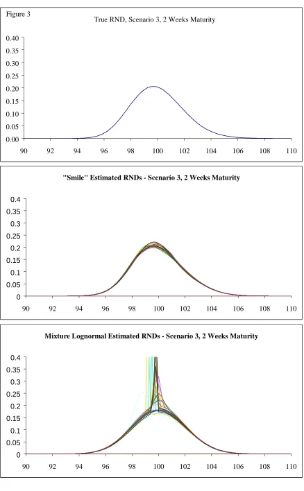
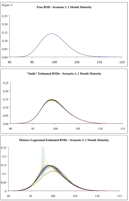
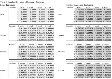
We first establish a set of six scenarios corresponding to low and high volatility and three levels of

skewness. For each scenario we generate a set of options prices with strikes ranging from 30% out-of

the-money to 40% in-the-money. Then for each combination of scenario and maturity we use the

approach developed by Bliss and Panigirtzoglou (1999) to first shock each price by a random number

uniformly distributed from -1/2 to +1/2 a “tick size”. This tick size was chosen as 0.05 to reflect the

sorts of tick sizes that are typically found for exchange-traded options. Given these shocked prices we

fit RNDs using the two techniques described in section two and calculate the summary statistics. We

repeat this procedure of shocking the prices and then fitting the RNDs 100 times for each scenario and

maturity combination. Finally we calculate in each case the mean and standard deviation of the

calculated summary statistics and the squared pricing errors. In essense, this technique simply amounts

to a monte carlo test of the finite sample properties of the two estimators of the sort that is commonly

used within standard econometrics - see Greene (1997) Ch.5 or Davidson and McKinnon (1993) Ch.

18. We then assess the two techniques by comparing the mean estimated summary statistics with the true

summary statistic. We are looking for a technique that has both mean estimates of the statistics that

are close to the true ones and one that has small standard deviations for the calculated statistics in the

presence of the small errors within the options prices used i.e. it is stable. We also want an estimation

procedure that performs well across the range of scenarios and maturities. The next section performs

these tests for European-style options.

4. Results

(44)

differing levels of skewness in the terminal asset price distributions, we use three different levels of the

correlation parameter -0.9, 0 and 0.9. The long run volatilities of 30% for the high volatility scenarios

were chosen on the basis of the levels of implied volatility typically seen within equity markets. The

low volatility (10%) scenarios can be thought of as consistent with levels often seen within FX and

interest rate markets

7

.

Table 1: Model parameters used under each scenario

Strong Negative Skew

Strong Positive Skew

Low Volatility

Scenario 1

κ

=2,

θ

2

=0.1,

σ

v

=0.1,

ρ

=-0.9

Scenario 2

κ

=2,

θ

2

=0.1,

σ

v

=0.1,

ρ

=0

Scenario 3

κ

=2,

θ

2

=0.1,

σ

v

=0.1,

ρ

=0.9

High Volatility

Scenario 4

κ

=2,

θ

2

=0.3,

σ

v

=0.4,

ρ

=-0.9

Scenario 5

κ

=2,

θ

2

=0.3

σ

v

=0.4,

ρ

=0

Scenario 6

κ

=2,

θ

2

=0.3,

σ

v

=0.4,

ρ

=0.9

We test the performance of the two estimation techniques under each of these scenarios across four

different maturities - 2 weeks, 1 month, 3 months and 6 months. For each scenario and maturity

pairing we first generate the true RND and calculate their summary statistics - their mean, standard

deviation, skewness (the third central moment) and kurtosis (the fourth central moment). Table 2 sets

out the true summary statistics for all the maturity and scenario combinations.

7

(45)

[image:45.648.75.401.73.527.2]

Table 2: True Summary Statistics

Scenario 2 weeks 1 month 3 month 6 month 1 100.000 100.000 100.000 100.000 2 100.000 100.000 100.000 100.000

Mean 3 100.000 100.000 100.000 100.000

4 100.000 99.999 99.999 99.994 5 99.999 100.000 99.999 99.998

6 99.988 99.997 99.995 99.961

Scenario 2 weeks 1 month 3 month 6 month

1 1.958 2.878 4.956 6.966

2 1.962 2.888 5.004 7.081

Std Dev 3 1.965 2.898 5.052 7.201

4 5.849 8.555 14.524 20.099

5 5.888 8.677 15.093 21.485

6 5.921 8.799 15.687 22.900

Scenario 2 weeks 1 month 3 month 6 month 1 -0.198 -0.280 -0.418 -0.474

2 0.060 0.089 0.159 0.231

Skewness 3 0.318 0.459 0.743 0.956

4 -0.166 -0.228 -0.301 -0.265

5 0.180 0.272 0.504 0.756

6 0.523 0.776 1.346 1.840

Scenario 2 weeks 1 month 3 month 6 month

1 3.037 3.081 3.178 3.221

2 3.038 3.086 3.221 3.355

Kurtosis 3 3.160 3.344 3.930 4.599

4 2.984 2.962 2.878 2.748

5 3.119 3.269 3.809 4.616

6 3.426 4.036 6.272 9.026

For all combinations the futures price has been set at 100, so the true mean of the distributions are

equal to 100

8

. As we would expect, the standard deviation of the true RNDs increases with maturity

and as volatility is increased. Scenarios 1 and 4 which have a negative correlation between the

underlying asset price and volatility display negative skewness in the terminal asset price distribution.

Except for scenario four

9

, the kurtosis of the terminal asset price distribution is greater than three and

increases with maturity.

8

The slight differences from 100 are caused by error in the numerical integration used to calculate the summary statistics.

9

(46)