Wave scattering from a rough surface: Solution by an iterative method

Wave scattering from a rough surface: Solution

by an iterative method

Guy Tsabary

a

, Yehuda Agnon

b,*

a

Department of Mathematics, Technion, Haifa 32000, Israel

b

Department of Civil and Environmental Engineering, Technion, Haifa 32000, Israel

Received 26 April 2006; received in revised form 27 March 2007; accepted 28 March 2007 Available online 25 April 2007

Abstract

Two iterative solutions of the Helmholtz equation for a scalar field inR3above a rough surface that admits the Dirichlet boundary condition are derived. The bases for the two iterative methods are two different boundary integral equations that represent the solution. The first integral equation is classified as a Fredholm integral equation of the first kind. The second is classified as a Fredholm integral equation of the second kind. This classification suggests that it is easier to find stable solution methods to the second equation. In both methods, the boundary integral was separated into a major part which is easy to calculate and a local residual part. The major part is a convolution and thus can be calculated using FFT in com-plexity O(NlogN), whereNis the number of surface points in which the surface height and its first derivatives together with the incoming wave and its normal derivative are all known. The residual element of the equations can be approxi-mated efficiently only for surfaces where their amplitude is less than the wavelength of the incoming wave. The iterative schemes were tested numerically against a reference solution in order to examine the applicability range, the error estima-tion and the stability of the schemes. All tests supported the superiority of the second method. In particular the error esti-mation and stability tests indicated good performance for surfaces with slope up to 1. Yet, being an equation in the scattered field alone, makes the first method useful as a benchmark solution in its domain of applicability.

2007 Elsevier B.V. All rights reserved.

Keywords: Rough surface; Scattering; Helmholtz equation; Fast Fourier transform; Three-dimensional; Dirichlet to Neumann

1. Introduction

The subject of rough surface scattering has been studied by many methods. Extensive surveys are given in

[44,12]. This paper applies two numerical iterative schemes, each developed from an integral equation

formu-lated for scattering of scalar waves from rough surfaces, subject to a Dirichlet boundary condition. This cor-responds to physical problems such as scattering of acoustic waves from an acoustically soft surface or scattering of electromagnetic waves from a perfect conductor in homogeneous media, where the vectorial formulation of electromagnetic waves can be decomposed into scalar formulations.

0165-2125/$ - see front matter 2007 Elsevier B.V. All rights reserved. doi:10.1016/j.wavemoti.2007.03.006

* _{Corresponding author.}

E-mail address:[email protected](Y. Agnon).

These methods could be classified asSmall slopes methodsin the sense that the surface slope should be less than unity.

The highest efficiency is achieved in the region jSj6_{0:1 minf1;} 1

kAg where Ais the surface amplitude:

A= 0.5(max{g}min{g}) and k is the wave number modulus: k¼

ffiffiffiffiffiffiffiffiffiffiffiffiffiffiffiffiffiffiffiffiffiffiffiffiffiffiffiffiffi kx_i2þky_i2þkz_i2 q

. Beyond this region the complexity increases somewhat: The multiplication factor implied by O(NlogN) is increased from few FFT evaluations to dozens or few hundreds FFT evaluations in the conducted test cases.

The range of validity of the methods presented here exceeds the range of high frequency methods such as Geometrical Optics[17]and[3, pp. 13–21]andKirchhoff approximation[18,23]. They compare favorably other methods such asSmall Slope approximation [16,23] and[43, p. 69],Perturbation expansion [3,20]and more recently[33],Composite-scale[9,38,42,9],Operator expansion[29,30,7] andRayleigh Fano[40,14].

When compared with its closer relatives namely the numerical methods described by Warnick [44, p. 11]

and on, it exhibits better complexity than the Method of moments[39,24] as well as other iterative methods

[27,28,21,11,45].

Perhaps the closest relative numerical methods, are FFT methods. The basic idea is to utilize the high efficiency of the FFT algorithm in performing convolutions, thus reducing the complexity from O(N2) to O(NlogN). The Sparse-Matrix Canonical-Grid (SMCG) method was developed by Li et al. [26,2,46]. The scattering matrix is split into a strong part that consists of near-neighbor interactions and a weak part that consists of all the rest. An iterative scheme such as the conjugate gradient method is adopted to solve the matrix equation. The strong matrix is sparse and can be easily handled. However, the weak interactions require the multiplication of the dense weak matrix with successive iterations and could therefore present a major computational bottleneck. To speed up such calculations, the concept of canonical grid (CG) is intro-duced. The essential nature of CG is that it is translation invariant. In rough surface scattering problems, the CG is usually taken to be the mean flat surface. By translating the unknowns to the CG, the weak interactions can be performed simultaneously for all unknowns using FFT. This reduces memory requirements from O(N2) to O(N) and operation counts from O(N2) to O(NlogN).

The Adaptive Integral method(AIM) [4,1,32] separates near and far field interactions when evaluating a matrix-vector multiplication. To compute far-field interactions, sources supported by the scatterer are pro-jected onto a regular grid by matching their multipole moments (up to a certain order) to guarantee the approximate equality of their far fields. Next, the fields at other grid locations produced by these grid-pro-jected fields are evaluated by a convolution. Knowledge of these fields permits the computation of fields on the scatterer through interpolation. The projection and interpolation operators are represented by sparse matrices, while the convolution can be calculated using an FFT. Unfortunately, the near fields radiated by these grid fields do not match those radiated by the original sources. Therefore, near-field interactions are eval-uated directly, and corrected for errors introduced by the far-field operator.

The Precorrected-FFT method (P-FFT) was introduced by Phillips and White [36,34,35,31]. It further improves the performance of AIM by making the appropriate transformation back from the computational mesh to the physical panels. These methods are most powerful in solving volume scattering problems.

In the present method, a residual equation is established in order to treat the local (near-zone) interactions. This approach clarifies to what extent the near-zone interactions are really local and how good the far-zone operator approximates the integral operator. Thus, it enables a development of far-zone approximations which renders the remainder term increasingly local. Moreover, validity and applicability conditions are straightforward to conclude.

Our approach follows that of[6,13]who used it to solve Laplace’s equation in a water wave problem. Here their approach is extended to solving the case of three-dimensional the Helmholtz equation for rough surface scattering.

1.1. Formulation of the scattering problem

The following notation is adopted: Arrows denote vectors (e.g.~r) and capital letters to denote matrices (e.g. A). The subscript i, s, andgare related to the incident wave (e.g.~ki), the scattered wave (e.g.~ks); and to the rough surface (e.g.~kg), respectively.

Consider the three-dimensional scalar wave functionWð~r;tÞ that satisfies the scalar homogeneous wave equation:

c2r2o 2

ot2

Wð~r;tÞ ¼0

above a rough surface.~r¼ ðx;y;zÞ,cis the wave propagation velocity and$2is the Laplacian.

With the usual separation of variables process, we look for solutions with harmonic time dependence:

Wð~r;tÞ ¼Uð~rÞeixt_:

Let the incident wave be a plane wave:Uið~rÞ ¼eiðk

x

ixþk

y

iyþk

z

izÞ

From now on Uð~rÞ(or rather its normal derivative) is our main concern. This spatial part satisfies the homogenous Helmholtz equation,

ðr2þk2ÞU¼0

and we term it either the wave or the field.

It is assumed that a plane wave is incident from above, upon a rough surfaceoD. The mean location of the surface is atz= 0. The cartesian coordinates (x,y,z) are chosen such thatxandyare horizontal coordinates (spanning the mean surface) andzis upward directed vertical coordinate (normal to the mean surface). The surface (i.e the total reflector boundary) height is represented by a continuously differentiable functiong(x,y) and imposes the Dirichlet BC (Boundary Condition)Ui(x,y,g) =Us(x,y,g) onoD

The mathematical problem to be solved is:

Problem 1. Find a complex valued functionUs(x,y,z) that is

(1) Twice differentiable above the rough surfaceoD.

(2) Satisfies Dirichlet BC:Us=UiwhereUiis a solution of the Helmholtz equation. (3) Us satisfies Sommerfeld radiation condition in the far zone:

limz!1x oUs

ox þy

oUs

oy þz

oUs

oz ikrUs¼0;

The existence and uniqueness of such a solution is proved, for example by Colton[8], Section 3.

The basic tool we use are integral representation theorems.

In the problem with Dirichlet boundary conditions, we may first determine the surface values of the normal derivative of the scattered field,oUs

on. Here, o

on¼~nr~F with~nthe outward unit normal andr~F the gradient of

F. This can be accomplished from the knowledge ofUsvalues that are determined by the Dirichlet BC. There-fore the following equation is a Fredholm integral equation of the first kind:

The uniqueUsthat solveproblem 1, satisfy on the surface

Us 2 ð~rÞ ¼

Z

oD oG

on0ð~r~r 0_ÞU

sð~r0Þ Gð~r~r0Þ

oUs

on0ð~r 0_Þ

ds0 8~r2oD; ð1Þ

whereGðx;y;zÞ ¼ eik ffiffiffiffiffiffiffiffiffiffiffiffi

x2þy2þz2

p

4ppffiffiffiffiffiffiffiffiffiffiffiffiffiffix2_þy2_þz2 is the free space Green’s function for the Helmholtz equation and ds

0_{is the}

dif-ferential area element.

A second kind Fredholm equation can be developed with the additional requirement that restrict the inci-dent wave to be a plain wave, see[19, pp. 1121–1123].

1 2

oU onð~rÞ ¼

oUi

on ð~rÞ Z

oD oG

onð~r~r

0_ÞoU on0ð~r

0_Þds0 _{8~r2oD: ð2Þ}

In the following two Sections 2, 3we develop the iterative schemes for solving Eqs. (1) and (2), respec-tively. These are the main results of this paper. Thereafter in Section 4.1 we develop numerical tests to determine the methods’ stability in the presence of noise and the schemes’ expected error. In Section 5

we develop a similar method to determine the cross-section of the scattered field. Section6 outline the tests that were run in our Matlab programs (to be found in [41]), together with representative results. Conclu-sions are in Section 7.

2. Fredholm equation of the first kind

In this section we introduce the iterative scheme for solving Eq.(1). It is a Fredholm equation of the first kind which is known to be ill conditioned[10, Chapters 12–13],[19, p. 1122]and[5]. Nevertheless, by trans-ferring the equations to the frequency domain, we could avoid the matrix inversion and hence improve con-vergence and stability of our scheme. Although the results in Section 6 indicate the superiority of our 2nd method (based on Eq.(2)), there is at least one significant advantage in solving this equation: It is an equation in Us and its normal derivative alone. This makes it useful for obtaining benchmark solutions.

ConsiderNgrid points on the rough surface. In solving scattering with a Dirichlet BC, the unknown in solving Eq.(1)is the scattered wave normal derivativeoUs

on on the surface. ItsNvalues should therefore be

cal-culated from the knowledge ofUs,g,o_og_x,o_og_yat theNgrid points on the surface. Following Clamond et al.[6], we reformulate Eq. (1)using the following symbols:

(1) Primed variables are used in integrals.

(2)~R¼ ðx;yÞis the two-dimensional projection of~ron the xy-plane. (3) rh~g¼ ðog

ox; og

oyÞ, is the horizontal gradient ofg.

(4) N~¼ ðog ox;

og

oy;1Þ ¼~n

ffiffiffiffiffiffiffiffiffiffiffiffiffiffiffiffiffiffiffiffiffiffiffiffiffiffiffiffiffiffiffiffiffi 1þ ðog

oxÞ

2

þ ðog oyÞ

2 q

denotes a (non-unit) outward normal vector.

(5) o

oN ¼

o on

ffiffiffiffiffiffiffiffiffiffiffiffiffiffiffiffiffiffiffiffiffiffiffiffiffiffiffiffiffiffiffiffiffi 1þ ðog

oxÞ

2

þ ðog oyÞ

2 q

¼ og ox o

ox

og oy o oyþ

o

og, is directional differentiation with respect to~N.

(6) Vs¼o_oU_Ns,Vi¼o_oU_Ni. For simplicity,Vswill replaceo_oU_ns as the unknown in the equation.

(7) r¼ j~r~r0_{j ¼} ffiffiffiffiffiffiffiffiffiffiffiffiffiffiffiffiffiffiffiffiffiffiffiffiffiffiffiffiffiffiffiffiffiffiffiffiffiffiffiffiffiffiffiffiffiffiffiffiffiffiffiffiffiffiffiffiffiffiffiffiffiffiffi_ðxx0_Þ2_{þ ðyy}0_Þ2_{þ ðgg}0_Þ2

q

and R¼ j~_R~_R0_{j ¼} ffiffiffiffiffiffiffiffiffiffiffiffiffiffiffiffiffiffiffiffiffiffiffiffiffiffiffiffiffiffiffiffiffiffiffiffiffiffiffiffi_ðxx0_Þ2_{þ ðyy}0_Þ2

q

are the dis-tances between two 3D and 2D points, respectively.

(8) Gð~r~r0_{Þ ¼}eikr

4pris the Green’s function.

(9) S¼gð~RÞgðR~0_Þ

j~RR~0_j is the slope between two points on the surface. Note thatr¼R

ffiffiffiffiffiffiffiffiffiffiffiffiffi 1þS2 p

.

The reformulation of Eq. (1)is thus:

1 2p

Z Z

oDxy

V0_seikR

R dx

0_dy0_{¼ U}

sþ

1 2p

Z Z

oDxy

4pgoG oN0U

0

sdx0dy0þ

1 2p

Z Z

oDxy

4p oG oN0

goG

oN0 !

U0

sdx0dy0

1

2p

Z Z

oDxy

V0_seikR

R

eikRðpffiffiffiffiffiffiffiffi1þS2_1Þ

ð1þS2Þ12

1

" #

dx0dy0: ð3Þ

Notice that this reformulation illustrates the idea of the method: Addition and subtraction of the boundary

integrals with integrand terms foG oN0,

V0 seikR

R . These are nonlocal terms that are, nevertheless, easy to calculate. On

the other handðoG

oN0f_oo_NG0Þand½e ikRð ffiffiffiffiffiffi1þS2

p

1Þ

ð1þS2Þ12

1are local residual terms, that can either be ignored or reduced to a

smaller linear system. We shall see that if jSj 1 foG

oN0 and

V0seikR

R dominate oG

oN0 and

V0seikr

r , respectively, and the

To constructfoG

oN0, notice that G has the following power series expansion in S:

4pG¼ e

ikRpffiffiffiffiffiffiffiffi1þS2

Rpffiffiffiffiffiffiffiffiffiffiffiffiffi1þS2

e

ikR

R XM

m¼0

amSm¼

XM

m¼0 eikR

Rmþ1 Xm

n¼0

amngng0 mn

;

wherefoG

oN0 is defined by:

4poG oN0

XM

m¼0

og 0

ox0 o eikR

Rmþ1

ox0 og0 oy0

o eikR

Rmþ1

oy0

0 @

1 AXm

n¼0

amngng0 mn

þS e

ikRpffiffiffiffiffiffiffiffi1þS2 R2_ð1þS2

Þ32

ik e ikRpffiffiffiffiffiffiffiffi1þS2 Rð1þS2Þ

!

XM

m¼0

r0hðg 0_{Þ r}0

h

eikR

Rmþ1

_Xm

n¼0

amngng0 mn

þ e

ikR

R2 XM

m¼0

cmSmþ1ik

eikR

R XM

m¼0 bmSmþ1

!

¼ X

M

m¼0

r0 hðg

0_{Þ r}0 h

eikR

Rmþ1

_Xm

n¼0

amngng0 mn

þX

M

m¼0 eikR

Rmþ3 Xm

n¼0

cmnðgnþ

1

g0mngn_g0mnþ1

Þ

ikX

M

m¼0 eikR

Rmþ2 Xm

n¼0

bmnðgnþ

1

g0mngn_g0mnþ1

Þ 4pgoG

oN0; ð4Þ

whereMis preferably chosen small in order to avoid round off error, since in the above analysis we expressed the bounded variableSmas a quotient of two variablesSm_¼ðgg0_Þm

Rm . These vanish at (x0,y0) = (x,y) and

there-after insert big terms such as 1

q2

z,amn.

In what follows we restrict ourselves to the caseM= 0 andS< 1 all over the boundary so that the Tailor series expansion is an adequate choice in the above definition offoG

oN0. With this choicea00=b00=c00= 1 and all the other coefficients vanish so we have:

4pgoG oN0¼

og0 ox0

oeikR

R ox0

og0 oy0

oeikR

R oy0 þ

eikR

R3 ðgg

0_{Þ ik}eikR

R2 ðgg

0_{Þ: ð5Þ}

Eq. (3) and the preceding details suggests a natural decomposition of Vs into three terms Vs¼Vs1þVs2þVs3:

1 2p

Z Z

oDxy

V0_s 1e

ikR

R dx

0_dy0_{¼ U}

sþ

1 2p

Z Z

oDxy

4pgoG oN0U

0

sdx

0_dy0_{; ð6Þ}

1 2p

Z Z

oDxy

V0_s 2e

ikR

R dx

0_dy0_¼ 1

2p

Z Z

oDxy

4p oG oN0

goG

oN0

!

U0_sdx0dy0; ð7Þ

1 2p

Z Z

oDxy

V0_s 3e

ikR

R dx

0_dy0_¼ 1

2p

Z Z

oDxy

V0_seikR

R

eikRðpffiffiffiffiffiffiffiffi1þS2_1Þ

ð1þS2Þ12

1

" #

dx0dy0: ð8Þ

Here Vs1 is the dominant term of Vs, Vs2 is the local contribution and Vs3 is the residual term which is defined implicitly hence calculated iteratively.

Vs1,Vs2andVs3are all approximated by applying FFT on their defining equations. We then make use of the approximate convolution theorem:

Leth(x0_,y0_{) be a periodic function inoD}

xyandg(xx0,yy0) with continuous second derivative such

that its Fourier transform exists, then

1 2p

Z Z

oDxy

gðxx0;yy0Þhðx0;y0Þdx0dy0FFT1f_bgFFTfhgg: ð9Þ

A method to adapt this approximation to the aperiodic nature ofg(xx0_,yy0_{) is outlined at Numerical}

2.1. Calculation of Vs1 (the first order approximation of Vs)

Vs1 is calculated via FFT operation on Eq.(6). Using approximation(9), the left hand side becomes:

FFT 1

2p

Z Z

oDxy

V0_s 1e

ikR

R dx

0_dy0

( )

de

ikR

R FFTfVs1g ¼ i

q_zFFTfVs1g:

Here we used the well known Fourier transform of G: Gbðkx;ky;zÞ ¼ie

izqz

4pqz in the limitz= 0.

In order to approximate the FFT of the right hand integral, one first needs a general equation fordeikR

Rnþ1. This is achieved using the recursion formula

c eikr

rn ¼ i

d

oeikr

rnþ1

ok !

¼ i o

ok deikr

rnþ1 !

;

so that

d eikR

Rnþ1 ¼i Z

lim

r!R

c eikr

rn

! dk¼i

Z _deikR

Rn

! dk:

With the proper integration constants, one gets:

d eikR

R2 ¼i Z _i

q_zdk¼ lnðkþqzÞ; d

eikR

R3 ¼ i Z

lnðkþq_zÞdk¼ iklnðkþq_zÞ þiq_z;

which is sufficient for theM= 0 case.

Now, under the assumption of a common horizontal wavenumber of the surface and the incident wave we can use approximation(9) in the right hand integral of Eq.(6):

FFT 1 2p

Z Z

oDxy

4pgoG

oN0U0sdx0dy0

( )

kx

qz

FFT og 0

ox0U

0

s

ky

qz

FFT og 0

oy0U

0

s

iqzFFTfg0U0sg þigqzFFTfU0sg: ð10Þ

Note that here the relation ondg_oð~_xr~0nr0Þ

m ðkx;kyÞ ¼ ðiÞ

n

kn_mbg was used, which is equivalent to the more standard

relation _oco_xngn

mðkx;kyÞ ¼i

n_kn

mbg, since o

ox0¼ _oðxo_x0_Þ.

The result of this subsection can finally be summarized as:

FFTfVs1g iqzFFTfU 0

sg þikxFFT

og0 ox0U

0

s

þikyFFT og0 oy0U

0

s

q2_zFFTfg0_U0

sg

þq_zFFTfgFFT1fq_zFFTfU0_sggg: ð11Þ

However, the right side is not periodic in kspace, so that Gibbs phenomenon will emerge as soon as we calculateVs1 using FFT

1 .

2.2. Calculation of Vs2 (the second order approximation of Vs)

Similarly, to isolateVs2from(7)we perform FFT on the entire equation, using(9)for the left hand side and limR!0ð

ð~R~R0_Þr0

hg

0

R

gg0

R Þ ¼

R

2

o2_g

iFFTfVs2g qz

¼FFT 1

2p

Z Z

oDxy

eikR gg 0

R3

ð~R~R0_{Þ r}0 hg

0

R3 !

eikRð ffiffiffiffiffiffiffiffi1þS2 p

1Þ

ð1þS2Þ32

1

" #

U0_sdx0dy0

( )

þFFT 1

2p

Z Z

oDxy

ikeikR ð~R~R 0_{Þ r}0

hg 0

R2

gg0

R2 !

eikRð ffiffiffiffiffiffiffiffi1þS2 p

1Þ

ð1þS2Þ 1

" #

U0_sdx0dy0

( )

ð12Þ

FFT 1

2p

Z yþD₂y

yD₂y

Z xþDx

2

xDx

2

eikR 1 2RUsð0Þ

o2g oR2ð0Þ

_eikRðpffiffiffiffiffiffiffiffi1þS2_1Þ

ð1þS2Þ32

1

" #

dx0dy0 (

þ 1

2p

Z yD₂y

yAy

þ

Z yþAy

yþD₂y

! Z xþAx

xAx

þ

Z yþD₂y

yD₂y

Z xDx

2

xAx

þ

Z xþAx

xþDx

2 !

" #

eikR

R2

gg0

R

ð~_R~_R0_{Þ r}0 hg

0

R !

eikRðpffiffiffiffiffiffiffiffi1þS2_1Þ

ð1þS2Þ32

1

" #

U0_sdx0dy0 )

ð13Þ

FFT 1

2p

Z yþD₂y

yD₂y

Z xþDx

2

xDx

2

ikeikR 1

2Usð0Þ

o2g oR2ð0Þ

eikRðpffiffiffiffiffiffiffiffi1þS2_1Þ 1þS2 1

" #

dx0dy0 (

þ 1

2p

Z yD₂y

yAy

þ

Z yþAy

yþD₂y

! Z xþAx

xAx

þ

Z yþD₂y

yD₂y

Z xDx

2

xAx

þ

Z xþAx

xþDx

2 !

" #

ikeikR

R

ð~_R~_R0_{Þ r}0 hg

0

R

gg0

R !

eikRðpffiffiffiffiffiffiffiffi1þS2_1Þ 1þS2 1

" #

U0_sdx0dy0 )

; ð14Þ

whereAxandAyare chosen as small as possible thus utilizing the locality ofð_oo_NG0f_oo_NG0Þ. Later in this chapter we will show how to choose them adequately. Integrals(13) and (14)were separated according to their singu-larity. Following Macaskill and Kachoyan in[27, Appendix A], one can show that integral(12)can be approx-imated at first order as:

Z yþD₂y

yD₂y

Z xþDx

2

xDx

2

eikR 1

2RUsð0Þ

o2g oR2ð0Þ

eikRðpffiffiffiffiffiffiffiffi1þS2_1Þ

ð1þS2_Þ32

1

" #

dx0_dy0_I1

13ðq1Þ I113ðQ1Þ þI213ðq1Þ I213ðQ1Þ; ð15Þ

where

I1₁₃ðFÞ ¼

Z Dy

Dx

Dy

Dx

Usð0Þsin kDxF

2

_g

xxþv21gyyþ2v1gxy

kF4 dv1;

and

I2₁₃ðFÞ ¼

Z Dx

Dy

Dx

Dy

Usð0Þsin kDyF

2

_v2

2gxxþgyyþ2v2gxy

kF4 dv2;

with

v1¼y

x; q1ðv1Þ ¼

ffiffiffiffiffiffiffiffiffiffiffiffiffiffiffiffiffiffiffiffiffiffiffiffiffiffiffiffiffiffiffiffiffiffiffiffiffiffiffiffiffiffiffiffiffiffiffiffiffiffiffiffiffiffiffiffiffiffiffiffiffiffiffi

ð1þg2

xÞ þv

2

1ð1þg2yÞ þ2v1gxgy

q

; Q₁ðv1Þ ¼

ffiffiffiffiffiffiffiffiffiffiffiffiffi 1þv2 1 q

;

v2¼x

y; q2ðv2Þ ¼

ffiffiffiffiffiffiffiffiffiffiffiffiffiffiffiffiffiffiffiffiffiffiffiffiffiffiffiffiffiffiffiffiffiffiffiffiffiffiffiffiffiffiffiffiffiffiffiffiffiffiffiffiffiffiffiffiffiffiffiffiffiffiffi

ð1þg2

yÞ þv22ð1þg2xÞ þ2v2gxgy

q

; Q₂ðv2Þ ¼

ffiffiffiffiffiffiffiffiffiffiffiffiffi 1þv2 2 q

:

Similarly, the first order approximation of integral(14)yields:

Z yþDy

2

yD2y

Z xþDx

2

xDx

2

ikeikR 1

2Usð0Þ

o2g

oR2ð0Þ

eikRðpffiffiffiffiffiffiffiffi1þS2_1Þ

1þS2 1

" #

dx0dy0I1

where

I1₁₄ðFÞ ¼

Z Dy

Dx

DDyx

Usð0Þ 1 kF sin

kDxF 2

Dxcos kDxF 2

_g

xxþv21gyyþ2v1gxy

F3 dv1;

and

I2₁₄ðFÞ ¼

Z Dx

Dy

Dx

Dy

Usð0Þ 1 kF sin

kDyF 2

Dycos kDyF 2

_v2

2gxxþgyyþ2v2gxy

F3 dv2:

Having established the way for calculatingVs1 andVs2, let us calculateVs3.

2.3.Vs3 calculation and the total normal derivative Vs

The definition ofVs3 leads to the iterative process. Applying the following steps in the given order defines the iterative scheme:

(1) DefineV0_sN ¼V0_s 1þV

0

s2þV

0N

s3 for eachNP1.

(2) Define the initial values required for the iterative scheme: ForN= 0,V0_s0¼0 and forN= 1V0_s1 3¼0. (3) Apply FFT to Eq.(8).

(4) Subtract theNth iteration from theN+ 1st. (5) Add FFTfV0_s

1þV

0

s2gto both sides.

Then, for eachNP1 one gets,

FFTfV0Nþ1

s g ¼FFTfV

0N

s g þ

iq_z 2pFFT

Z Z

oDxy

eikR_ðV0N

s V

0N1

s Þ

R

eikRðpffiffiffiffiffiffiffiffi1þS2_1Þ

ð1þS2Þ12

1

" #

dx0dy0

( )

FFTfV0N

s g þ

iq_z 2pFFT

Z yþD₂y

yD₂y

Z xþDx

2

xDx

2

eikR_ðV0N

s V

0N1

s Þ

R

eikRð ffiffiffiffiffiffiffiffi1þS2 p

1Þ

ð1þS2Þ12

1

" #

dx0dy0

( )

þiqz

2pFFT

Z yDy

2

yAy

þ

Z yþAy

yþD₂y

! Z xþAx

xAx

þ

Z yþDy

2

yD₂y

Z xDx

2

xAx

þ

Z xþAx

xþDx

2 ! (

eikR_ðV0N

s V0

N1

s Þ

R

eikRðpffiffiffiffiffiffiffiffi1þS2_1Þ

ð1þS2Þ12

1

" #

dx0dy0 )

; ð17Þ

where the singular integral is approximated using the same method as[27, Appendix A]:

Z yþD2y

yDy

2 Z xþDx

2

xDx

2

eikR_ðV0N

s V0

N1

s Þ

R

eikRðpffiffiffiffiffiffiffiffi1þS2_1Þ

ð1þS2Þ12

1

" #

dx0dy0

ðVN

sðx;yÞ V

N1

s ðx;yÞÞ

Z Dy

Dx

DDyx

2 kq2₁sin

kDxq₁ 2

dv1 Z Dy

Dx

DDyx

2 kQ2₁sin

kDxQ₁ 2

dv1

" #

þ ðVN_sðx;yÞ VN_s1ðx;yÞÞ

Z Dy

Dx

D_Dy_x

2 kq2₂ sin

kDyq₂ 2

dv2

Z Dy

Dx

D_Dy_x

2 kQ2₂ sin

kDyQ₂ 2

dv2

" #

: ð18Þ

With the same definitions ofv1,v2,q1,q2,Q1andQ2as used in(15) and (16). Again the minimization ofAx

andAyis crucial in order to minimize the calculation effort in each iteration.

To summarize this subsection, the estimation of the normal derivative isV0N

s . The stopping condition forN is:kjV0sN1

V0N

2.4. Determining adequate Axand Ayfor calculations ofVs2 andVs3

To calculateVs2 we findR

*_{such that for anyR>R}*_,joG

oN0f_oo_NG0j jf_oo_NG0j.

Confining the discussion to the caseM= 0 andS< 1 which we employed above it is easy to show that

4p oG oN0

goG

oN0 !

¼eikR gg

0

R3

ð~R~R0Þ r0hg0

R3

!

eikRðpffiffiffiffiffiffiffiffi1þS2_1Þ

ð1þS2Þ32

1

" #

þikeikR ð~R~R0Þ r 0 hg0

R2

gg0

R2 !

eikRðpffiffiffiffiffiffiffiffi1þS2_1Þ

ð1þS2Þ 1

" #

: ð19Þ

A sufficient condition forjoG

oN0f_oo_NG0j jf_oo_NG0j is:

max

R>R

eikRðpffiffiffiffiffiffiffiffi1þS2_1Þ 1þS2 1

! ; e

ikRðpffiffiffiffiffiffiffiffi1þS2_1Þ

ð1þS2Þ32

1

!

( )

1:

An upper limit forSthat maintains the above inequality is established through the Tailor series expansion

ofpffiffiffiffiffiffiffiffiffiffiffiffiffi1þS2around S = 0 that yields eikRðpffiffiffiffiffiffiffiffi1þS2_1Þ

eikRS22 ¼e ikðgg0Þ2

2R . Thereafter, the expansion of e

ikðgg0 Þ2

2R around

ikðgg0_Þ2

2R ¼0, requires a tighter condition:

jSj min 1; 1 kA

; ð20Þ

Which is then translated to a condition on R,

RmaxfA;A2kg; ð21Þ

whereA¼maxoDxyf

jgg0_j

2 g, is the surface amplitude.

In these conditions eikðgg0Þ 2

2R 1þikðgg

0_Þ2

2R , hence a first order approximation inSyields:

eikRðpffiffiffiffiffiffiffiffi1þS2_1Þ 1þS2 1

!

ikRS2

2 þS

2

1þS2

eikRðpffiffiffiffiffiffiffiffi1þS2_1Þ

ð1þS2Þ32

1

!

ikRS2

2 þ

3S2

2 1þ3S2

2 :

Moreover, since requirement (21)assure the extinction of the above terms, it is a sufficient condition to determineAxandAyforVs2.

The same condition(21)is sufficient forVs3. Typical settings forAx,Aycan be:

Ax¼minfLx;5 maxfA;A2kgg; Ay ¼minfLy;5 maxfA;A2kgg: ð22Þ

Special treatment should be applied to confinexAx,x+Ax,yAyandy+Ayinto the surface edges

bound-ary. As an example consider a rectangular surface [0,Lx]·[0,Ly], then the integral RxþAx

xAx

RyþAy

yAy is translated as:

Z xþAx

xAx

Z yþAy

yAy

Z minfLx;xþAxg

maxf0;xAxg

Z minfLy;yþAyg

maxf0;yAyg

: ð23Þ

Three remarks concerning conditions(20) and (21)will close this section:

• These conditions imply that our method is efficient at surfaces such that max {A,A2k}max {Lx,Ly}. In

this respect it is a low frequency or small amplitude method.

• Higher order expansions of foG

oN0 might improve condition(21).

• The highest slope in sinusoidal surfaces isA

ffiffiffiffiffiffiffiffiffiffiffiffiffiffiffiffiffi kx_g2þky_g2 q

3. Fredholm equation of the second kind

In this subsection we introduce the iterative scheme for solving Eq.(2). It is a Fredholm equation of the second kind which is known to be well conditioned. This is the reason for its superior performance compared to the first method. Following the procedure of the previous section, multiplication by 2 of Eq.(2)followed by addition and subtraction of the dominant integrals produces the analogous of Eq.(3):

Vsþ 1 2p

Z Z

oDxy

V0_s4pofG oNdx

0_dy0_¼V

i

1 2p

Z Z

oDxy

V0_i4pofG oNdx

0_dy0 _ð24Þ

1

2p

Z Z

oDxy

ðV0_iþV0_sÞ4p oG oN

f

oG

oN !

dx0dy0: ð25Þ

We abbreviate the integrals in Eqs.(24) and (25)by

VsþIs24¼ViIi24I25:

In contrast to the first equation, the calculation of Vs is based here on the values ofVi(rather than Ui). AgainoeG

oN is considered the dominant part of oG

oN and is easily calculated. oG

oN e

oG

oN is considered as a local residual

part. BothV0_ioeG oN,V

0

se

oG

oN are added and subtracted to the original equation for efficient calculation. Since the

pro-cedure in this equation is almost identical with the first propro-cedure, the details can be skipped. One difference worth noting is that here the differentiation is with respect to the unprimed variables. This enters sign

differ-ences compared to the differentiation in the previous section equation. In particular oeG

oN 6¼f

oG

oN0 and the Fourier

transform of the derivatives become the regular one: cong oxn

ið

kx;kyÞ ¼inknibg.

For theM= 0 and maxoDjSj< 1 (assumed from now on), an application of approximation(9)to integral Is

24 yields:

Is₂₄iFFT1fq_zFFTfg0V0_sgg þog oxFFT

1 kx

q_zFFTfV

0

sg

þog oyFFT

1 ky

q_zFFTfV

0

sg

igFFT1fq_zFFTfV0_sgg: ð26Þ

The same is true for integralIi

24so we can build an iterative scheme that ignores the residual integral(25)in Eq. (24).

The initial estimations forVsare based on the dominance ofo_oeG_N. Thereafter, theNth iteration is subtracted from the (N+ 1)th iteration. This way, we get the following iterative scheme:

f Vs0¼Vi

f

Vs1¼Vi2iFFT1fqzFFTfg0V0igg 2

og oxFFT

1 kx

q_zFFTfV

0

ig

2og

oyFFT

1 ky

q_zFFTfV

0

ig

þ2igFFT1fq_zFFTfV0_igg

f

VsNþ1¼fVsN iFFT1 qzFFT g 0 f_V0

s

N f_V0

s

N1

n o

n o

og oxFFT

1 kx

q_zFFTfðfV

0

s

N f_V0

s

N1_Þg

og oyFFT

1 ky

q_zFFTfðVf

0

s

Nf_V0

s

N1_Þg

þigFFT1 q_zFFTfðfV0_sN _Vf0

s

N1_Þg

n o

Again FFT1is applied to aperiodic terms so that Gibbs phenomenon will surely emerge. In addition, pow-ers ofqzappear in the the denominator of some terms, accordingly we will have to eliminate these terms

arti-ficially in the neighborhood ofqz= 0 to avoid singularity inaccuracies.

A sufficient condition for the extinction ofI25is:jo_oG_NooeG_Nj j_ooeG_Nj

Otherwise we use the settle point of this scheme as a starting point to the iterative scheme of the exact equation:

V0

s¼fVsN1 V1s ¼VfsN

VN_sþ1¼VN_s iFFT1fq_zFFTfg0ðV0_sN V0_sN1Þgg

og oxFFT

1 kx

q_zFFTfðV

0N

s V0

N1

s Þg

og oyFFT

1 ky

q_zFFTfðV

0N

s V0

N1

s Þg

þigFFT1 _q

zFFTfðV0 N

s V0

N1

s Þg

1

2p

Z Z

oDxy

ðV0_sNV_s0N1Þ4p oG oN

f

oG

oN !

dx0dy0: ð28Þ

The last integral in the above scheme, is treated by the method applied to the right hand of Eq.(13). The next section discusses stability and error estimations.

4. Stability and error estimations

We chose to detect the validity (definiteness) of the methods described at Sections2 and 3by inspecting the solutions sensitivity to noise: the stability, and by estimating the error in absence of known analytic solution.

4.1. Stability

The linear algebra theory, suggests the investigation of maximal eigenvalues of the relevant matrix as the natural tool to investigate the system’s stability. Anyhow our matrix size (AN·N, such thatN=NxÆNyP104)

does not afford completion of such investigation which is at least O(N2) complex (see e.g., the power method in

[15]). An alternative (feasible) way is ad-hoc investigation of the sensitivity ofV~s against ‘‘small’’ changes of eitherV~ior in the integral operator. The former investigation is the more widely used one and we adopt it as well.

For the first scheme, we first apply incoming waveU1i and sign our scheme solution for it byVf 1

s. Then we add small noiseeU2

i with normal derivativeeV 2

i such thatjeU 2

ij jU

1

ij8ðx;yÞ 2oDxy. Thus this time we apply

U3_i ¼U1_i þeU2_i to the scheme and sign its scheme solution byVf3_s. Trivially we define the stability as:

StabilityEðjVf

1

s Vf

3

sjÞ

EðjeV2

ijÞ

; ð29Þ

whereE(Æ) is the boundary mean.

For the second scheme one needs to apply some normal derivativeV1_i, sign its solution scheme by Vf1_s. Thereafter apply a disturbed waveV3_i ¼V1_i þeV2_i such thatjeV2_ij jV1_ij 8ðx;yÞ 2oDxyto the scheme and

eval-uate the stability.

Clearly, ifStability1 then the scheme is stable. On the other hand, if StabilityP2 it is sensitive to mea-surement noise.

4.2. Error estimation of Section3

dEðjVsfVsjÞwithout the need inVs(which we usually do not know). To do so, we reuse fVs in order to

solve the original equation for Vfi. The quotientEðj_EV_ðji_VVeijÞ

ijÞ , will serve us an upper bound to the average relative errorEðjVsVesjÞ

EðjVijÞ .

Indeed, no prove is supplied to approve thatEðjVifVijÞ>EðjVsVfsjÞ. Nevertheless, the asymmetry of the two iterative processes suggests that the errors in the two stages will accumulate rather than subtract. Hence we will solve now Eq.(2) forfVi:

f

Viðx;y;gðx;yÞÞ ¼Vfsðx;y;gðx;yÞÞ þ2 Z Z

oDxy

ðfV0_sþfV0_iÞoG oN dx

0_dy0_{; ð30Þ}

Following Section3 and with the same definitions, we transform the equation into its deflated form:

f Vi

1 2p

Z Z

oDxy

f V0_i4pofG

oNdx

0_dy0_¼fV

sþ

1 2p

Z Z

oDxy

f V0_s4pofG

oNdx

0_dy0 _ð31Þ

þ 1

2p

Z Z

oDxy

ðfV0_iþfV0_sÞ4p oG oN

f

oG

oN !

dx0dy0: ð32Þ

Again we restrict our attention to the special caseM= 0 andS< 1. Starting with the truncated equation (that does not include the residual integralI32) one gets:

e Vi;0¼Ves

e

Vi;1¼Vesþ2iFFT1 qzFFTfg0Ve0sg

n o

þ2og

oxFFT

1 kx

q_zFFTfVe

0

sg

þ2og

oyFFT

1 ky

q_zFFTfVe

0

sg

2igFFT1nq_zFFTfVe0_sgo

e

Vi;nþ1¼Vei;nþiFFT1 qzFFTfg0ðVe0i;nVe 0

i;n1Þg

n o

þog oxFFT

1 kx

q_zFFTfðVe

0

i;nVe

0

i;n1Þg

þog oyFFT

1 ky

q_zFFTfðVe

0

i;nVe0i;n1Þg

igFFT1 _q

zFFTfðVe0i;nVe 0

i;n1Þg

n o

: ð33Þ

As in scheme(28), in surfaces that does not satisfy requirement(20)almost everywhere, the last terms of the above iterative scheme will serve as initial guess for the accurate equation scheme:

e

Vi;0¼Vei;n1 Vei;1¼Vei;n

e

Vi;nþ1¼Vei;nþiFFT1fqzFFTfg0ðVe0i;nVe 0

i;n1Þgg

þog oxFFT

1 kx

q_zFFTfðVe

0

i;nVe

0

i;n1Þg

þog oyFFT

1 ky

q_zFFTfðVe

0

i;nVe

0

i;n1Þg

igFFT1fq_zFFTfðVe0_i;nVe0_i;n1Þgg

þ 1

2p

Z Z

oDxy

ðVe0_i;nVe0_i;n1Þ4p oG oN

f

oG

oN !

dx0dy0; ð34Þ

4.3. Error estimation of Section2

Here the quotientEðjUseUsjÞ

EðjUsjÞ , will serve as an upper bound to the average relative error

EðjVsVesjÞ

EðjVijÞ . Note that this quotient differs from the one supplied to the second schemeðEðjViVeijÞ

EðjVijÞ Þ, since the solution of Eq.(1)will not equip us withfVi. The amplification or suppression inspired by the replacement ofEðjVsfVsjÞ withEðjUsUesjÞis cancelled by the division operation which replaceViwithUs.

Indeed, no prove is supplied to approve that this is an upper bound, yet, the asymmetry of the two iterative processes suggests that the errors in the two stages will accumulate rather than subtract. Hence we will solve now Eq. (1) for Ues. Following Section 2 and with the same definitions, we transform the equation into its deflated form:

e

Us

1 2p

Z Z

oDxy

4pgoG oN0Ue

0

sdx

0_dy0 1

2p

Z Z

oDxy

4p oG oN0

goG

oN0 !

e

U0_sdx0dy0

¼ 1

2p

Z Z

oDxy

f Vs0eikR

R dx

0_dy0 1

2p

Z Z

oDxy

f Vs0eikR

R

eikRðpffiffiffiffiffiffiffiffi1þS2_1Þ

ð1þS2Þ12

1

" #

dx0dy0: ð35Þ

This time we chose to follow the reasoning of Section 3 with M= 0 andS< 1. If maxjSj minf1;1

kAg

almost everywhere then we can approximate the accurate equation by:

e

Us

1 2p

Z Z

oDxy

4pgoG oN0Ue

0

sdx

0_dy0 1

2p

Z Z

oDxy

f Vs0eikR

R dx

0_dy0_;

for which we can develop cheap iterative scheme (O(NlogN)):

e

Us;0¼ iFFT1

FFTffVsg q_z

( )

e

Us;1¼Ues;0FFT1 kx

q_zFFT

og0 ox0Ue

0

s;0

FFT1 ky q_zFFT

og0 oy0Ue

0

s;0

iFFT1nq_zFFTfg0Ue0_s;0goþgfVs

e

Us;nþ1¼Ues;nFFT1

kx

q_zFFT

og0 ox0ðUe

0

s;nUe

0

s;n1Þ

FFT1 ky q_zFFT

og0 oy0ðUe

0

s;nUe

0

s;n1Þ

iFFT1fq_zFFTfg0ðUe0_s;nUe0_s;n1Þgg þigFFT1nq_zFFTfUe0_s;nUe0_s;n1go: ð36Þ

Otherwise, the last terms of the above iterative scheme will serve as initial guess for the accurate equation scheme:

e

Us;0¼Ues;n1 Ues;1¼Ues;n

e

Us;nþ1¼Ues;nFFT1

kx

q_zFFT

og0 ox0ðUe

0

s;nUe

0

s;n1Þ

FFT1 ky q_zFFT

og0 oy0ðUe

0

s;nUe

0

s;n1Þ

iFFT1fq_zFFTfg0ðUe0_s;nUe0_s;n1Þgg þigFFT1fq_zFFTfUe_s0_;nUe0_s;n1gg

þ 1

2p

Z Z

oDxy

4p oG oN0

goG

oN0 !

ðUe0_s;nUe0_s;n1Þdx0dy0; ð37Þ

where the last boundary integral is truncated in the same way as in Section2.4.

5. Calculation of the scattered field above the surface

Usð~rÞ ¼ Z

oD oG

on0ð~r~r 0_ÞU

sð~r0Þ Gð~r~r0Þ

oUs

on0ð~r 0_Þ

ds0; ð38Þ

For a detailed proof one can refer to [8] page 69 and on. As opposed to Eq. (1), in this equation the unknown term isUs. It is a Fredholm equation of the second kind, thus it should be stable. Since this equation differs from(1) only by a factor, the solution will be similar. The natural substitute to R is:

Ra

ffiffiffiffiffiffiffiffiffiffiffiffiffiffiffiffiffiffiffiffiffiffiffiffiffiffiffiffiffiffiffiffiffiffiffiffiffiffiffiffiffiffiffiffiffiffiffiffiffi

ðxx0_Þ2_{þ ðyy}0_Þ2_þz2 q

:

where the subscript a stands for above. The natural replacement toSis:

Sa

ffiffiffiffiffiffiffiffiffiffiffiffiffiffiffiffiffiffiffiffiffiffiffiffiffiffiffiffiffiffiffiffiffiffiffiffiffiffiffiffiffiffi

g2_ðx0_;y0_{Þ 2zgðx}0_;y0_Þ

p

Ra

¼

ffiffiffiffiffiffiffiffiffiffiffiffiffiffiffiffiffiffiffi

g02_2zg0

p

Ra

:

As in the surface definitions

r

ffiffiffiffiffiffiffiffiffiffiffiffiffiffiffiffiffiffiffiffiffiffiffiffiffiffiffiffiffiffiffiffiffiffiffiffiffiffiffiffiffiffiffiffiffiffiffiffiffiffiffiffiffiffiffiffiffiffiffiffiffiffi

ðxx0_Þ2_{þ ðyy}0_Þ2_{þ ðzg}0_Þ2

q

¼Ra

ffiffiffiffiffiffiffiffiffiffiffiffiffi 1þS2_a q

:

Note that any unprimed variable is located strictly above the surface. With these notations we can rewrite Eq. (38)in its deflated form:

2Usðx;y;zÞ ¼ 1 2p

Z Z

oDxy

4pgoG oN0U

0

sdx

0_dy0

1

2p

Z Z

oDxy

V0_seikRa

Ra

dx0dy0 ð39Þ

þ 1

2p

Z Z

oDxy

4p oG oN0

goG

oN0 !

U0_sdx0_dy0 1

2p

Z Z

oDxy

V0_seikRa

Ra

eikRað

ffiffiffiffiffiffiffiffi

1þS2

a

p 1Þ

ð1þS2_aÞ12

1

" #

dx0_dy0 _ð40Þ

This time foG

oN0 is expended in powers of Sa. The discussion is restricted to M= 0, and to z>A so that jSaj< 1. Applying FFT to the entire equation yields:

2FFTfUsg ¼

ieizqz

q_z FFTfV 0

sg þF:T e

ikRa_ðxx0_Þ 1

R3_a ik R2_a

FFT og 0

ox0U

0

s

þF:T eikRa_ðyy0_Þ 1

R3 a ik R2 a

FFT og 0

oy0U

0

s

þF:T e

ikRa

R3

a

ike

ikRa

R2

a

FFT ðg0zÞU0s

ð41Þ

1

2pFFT Z Z

oDxy

eikRa gg

0

R3

a

ð~R~R

0_{Þ r}0

hg

0

R3

a

! eikRað

ffiffiffiffiffiffiffiffi

1þS2

a

p

1Þ

ð1þS2_aÞ32

1

" #

U0

sdx

0_dy0

( )

ð42Þ

þ 1

2pFFT Z Z

oDxy

ikeikRa gg

0

R2

a

ð~R~R

0_{Þ r}0

hg

0

R2

a

!

eikRað ffiffiffiffiffiffiffiffi1þS2

a

p

1Þ

ð1þS2

aÞ 1

" #

U0

sdx

0_dy0

( )

ð43Þ

1

2pFFT Z Z

oDxy

V0_seikRa

Ra

eikRað

ffiffiffiffiffiffiffiffi

1þS2

a

p

1Þ

ð1þS2_aÞ12

1

" #

dx0dy0

( )

¼ ie

izqz

q_z FFTfV 0

sg

kxe

izqz

q_z FFT

og0

ox0U

0

s

kye

izqz

q_z FFT

og0

oy0U

0

s

þe

izqz

z FFTfðg 0_zÞU0

sg þFFTfI42þI43þI44g; ð44Þ

where the symbolF.T{f} replaces the previousbf due to the lengthy nature of the transformed terms. The

mul-tiplier term FFTfðg0_zÞU0

sg results from the equality

eikRa

R3

a

ikeikRa

R2

a ¼

oeikRa Ra

oðz2_Þ.I42, I43and I44 can all be trun-cated according to the methods outlined at Section 2.4. Furthermore, we can totaly eliminate them at points for which zmax {A,A2k} which assure that Saminf1;kA1g.

6. Numerical tests and results

is eitherVsor FFT{Vs}. The results are demonstrated using graphs. These substantially differ from the pop-ular Bistatic Coefficient graphs (as used by[24–26,21,22]and more). We will explain this choice later on. The chosen reference solution is the one of Macaskill and Kachoyan in[27]. We chose it due to its resemblance to our second method and its dependance on the same Eq.(2). Macaskill et al. solve this equation by simple iter-ation method in O(N2) which restricted its application size to N= 104 net size (for moderate computer resources).

The following five tests were conducted:

6.1. Test 1: Basic comparison

In cases where the first method could be considered accurate, we used the following strategy: For the first method, we can feed a known solution of Eq.(1)such as plane wave propagating in the positive direction of the z axis:

Usðx;y;zÞ ¼eijk

x

sjxþijk

y

sjyþijkzsjz ) _V

s¼ ijkxsj

og oxijk

y

sj

og oyþijk

z

sj

Us:

The input isUsand the output should be the accurate (known)Vs. Yet since the scheme solution,fVs, differs fromVs, We denote the difference by:e1stðx;yÞ ¼ jVsfVsj.

e1stcan now serve us as good estimate to the error of the scheme when solved for the dual incoming wave. That is the same wave but with a propagating direction opposite to thez-axis:

Uiðx;y;zÞ ¼eijk

x

sjxþijkysjyijkzsjz _{) V}

i¼ ijkxsj

og oxijk

y

sj

og oyijk

z

sj

Ui:

If we denote the exact (unknown) solution of the scattering problem ofUibyVsand the numerical solution byVe1st

s we can estimate that:

jVe1st_s j6_{jVsj je}1st_j:

With this estimation under hand, we can estimate the errors inVe2nd

s andVeMacs which are the numerical solu-tions of our second scheme and the one of Macaskill, respectively:

If for example jVe1st

s Ve2nds j6je1stj, then the two methods are consistent. Otherwise, we can confidently conclude that the second method’s error is greater than ±e1st. As a working method, this test is recommended as a calibration tool rather than an applicability test due to its narrow applicability range (up to slopes of 0.1). For this reason we demonstrate its performance with as simple parameter values as possible. We applied this test to the Laplace equation (k= 0) as well by cautious changes in the relevant programs. The results of the Laplace equation case were far better than the ones performed for the Helmholtz equation and enabled work-ing with slopes of 0.5.

The representative cases presented are:

(1) The number of surface points for a wavenumber (sampling rate) must exceed the Nyquist Rate (2 points per cycle). We set the minimal rate to 4 in our programs. Hence,Nx(the total number of net points along

thex-axis), must comply with

NxPMinRatemax

Lx kx_i;

Lx kx_g

( )

¼LxMinRatemaxfk x

i;k

x gg

2p :

Similarly,Ny(the total number of grid points along they-axis), must comply with

Ny PMinRatemax

Ly ky_i;

Ly ky_g

( )

¼LyMinRatemaxfk y

i;k

y gg

In practice, the parameters settings work flow is as follows:

(a) The number of net points along each axis (NxandNy) were set in advance.

(b) The surface lengthesLxandLyare then set in a way that assure the minimal sampling rate of the

incoming wave as well.

(c) The values ofkx_gandky_galways obeyed both the minimal sampling rate and the conditionskxg

kx

i 2 Qand

kyg

ky_i 2Q. The last conditions reduce the FFT Gibbs phenomenon.

(2) Both the incoming wave and the surface were chosen so that the y-axis wavenumber was zero. This way, our solutions could be compared with one-dimensional solvers solutions.

(3) Size parameters:Nx= 128,Ny= 4.

(4) Waves parameters:

Usðx;y;zÞ ¼eik

x

ixþik

y

iyþik

z

iz; U_iðx;y;zÞ ¼eikxixþik

y

iyik

z

iz

k¼2p; h¼45; /¼0; k_ix¼ksinðhÞcosð/Þ ¼ppffiffiffi2;

ky_i ¼ksinðhÞsinð/Þ ¼0; kz_i ¼kcosðhÞ ¼ppffiffiffi2:

(5) Surface parameters:

0 50

—50

—100 100

0 50

—50

—1000 100

0.2 0.4 0.6 0.8 1

kx

0 0.002 0.004 0.006 0.008 0.01

kx

0 50

—50

—100 100

kx

0 0.02 0.04 0.06 0.08

a

b

c

d

—100 —50 0 50 100

—150 —100 —50 0 50

kx

Bistatic Coefficient (dB)

[image:16.544.76.470.70.405.2]

1st Method 2nd Method

Lx ¼

8 ffiffiffi 2

p ; Ly ¼1; A¼0:045; kxg¼ p

ffiffiffi 2

p ; ky_g¼0;

Slope¼A

ffiffiffiffiffiffiffiffiffiffiffiffiffiffiffiffiffi kx2

g þk y2

g

q

¼0:1; gðx;yÞ ¼Asinðkx gxþk

y gyÞ:

Following the stated policy of determining the accuracy of the first solution it was found on average 1% accurate.

FromFig. 1(c) and (d) it is seen that Macaskill’s method results are inconsistent with our two methods. On

the other hand, our two methods are found to be mutually consistent in the sense that their difference graph

(Fig. 1(c)) has the same scale as the error estimation (1%).

To explain this inconsistency we developed the next test.

6.2. Test 2: Treatment of compact (aperiodic) roughness

Examination of our schemes and Macaskill’s scheme uncover a substantial difference in the basic assumptions that lead to the schemes: The usage of cyclic convolution in our schemes suggests that if the scheme rectangle rep-resent a small part of cyclic ‘‘infinite’’ boundary (as may occur in ocean surfaces) then our schemes are the ade-quate tool to solve the scattering problem. If on the other hand the region of roughness has a compact support, then Macaskill’s method is the adequate tool. Yet we can use zero padding policy in order to approach the com-pact support case. The more zero padding we use, the better the expected agreement. The essence of the second test is therefore applying zero padding tog,UsandVi. We applied an increasing region of zeroes to the same case and tested the error between our second method and Macaskill’s. Test parameters:

(1) Determination of the test case scales and net points, see test6.1number 1.

(2) The multiplication factors of the basic grid point numbersNx,Nywhere chosen to ben= {1, 2, 4, 8, 16}

so as to preserve the power of 2 nature ofNxandNy. Thus, the spacial vectorsx, ywere enlarged to

x= [0:(nNx1)]dxandy= [0:(nNy1)]dy.The arrays ofViandgand its derivatives were zero padded adequately. For example, for each nP2,g(Nx+ 1:nNx, 1:nNy) = 0 and g(1:Nx, Ny+ 1:nNy) = 0.The

frequency plane entitieskx,ky,qzwere refined. For example, for eachnP2,kx¼_nL2p_x½nN₂x:nN₂x1.

(3) Basic size parameters:Nx= 64,Ny= 32.

(4) Incoming wave parameters:Uiðx;y;zÞ ¼eik

x

ixþik

y

iyik

z

iz where

k¼2p; h¼45; /¼30; kx_i ¼ksinðhÞcosð/Þ ¼p

ffiffiffi 3 2 r

;

ky_i ¼ksinðhÞsinð/Þ ¼ p_ffiffiffi

2

p ; kz_i¼kcosðhÞ ¼ppffiffiffi2:

(5) Surface parameters:

Lx ¼4

ffiffiffi 2 3 r

; Ly¼2

ffiffiffi 2

p

; A¼0:0225;

p

ffiffiffi 3 2 r

6kx g6

17ppffiffiffi3

8 ; k

y g¼

p

ffiffiffi 2

p ; Slope¼A

ffiffiffiffiffiffiffiffiffiffiffiffiffiffiffiffiffi kx2

g þk y2

g

q

¼0:1;

gðx;yÞ ¼cAsinðkx gxþk

y gyÞ þ

cA 4 sinð2k

x gxþ3k

y gyÞ þ

cA 9 sinð7k

x gxþ4k

y gyÞ;

where the constantcthat multipliesAmakes sure that the slope do not exceed 0.1.

6.3. Test 3: Error estimation

Notice the relative instability around Hi= 35; we chose to limit the investigation to the range 106_Hi6_{80out of which the stability performance deteriorates.}

The parameters of this test are:

(1) Determination of the test case scales and grid points, see test6.1number 1. (2) Size parameters:Nx= 32,Ny= 64.

(3) Incoming wave parameters:h ranges from 15to 85rather than a single value. Aside from this all the details coincide with those of test6.2number 3.

(4) Surface parameters: Replace in test6.2number 4Lx ¼2p_kx

i, Ly ¼4p_ky

i

andkx_g/2p

Lx,k

y g/

2p

Ly. These settings are

in accord with the changes inkx_i andky_i above.

6.4. Test 4: Stability

This test applies the stability test as described in Section4.1for both the first and the second methods. The calculation was performed over various values of kx_g and hi and then calculated the stability as defined by definition(29). The figures in this test presents the dependence of the stability onkx_gandhiat various slopes. The other parameter settings are equal to the ones in test6.3. For the slope of 0.5 2nd method we excluded

Hi= 35which did not converge.

6.5. Test 5: Performance

Here we conducted a large scale test that proves the capabilities of the schemes. The large rough surface were set bumpy enough to cause the costly procedures 17 and 28 to become active. As reference we investi-gated slopes for which only the inexpensive approximations are active. The test parameters are:

(1) Determination of the test case scales and grid points see test6.1number 1. (2) Size parameters:Nx= 1024,Ny= 256.

(3) Incoming wave parameters: Replaceh value withh= 20in test 6.2number 3. (4) Surface parameters: SetLx= 108.03, Ly= 46.78, A= 0.26,

kx_g¼1:92; ky_g¼0:13; Slope¼A

ffiffiffiffiffiffiffiffiffiffiffiffiffiffiffiffiffi kx_g2þky_g2 q

¼0:5

and put the appropriate c in Section6.2number 4. A slope of 0.1 achieved by decreasing of A served as a reference test where the expensive schemes 17 and 28 are inactive.

7. Discussion

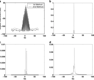
The Bistatic CoefficientFig. 1(a) demonstrates the weakness of the Bistatic (logarithmic) measure: It is easy to notice that the error is hard to discern exactly in the most interesting direction (where dominant scattering intensity occurs) and is emphasized in the unimportant directions, where scattering is negligible. This property distorts the error graph in a way that convinced us to look for an alternative presentation: Normalization of they-axis scale to the maximal scattering intensity.

As mentioned in subsection 6.1 the average error was preliminary investigated by solving Eq. (1) with the dual outgoing plane wave. Thus, we could treat the first method solution in this test as accurate to 1%.

In Fig. 1(b) the incoming wave direction is set to its correct direction (i.e. into the rough surface). This

figure illustrates the scattering intensity as a function of thex-axis wave numberkx. The connection between

hs¼Arctan

ffiffiffiffiffiffiffiffiffiffiffiffiffiffiffiffiffiffiffiffiffiffiffiffiffi k2k2_xk2_y

k2_xþk2_y v

u u t 0 @

1 A:

As expected, the maximal intensity direction is the specular refraction direction kx= 4.44. The figure is

plotted for ky= 0 since any other direction contained negligible intensities due to its non specular nature.

Enlargement of the minimal sampling rate from 4 to 8 (see additional details in Section6.1) reduced the error by approximately a factor 2, whereas additional refinements of the minimal rate show no improvement.

The error graph 1(c), demonstrates agreement between our two methods. In contrast graph 1(d) demon-strates inconsistency between Macaskill’s Method and ours. As is evident from the results of the next test, this inconsistency can be ascribed to the compact rough surface assumption of Macaskill et al. versus our periodic rough surface assumption.

As a closing remark to this test let us mention that we applied this test to Laplace equation (k= 0) with superior results that allowed the tests to be considered successful up to slopes of 0.5.

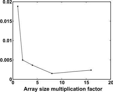
Fig. 2illustrates the maximal error (y-axis) between our second method and Macaskill’s as a function of the

arrays size multiplication factor 1,2,4,8,16 (x-axis). The left hand value of this graph is approximately 0.02 which is consistent with the results demonstrated at graph 1(d). The trend is for better agreement with more zero padding. Furthermore the maximal error received with this factor is approximately 0.003 which is within the error range predicted by test6.1.

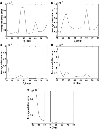
Fig. 3(a)–(e), demonstrate the dependence of the average error (defined at Section4.1) on both the anglehi

(the angle between the incoming wave number vector and thez-axis) and thex-axis surface wavenumberkx_g. The first two graphs 3(b) and 3(a), show the relative error at slopeS(g) = 0.1. Comparing them reveals the supreme performance of the second test with respect to the average error estimation. Yet, comparison of these results with those of test 6.1 suggests that we cannot consider the relative error to be an upper bound to the ‘‘real’’ error between the numerical and theoretical solutions. One possible explanation to this is that the numerical schemes settle points differs substantially from the theoretical settle point. Consequently we recommend to treat this error test as an upper bound of the applicability range. With this in mind,

Fig. 3(d) provides an upper slope threshold of 0.5 to the first method. Fig. 3(e) shows an upper threshold

of slope 1 to the second method.

Let us also mention that for 06_hi6_{10 and 80}6_hi6_{90 the results become divergent. Consequently,} 106_hi6_{80 is the application range for our method.}

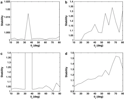
Fig. 4demonstrates the stability, as defined at(29), as a function of the anglehiand the surfacex-axis

wave-numberkx

g. Graphs 4(b) and 4(a), are for slope up toS(g) = 0.1. They reveal that both methods are stable at

this slope, with the second method performing better. The other couple of graphs are the methods stability performance for surfaces with slopes up to 0.5. Again the second method performs better. Our last test was a performance test. The computation time was a few seconds for the small slopes approaching S(g)6_0.1

0 5 10 15 20

0 0.005 0.01 0.015 0.02

[image:19.544.180.369.516.669.2]

Array size multiplication factor

where only the inexpensive steps of the schemes were involved. The computation time was a few hours for the higher slopes where the heavy calculation steps become active. For the time consuming cases the second method was twice as fast as the first one so that the superiority of the second method is evident in computation cost as well.

10 20 30 40 50 60 70 80

0 0.2 0.4 0.6 0.8

1x 10

—7

θ_i (deg)

Average relative error

10 20 30 40 50 60 70 80

0 0.2 0.4 0.6 0.8 1 1.2 1.4x 10

—7

θ_i (deg)

Average relative error

10 20 30 40 50 60 70 80

0 0.2 0.4 0.6 0.8

1x 10

—6

θ_i (deg)

Average relative error

10 20 30 40 50 60 70 80

3 3.5 4 4.5 5 5.5

6x 10

—3

θ_i (deg)

Average relative error

10 20 30 40 50 60 70 80

0 0.5 1 1.5

2x 10

—6

θ_i (deg)

[image:20.544.71.471.63.580.2]

Average relative error

8. Conclusions

(1) The first method is recommended as a benchmark solution with a good estimation on its error size for mild slope surfaces (S6_0.1).

(2) Otherwise, the conducted numerical tests, suggest the usage of the second method as the default choice. For this reason it is the default subject of the below listed conclusions.

(3) Numerical behavior is satisfactory to slopes of at least 1. This is the conclusion from tests6.3 and 6.4. (4) Test6.3reveals the angle range 106_hi6_{80 that the method can be applied to.}

(5) The characteristic complexity for small slopes surfacesðjSj6_{0:1 minf1;} 1

kAgÞis O(NlogN) dominated

by few FFT evaluations. The memory consumption is O(N). This makes the iterative method attractive. (6) In steeper surfaces the complexity is multiplied by factorCM. Eventually,CMis the number of iterations (few) times the number operations required to evaluate the local residual integrals. Thus,CMis propor-tional to the number of net points in the region [xAx,x+Ax]·[yAy,y+Ay] whereAx= min {Lx,

5 max {A,A2k}} andAy= min {Ly, 5max {A,A2k}}. Consequently,Low frequencyorSmall amplitude

surfaces are more efficiently handled.

(7) No complications are predicted in extending our methods the Neumann BCðoUsðx;y;gðx;yÞÞ

on ¼

oUiðx;y;gðx;yÞÞ

on Þ.

Here the unknown term of the direct scattering problem becomesUs. Eq. (1) is therefore a Fredholm equation of the second kind and thus predicted to supply steady and reliable solutions. Eq.(2), should be replaced by:

10 20 30 40 50 60 70 80

1 1.005 1.01 1.015 1.02 1.025

θ_i (deg) θ

i (deg)

θ_i (deg)

θ_i (deg)

Stability

10 20 30 40 50 60 70 80

1 1.05 1.1 1.15 1.2 1.25 1.3 1.35 1.4

Stability

10 20 30 40 50 60 70 80

1 1.05 1.1 1.15 1.2 1.25 1.3 1.35 1.4

Stability

10 20 30 40 50 60 70 80

0.9 1 1.1 1.2 1.3 1.4 1.5 1.6

[image:21.544.66.481.67.396.2]

Stability