An adjusted location model for SuperDARN backscatter echoes

(1)

Ann. Geophys., 30, 1769–1779, 2012 www.ann-geophys.net/30/1769/2012/ doi:10.5194/angeo-30-1769-2012

Annales

Geophysicae

An adjusted location model for SuperDARN backscatter echoes

E. X. Liu1,2, H. Q. Hu2, R. Y. Liu2, Z. S. Wu1, and M. Lester3 1_{School of Science, Xidian University, Xi’an 710071, China}

2_{State Oceanic Administration Key Laboratory for Polar Science, Polar Research Institute of China, Shanghai 200136, China} 3_{Department of Physics and Astronomy, University of Leicester, Leicester LE1 7RH, UK}

Correspondence to: E. X. Liu (liuerxiao@pric.gov.cn)

Received: 1 August 2012 – Revised: 2 November 2012 – Accepted: 2 December 2012 – Published: 21 December 2012

Abstract. The radars that form the Super Dual Auroral Radar Network (SuperDARN) receive scatter from ionospheric ir-regularities in both the E- and F-regions, as well as the Earth’s surface, either ground or sea. For ionospheric scat-ter, the current SuperDARN standard software considers a straight-line propagation from the radar to the scattering zone with an altitude assigned by a standard height model. The knowledge of the group delay to a scatter volume is not suf-ficient for an exact determination of the location of the irreg-ularities. In this study, the difference between the locations of the backscatter echoes determined by SuperDARN stan-dard software and by ray tracing has been evaluated, using the ionosonde data collected at Sodankyl¨a, which is in the field-of-view of Hankasalmi SuperDARN radar. By studying elevation angle information of backscattered echoes from the data sets of Hankasalmi radar in 2008, we have proposed an adjusted fitting location model determined by slant range and elevation angle. To test the reliability of the adjusted model, an independent data set is selected in 2009. The result shows that the difference between the adjusted model and the ray tracing is significantly reduced and the adjusted model could provide a more accurate location for backscatter targets. Keywords. Ionosphere (Ionospheric irregularities) – Radio science (Radio wave propagation)

1 Introduction

The Super Dual Auroral Radar Network (SuperDARN) (Greenwald et al., 1995; Chisham et al., 2007) is a network of ground-based coherent scatter radars that operate in the HF band and whose field-of-view combines to cover extensive regions of both the Northern and Southern Hemispheres’ po-lar, auroral and mid-latitude ionospheres. SuperDARN forms

a powerful tool for monitoring ionospheric and magneto-spheric dynamics and it has been successful in addressing a wide range of scientific questions concerning processes in the magnetosphere, ionosphere, thermosphere, and mesosphere, as well as general plasma physics (Chisham et al., 2007). In contrast to UHF and VHF radio waves, high frequency (HF) radio waves are very susceptible to refractive effects. The or-thogonality condition can be achieved between the wave vec-tor and the Earth’s magnetic field for the SuperDARN HF radars by the refraction of radio waves in the ionosphere. To produce coherent backscatter, the irregularity separation along the radar beam must be half of the radio wave length. For HF radars this corresponds to a separation of between 7.5 m and 18.75 m. These irregularities are produced by some processes, such as the gradient drift and the two-stream in-stability mechanisms (Jones et al., 2001; Fejer and Kelley, 1980). According to Bates and Albee (1970), the maximum backscatter power is produced when the wave vector direc-tion is perpendicular to the Earth’s magnetic field lines (i.e. perpendicular to the irregularities aligned with the magnetic field lines). At HF, the refractive effects of the ionosphere en-sure that the field line orthogonality condition can be satisfied in the ionosphere over a very large area.

When the radio waves propagate through the ionosphere, they will refract and some of them can achieve the orthog-onality condition to the Earth’s magnetic field lines. Such waves have a chance to be backscattered if the ionospheric irregularities of proper size exist at the ranges of orthogo-nality. Currently, the location of the HF returns is generally determined by a simple range-finding algorithm, which as-sumes straight line propagation at the speed of light from the radar site to a target at a given altitude above the Earth, and thus takes no direct account of the prevailing HF prop-agation conditions (Yeoman et al., 2001) and the elevation

(2)

1770 E. X. Liu et al.: An adjusted location model for SuperDARN backscatter echoes

angle information is not used. The standard model used to determine the locations of the irregularities for SuperDARN ionospheric backscatter is:

h1(r)=

      

115r

150 0< r <150 km

115 150≤r≤600 km

r−600

200 ·(hi−115)+115 600< r≤800 km

hi r≥800 km

(1)

g1(r)=REcos−1

"

R2_E+(RE+h1(r))2−r2 2RE(RE+h1(r))

#

(2)

whereREis the radius of the Earth,r is the slang range (in km),h1(r)is the virtual height (in km),g1(r)is the ground range (in km),hi is a user-defined virtual height (in km), which is typically taken as 300 km or 400 km.

A number of previous studies have attempted to assess the accuracy of the SuperDARN algorithm and the associated SuperDARN location model. These studies have sometimes adopted a ray tracing simulation approach to assess the ac-curacy of the range-finding algorithm (Villain et al., 1984), or have used velocity cross-correlation between signals from the same radar at different frequencies (Andre et al., 1997). Yeoman et al. (2001) made use of artificially induced iono-spheric irregularities and the ray tracing simulation to test the SuperDARN algorithm, and suggested that typical ground range errors were of∼16 km for 1₂-hop F-region backscat-ter and ∼60 km for 11₂-hop F-region backscatter. Yeoman et al. (2008) demonstrated that the typical ground range er-rors were larger than this and that the standard SuperDARN virtual height model was inadequate for accurately mapping scattering locations at far ranges.

In fact, the altitude from which the backscatter originates can be estimated from a knowledge of the range to the backscatter volume (i.e. slant range), and a measurement of the elevation angles of the radar returns, determined using the interferometric technique described by Milan et al. (1997a). Without detailed knowledge of the electron density profile, straight-line propagation must be assumed. The elevation angle 1, radar slant range r, the altitude h2(r, 1) and the ground rangeg2(r, 1)of the scatter volume are then related by

h2(r, 1)=(R_E2+2RErsin1+r2)1/2−RE (3)

g2(r, 1)=REsin−1

_r_cos₁

RE+h2(r, 1)

(4) However, this assumption is reliable for the determination of altitude in the lower ionosphere and at shorter ranges (Milan et al., 2001). Errors may become significant for longer paths

where the curvature of the Earth becomes important (Yeo-man et al., 2008). Furthermore, it is generally understood that the assumption of a fixed height for F-region SuperDARN echoes and a specific choice of 400 km or 300 km are both seldom correct, though the errors involved are typically not significant (Andre et al., 1997).

In this paper, a ray tracing simulation has been performed for 119 time intervals from 2008, during which there is clear scatter from ionospheric irregularities received by the Hankasalmi SuperDARN radar. The electron density used for ray tracing is from the ionosonde data collected at So-dankyl¨a, which is located in beam 9 of the Hankasalmi field-of-view at a distance of∼650 km to the radar site. By com-bining backscattered signals’ elevation angles information from the data set and ray tracing simulation, we first es-timate the possible real height of ionospheric echoes, and then the ground difference between the results from the stan-dard SuperDARN software and ray tracing. By fitting a low-order polynomial (linear and quadratic, respectively) to the height and ground range data, we propose an adjusted loca-tion model determined by slant range and elevaloca-tion angle, based on the analysis on the radio wave propagation paths. Finally, to test the reliability of the adjusted model, we have chosen an independent data set of 128 time intervals in 2009.

2 Methods and results

In this study we have chosen to use the data from beam 9 of the Hankasalmi SuperDARN radar to estimate the echoes height and obtain the adjusted fitting model. Only common mode data (in which the range from the radar site to the first range gate is 180 km, and the range gate separation is 45 km) are used to simplify the analysis and the method of presenta-tion of the results.

2.1 Hankasalmi SuperDARN radar

(3)

E. X. Liu et al.: An adjusted location model for SuperDARN backscatter echoes 1771

26 / 30

567 Figure 1

568

569 Figure 2

[image:3.595.88.512.61.310.2]

570

Fig. 1. Hankasalmi radar beam 9 echo maps for (a) power, (b) Doppler velocity, (c) width and (d) elevation angles from 23:30 UT on 15 May to 00:30 UT on 16 May 2008. The radar operating frequency was 9.945 MHz.

the European Incoherent Scatter radar (EISCAT) and the ionosonde at Sodankyl¨a (Hankasalmi range of∼650 km).

It is critical to know that Hankasalmi ionospheric echoes received at ranges of less than 900 km quite often come from the E-region, sometimes from the F-region and sometimes from both E- and F-region (Milan et al., 1999, 2001). At far-ther ranges of 900∼1500 km, the echoes are usually from F-region height. All these types of echoes are expected to be received via the 1₂-hop propagation model, i.e. direct radio wave propagation to the scattering area with the appropriate amount of refraction.

Figure 1 illustrates an example of echoes received on beam 9 of the Hankasalmi radar from 23:30 UT on 15 May to 00:30 UT on 16 May 2008 (MLT≈UT+2 h, with a slight difference from∼1.8 h in gate 0 to∼2.3 h in gate 40). From Fig. 1, it can be seen that the main echoes are received from 900 km to 2000 km. Some echoes at closer ranges, i.e. less than 900 km, are classified as ground echoes by the stan-dard SuperDARN software because of low velocity (shown in Fig. 1b) and low width (shown in Fig. 1c). It is likely, how-ever, that this scatter has been misidentified as ground scat-ter as the elevation angles indicate that this scatscat-ter is from the same region as the higher velocity scatter. We also note that there is little ground scatter at far ranges. This could be because signal attenuation over a long-distance path is sig-nificant such that the radar cannot detect echoes with too low S/N (signal to noise ratio), or the ionospheric electron density is insufficient to cause enough refraction to result in 1-hop propagation. Figure 1d shows that nearly all echoes have

el-evation angles less than 20◦and most less than 14◦. It is also interesting to note that the elevation angles of the echoes ap-proximately decrease with range except a few echoes at far ranges with very high elevation angles more than 20◦. The cause of the occasional elevation angles above 20◦is uncer-tain and is beyond the area of interest in this study.

2.2 Ray tracing simulation

The HF ray path tracing program used in this study was originally developed by Jones and Stephenson (1975). In the present study we introduce IRI-2007 (Bilitza and Reinisch, 2008) electron density profiles to the ray tracing. We also use the ionosphere parameters foE, foF1 (if present), foF2 and M(3000)F2 measured from the Sodankyl¨a ionosonde data to scale the IRI profile enabling a more realistic calculation to be performed. The partial derivative used in the ray tracing model is calculated by the Richardson extrapolation numer-ical method (Press et al., 2007). For the geomagnetic field modeling, the IGRF model (Macmillan and Maus, 2005) is used.

Figure 2 shows an example of one of the ray tracing results for the centre time of the interval shown in Fig. 1. The hor-izontal axis is the ground range from the radar site, and the vertical axis is the height. The calculation is made for beam 9 of the SuperDARN Hankasalmi radar, as well as paths of var-ious rays in the ionosphere at elevation angles from 1◦ to 29.5◦, spread at every 0.5◦. The thick lines represent the el-evation angles every 5◦, starting at 5◦. In order to observe ionospheric backscatter echoes, it is required that the radar

(4)

26 / 30

567

Figure 1

568

569

Figure 2

570

Fig. 2. Simulated ray path plot. The traces correspond to elevation angles from 1◦to 29.5◦; the rays with elevation angles of 5◦, 10◦, 15◦, 20◦, 25◦are illustrated by thick lines. The green squares plot-ted on the rays indicate that the rays are within 1◦of normality to the Earth’s magnetic field. The green dashed line corresponds to 160 km height. The simulation is done for Hankasalmi radar beam 9.

wave vector is normal to the ambient magnetic field vec-tor (Greenwald et al., 1995). Each green square along a ray trace identifies where the angle between radar HF ray vector and the ambient magnetic field vector is within the range of 90◦±1◦, at which locations ionospheric field-aligned irreg-ularities, if present, would cause scatter of the HF signal.

Figure 2 demonstrates that ray paths with elevation angles greater than 15◦_{penetrate the ionosphere without satisfying}

the perpendicularity criterion. The rays with an elevation an-gle of less than 15◦can achieve the orthogonality condition. This is consistent with the data shown in Fig. 1d (the eleva-tion angle informaeleva-tion) where the maximum elevaeleva-tion angle was 14◦, apart from the unusual and sparse high (≥20◦) val-ues. Figure 2 also demonstrates that the ionospheric echoes can come from quite a large range of altitudes and ground range. There are two distinct regions of potential echoes, provided irregularities exist. One occurs at ranges between 300 km and 1500 km and heights of 70 km and 160 km, while the second occurs between ranges of 900 km and 1900 km and heights of 160 km and 300 km. We can also note that echoes with heights above 180 km can originate at the same range but from two ionospheric heights with significantly dif-ferent elevation angles, which has been discussed in previ-ous studies (Uspensky et al., 1994; Kprevi-oustov et al., 2007). F-region echoes with larger elevation angles occur at shorter ranges (slant range) and correspond to the “connection” part of the top and bottom parts of the F scattering zone. The range dependence of the elevation angle is consistent with actual radar data shown in Fig. 1d.

27 / 30 571

Figure 3

572

573

Figure 4

574

Fig. 3. Height distribution of ionospheric backscatter echoes for the event in Fig. 1. The different color represents the height from ray tracing calculation.

2.3 Echo height estimation

Figure 2 illustrates a mixture of echoes from the ground range between 900 km and 1800 km for this interval. Echoes with the same slant range may come from different heights and correspond to different ranges. By ray tracing with the knowledge of the radar elevation angles, we can estimate more accurate real height and ground location of the echoes. Figure 3 shows the distribution of the real height estimates of ionospheric backscatter echoes for the interval in Fig. 1. The different colors represent the echoes’ real height esti-mates from ray tracing calculation using actual range and el-evation angle data. Echoes with elel-evation angles larger than 15◦are excluded from the ray tracing, because the rays with larger takeoff angles suffer little refraction in the ionosphere and therefore tend not to achieve the orthogonality condition with the Earth’s magnetic field. Figure 3 demonstrates that the real height estimates of possible irregularities vary signif-icantly from 140 km to 300 km in this interval. The average real height estimates of all these points with heights greater than 160 km is 252 km, which was also considered to be the typical height of F-region echoes during this time interval.

Figure 4 presents statistical histograms of echo occurrence for UT, elevation angle, and range gate in the Hankasalmi radar beam 9 data set in 2008 (panels a) and 2009 (pan-els b). The criteria used to select the data are as follows: days with obvious ionospheric echoes in gates less than 40 (∼1980 km, equivalent to 1₂-hop) and duration time are se-lected every month; the 5 days with the lowestP_K

(5)

27 / 30 571

Figure 3 572

573

[image:5.595.309.544.344.507.2]

Figure 4 574

Fig. 4. Statistical histograms of universal time (UT), elevation angle and gate for Hankasalmi beam 9 common mode data in (a) 2008 and (b) 2009.

To ensure a minimal amount of ground backscatter in the calculation, we reject all echoes with a line-of-sight velocity below the velocity threshold of 50 m s−1_{and with a Doppler} width below the level of 50 m s−1. The top panel of Fig. 4a presents the distribution of1₂-hop scatter as a function of UT and MLT, where MLT≈UT+2. From the histogram, there is a significant UT bias in the occurrence in 2008, with a minimum near 06:00 UT and peaks either side of 24:00 UT and post noon. The lack of ionospheric scatter in the 05:00– 10:00 UT sector is consistent with the occurrence of iono-spheric scatter in 1995–1996 (Milan et al., 1997b). The sec-ond panel of Fig. 4a presents the elevation angle histogram. The distribution of elevation angles is determined partly by the vertical radiation pattern formed by the SuperDARN an-tennae, which will peak at a particular elevation angle for a particular operational frequency and beam orientation; the elevation angles of arrival will be the same as the takeoff an-gles, assuming identical propagation paths to and from the scattering region. Here, the histogram peaks around an el-evation angle of 8◦. The range gate distribution has a peak around gate 23 (∼1215 km), which may correspond to high E-region or F-region backscatter. The statistical histograms of the data set in 2009 are very similar to those in 2008, with the major difference being the shift of the peak occurrence in elevation angle to around 10◦, which is slightly larger than that of 2008, as shown in Fig. 4b.

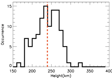
Figure 5 summarizes the statistical distribution of the aver-age height of the 119 intervals from 2008 determined by ray tracing. In any individual interval, we only consider iono-spheric echo altitudes larger than 160 km. From Fig. 5, the maximum occurrence of the intervals occurs between 230 km

28 / 30

575

Figure 5 576

577

Figure 6 578

579

Figure 7 580

Fig. 5. Statistical histograms of average height for a total of 119 intervals in 2008. The red vertical dashed line illustrates 239 km, which is the average height of the 119 intervals.

and 240 km with a mean over the 119 intervals of 239 km in-dicated by the red vertical dashed line. In individual cases, the height can be below 180 km and importantly has a clear difference from the default SuperDARN F-region echo vir-tual height of either 300 km or 400 km.

2.4 Difference between the results from the standard model and ray tracing

Figure 6 summarizes our results of ground difference distri-bution of the total 119 intervals in 2008. In order to avoid the significant statistical discrepancy due to a small amount

(6)

28 / 30

575

Figure 5

576

577

Figure 6

578

579

Figure 7

580

Fig. 6. The standard deviation (green lines) and the mean deviation (red lines) of ground range between the results of standard Super-DARN model and the ray tracing for the data set in 2008.

of data points, the elevation angles of ionospheric echoes are limited between 1◦and 18◦, and between range gate 10 and 40 (equivalent to 630 km and 1980 km).

The red line indicates the mean deviation (md), which rep-resents the difference of the results from the SuperDARN standard model minus the results from ray tracing; the green line indicates the standard deviation (std, the mean square error). The mean deviation of ground difference is in the range from−10 km to 100 km, increasing with range gate, or ground range and is mainly positive, which means the ground range of the standard model is mainly larger than that identi-fied by ray tracing. Therefore, the standard model places the scattering points farther from the radar than those identified by ray tracing. This figure confirms that for the standard Su-perDARN model, in most cases, the backscatter echoes from the lower ionosphere may be misidentified as echoes from the higher ionosphere, i.e. some E-region backscatter is being treated as F-region backscatter, which may lead to the con-tamination of global convection maps. Chisham and Pinnock (2002) presented examples which highlight the importance of identifying the contamination of global convection maps, which results from the addition of non-F-region backscatter. Such contamination can greatly affect mesoscale features of the structure of flow vortices, convection reversal boundaries, and flow transients. Hence, it is crucially important to iden-tify the origin of ionospheric echoes.

2.5 Data fitting and the adjusted new model

Using the observation described above, we can now investi-gate whether they can be used to provide a new model for determining the ground range of ionospheric scatter. We fit a low-order polynomial (both a linear and quadratic form) to the height and ground range data of 119 intervals in 2008, which were calculated by ray tracing using the elevation an-gles and slant range data from SuperDARN data set. The

forms are as follows:

g(r, 1)=A1·r2+B1·r+C1·12+D1·1+E1·r·1+F1 (5)

h(r, 1)=A2·r2+B2·r+C2·12+D2·1+E2·r·1+F2 (6) whereg(r, 1)is the ground range model andh(r, 1)is the real height model determined by slant ranger(unit, km) and elevation angle1(unit, degree). The coefficients of the fit-ting results (A, B, C, D, E, F and R-square) are presented in Table 2. The fitted curves are also shown in Fig. 7: The color lines represent the new model determined by slant range and elevation angle by fitting the data from ray tracing to a lin-ear and a quadratic polynomial, and the black line represents the standard SuperDARN model. The elevation angle infor-mation is also indicated by the color bar at right side with the value from 0◦_{(blue) to 24}◦_{(red). As we know, the real}

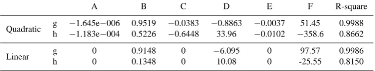
height models differ from the standard virtual height model and the height of the standard model is basically larger than the height of new model based on ray tracing. The coefficient of determination, the R-squared measure of goodness of fit is used to show how well the model fits the data set. The R-square of the height fitting for linear and quadratic fitting are all greater than 0.8, while for the ground range fitting, the R-square is above 0.99.

(7)

[image:7.595.133.458.83.144.2]

Table 1. Geographic and geomagnetic locations of the instrumentations.

Instrument Geographic location Geomagnetic location

Latitude,◦N Longitude,◦E Latitude,◦N Longitude,◦E

Hankasalmi 62.32 26.61 59.78 105.53

Sodankyl¨a 67.37 26.63 64.14 106.59

Table 2. The coefficients of Eqs. (5) and (6).

A B C D E F R-square

Quadratic g −1.645e−006 0.9519 −0.0383 −0.8863 −0.0037 51.45 0.9988 h −1.183e−004 0.5226 −0.6448 33.96 −0.0102 −358.6 0.8662

Linear g 0 0.9148 0 −6.095 0 97.57 0.9986

h 0 0.1348 0 10.08 0 -25.55 0.8150

the height of the new fitting model and that of the ray trac-ing. The standard deviation of height in most gates is less than 20 km and 40 km for quadratic and linear fitting, respec-tively. In particular, the overlap region where scatter can be from either the E-region or F-region, the ground range dif-ference is less than∼10 km and the height difference is less than 25 km. We do note that a larger height difference be-tween the ray tracing and new real height model can occur in some gates, especially for the linear model.

Using the new model also reduces the skew of the ground range difference distribution and moves the centre of the dis-tribution closer to zero ground range difference, with a very small skew present in some gates. Hence, using this new ad-justed model has removed the major deviations in the ground range that clearly existed in Fig. 6, leaving predominantly random and systematic error. In summary, this adjusted new model can provide more accurate basis for our determination of a new location model.

3 Discussion

Determination of the location of SuperDARN HF iono-spheric echoes is a challenging problem. Previous studies have shown that the height of F-region echoes can be very different in different ionosphere environments (Villain et al., 1984; Andre et al., 1997; Milan and Lester, 2001; Yeoman et al., 2001; Danskin et al., 2002; Koustov et al., 2007). Villain et al. (1984) utilized a modified form of three-dimensional ray tracing program by Jones and Stephenson (1975) to es-timate that the typical heights of F-region echoes are more than 300 km. Milan and Lester (2001) showed that the max-ima of occurrence distribution for the altitude identified as F-region backscatter is near 230 km by using Hankasalmi inter-ferometer data from the myopic experimental mode, which concentrates on near ranges in the field of view. Danskin et al. (2002) predicted that the ionospheric echoes are expected

to come from the altitudes of 190∼250 km with elevation angles of between 20◦and 30◦, which is in reasonable agree-ment with radar measureagree-ments. Koustov et al. (2007) used tomographic estimates of the electron density to predict the expected heights of F-region coherent echoes by ray tracing and obtained typical echo heights of 275 km. All the studies mentioned above indicate great variability in the location of ionospheric backscatter.

Andre et al. (1997) used multifrequency HF radar data ob-tained with the SHERPA (Syst`eme HF d’Etude Radar Po-laires et Aurorales) radar to analyze the error introduced on the localization of ionospheric scatters by straight-line prop-agation and constant scattering altitude. With a judicious choice of the scattering altitude, the maximum error can be of the order of 20 km, while changing the scattering altitude by 100 km introduces a difference of only 20 km in range for the localization of the scatter.

An evaluation of the absolute range-finding accuracy of the current routine analysis of SuperDARN data has been performed by Yeoman et al. (2001) using HF radar backscat-ter, which has been artificially induced at a precisely known location by a high-power RF facility (ionospheric heater) operated by the European Incoherent Scatter Scientific As-sociation at Tromso (EISCAT). The ground range location was found to be accurate to within 16 km and 60 km for di-rect 1₂-hop and 11₂-hop backscatter, respectively. The result is perhaps unsurprising because the operating frequency of the radar is 19 MHz and the radio wave propagation through ionosphere is likely to be closer to a straight line propagation than the typical observation frequencies of 10∼12 MHz. Yeoman et al. (2008) demonstrated that the typical ground range errors are larger than this and the standard SuperDARN virtual height model is inadequate for accurately mapping scattering locations at far ranges.

Chisham et al. (2008) evaluated the difference between the ground range from Eqs. (2) and (4) and developed a

[image:7.595.107.487.183.255.2]

(8)

28 / 30

575

Figure 5 576

577

Figure 6 578

579

Figure 7 580

Fig. 7. (a) The height model determined by slant range and elevation angle. The color lines represent new height model of linear and quadratic fitting. The black line represents the standard virtual height model of SuperDARN. (b) The ground range model determined by slant range and elevation angle. The color lines represent new model. The black line represents the standard ground range model of SuperDARN shown in Eq. (4). The scatter points are used for fitting. The color bar indicates the elevation angle information.

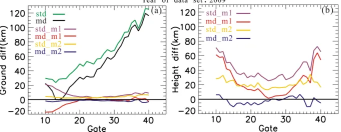
Fig. 8. (a) The standard and mean deviation of ground range between the results of model and the ray tracing for the data set in 2009. The green and black lines indicate the results of the standard SuperDARN model (std, md), the purple and red lines are for the linear fitting model (std m1, md m1), and the yellow and blue lines are for the quadratic fitting model (std m2, md m2). (b) The height deviation between the results of the fitting model and the ray tracing. The purple and red lines are for the linear fitting model (std m1, md m1), and the yellow and blue lines are for the quadratic fitting model (std m2, md m2).

new empirical virtual height model for SuperDARN HF radar backscatter by studying elevation angle data statisti-cally, using 5 years of backscatter from the Saskatoon Su-perDARN radar. The virtual height model was based on a low-order polynomial (quadratic) determined from the peak virtual height variations measured on the four Saskatoon beams. In their model, the range was divided into three seg-ments, 180 km to 790 km, 790 km to 2130 km, and greater than 2130 km, which corresponds to 1₂-hop E-region, 1₂-hop F-region and 11₂-hop F-region, respectively. The coefficients of the fitted virtual height polynomial were different for the three segments and the results showed that the ground range difference between the results from the new model and Eq. (4) can be reduced compared with the standard Super-DARN virtual height model, while large ground range un-certainties still existed due to the possibility of the misiden-tification of the radio wave propagation mode.

In this paper, using the combination of elevation angle data and ray tracing simulation, we have shown that the most

[image:8.595.129.470.267.399.2]

(9)

29 / 30

581

Figure 8

582

[image:9.595.311.547.59.254.2]

583

Figure 9

584

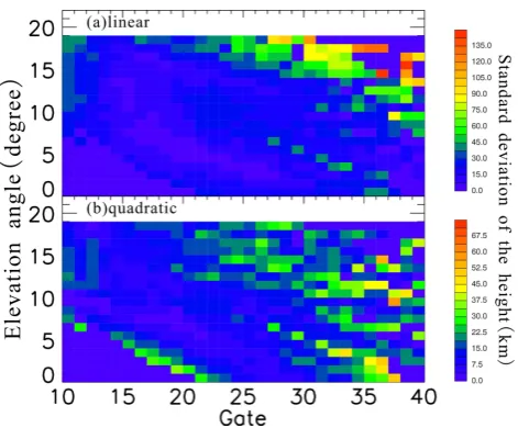
Fig. 9. Ground standard deviation of (a) the standard model of Su-perDARN, (b) the linear model and (c) the quadratic polynomial model determined by gate and elevation angle. The data set of 2009 is selected.

the new fitting model, the largest deviation greatly decreases to the level of 30 km. The standard deviation at large gates and low elevation angles, as well as the standard deviation at large elevation angles and small gates still exist, although the level of the deviation is not significant. The higher values of standard deviation located in these two regions are less ob-vious for the quadratic polynomial fitting model, as the co-efficient of quadratic term plays a growingly prominent role with the increasing gate and elevation angle in the deviation calculation. We also select the data set of 2008 to test the self-consistency of the new model in the same way (not shown) and the results show that the distribution of ground deviation in 2008 displays the same feature as that in 2009. The stan-dard deviation of echo height between the new fitting height model and the ray tracing for 2008 and 2009 are also esti-mated, with the distributions of deviation in range gate and elevation angles being similar in both years. The results of 2009 are shown in Fig. 10. The maximum deviation is in the region with large gate and high elevation angle, which can be at the level of 150 km for some range gates of the linear fit-ting model. This large deviation is significantly eliminated in the quadratic fitting model, although a very small amount of deviation (as large as 70 km) still exists in some large gates; most deviation can be reduced to be less than 40 km. Accord-ing to the analysis above, we conclude that the linear model is accurate enough for the determination of the location of the ionospheric irregularities.

We note here that the elevation angles determined by the SuperDARN interferometric technique can at times be diffi-cult to make due either to low signal to noise or poor coher-ence of the signals received by both antenna arrays. Further-more, some SuperDARN radars do not have an

interferom-Fig. 10. Height standard deviation of (a) the linear model and (b) quadratic polynomial model determined by gate and elevation angle. The data set of 2009 is selected.

eter array. Thus, while the technique described above does provide an improvement for some radars, it cannot be used over the whole array currently, nor at all times. Neverthe-less, we believe that for certain studies involving comparison between radars and other data sets, e.g. optical observations or low Earth orbiting spacecraft, the technique could, and should, be used to improve the range determination of the SuperDARN data.

It is also clear from the above discussion that there are a number of factors that could be taken into account when de-veloping models of location to be used in SuperDARN soft-ware, i.e. diurnal, seasonal and solar activity factors, signal frequency variations of the HF radar, and general spatial and temporal ionospheric electron density variability, which con-tribute to the random uncertainties and systematic deviation in the ray tracing. The electron density in the ionosphere, through which the SuperDARN HF rays propagate, is signif-icantly dependent on solar cycle and season. Generally, the critical frequency of the ionosphere is lower at solar mini-mum compared to solar maximini-mum and solar minimini-mum con-ditions might also be expected to increase the likelihood of the HF rays penetrating the ionosphere.

Besides the primary factors we consider, other possible factors are also worth considering if our approach is to be taken forward and the model presented here is to be improved further. However, taking into account of all these factors when developing new location models would lead to many additional complications. A more accurate model with as few factors involved as possible remains crucial to determine the location of ionospheric echoes for SuperDARN.

(10)

4 Summary

In this study, an attempt is made to statistically estimate the expected locations of ionospheric echoes that SuperDARN radar can observe by considering HF ray paths to the scat-tering area and by matching the predicted ranges and ele-vation angles of the echoes to the observed data. From the ray tracing simulation, the results showed two regions where SuperDARN radars can observe ionospheric irregularities through 1₂-hop propagation mode, one is at ranges of 300 km to 1200 km and heights of 70 km to 160 km, while the other is at ranges of 900 km to 1900 km and heights of 160 km to 300 km. Statistically, the most likely height of F-region echoes is∼240 km, although echoes’ height varies in indi-vidual cases. By calculating the ground range difference be-tween the results from the standard SuperDARN model and ray tracing using the data sets of Hankasalmi SuperDARN radar, we have proposed a new fitting location model and shown that the development of the adjusted location model, which is determined by both the measured slant range and elevation angle data, significantly improves the accuracy of estimations of ray propagation paths and scattering locations. This new fitting model can limit the ground range deviation to be less than 10 km and most of the height deviation to be less than 40 km, leaving predominantly the systematic devia-tion. The new model can provide an excellent representation of the location variation of ionospheric irregularities that the radar can observe.

Acknowledgements. This work was supported by the National

Nat-ural Science Foundation of China (NSFC grants 41031064), the National High Technology Research and Development Program of China (863 Program 2008AA121703), the Ocean Public Welfare Scientific Research Project, and the State Oceanic Administration of the People’s Republic of China (No. 201005017). We thank the University of Leicester radar group, which continuously operated the Hankasalmi HF radar and provided data used in this study. We also thank the Sodankyl¨a Geophysical Observatory for pro-viding the data. ML acknowledges support from STFC on grant ST/H002480/1.

Topical Editor K. Kauristie thanks A. V. Koustov and N. Nishi-tani for their help in evaluating this paper.

References

Andre, R., Hanuise, C., Villain, J. P., and Cerisier, J. C.: HF radars: Multifrequency study of refraction effects and localization of scattering, Radio Sci, 32, 153–168, 1997.

Barthes, L., Andre, R., Cerisier, J. C., and Villain, J. P.: Separation of multiple echoes using a high-resolution spectral analysis for SuperDARN HF radars, Radio Sci., 33, 1005–1017, 1998. Bates, H. F. and Albee, P. R.: Aspect sensitivity of F-layer HF

backscatter echoes, J. Geophys. Res, 75, 165–170, 1970. Bilitza, D. and Reinisch, B. W.: International reference ionosphere

2007: Improvements and new parameters, Adv. Space Res., 42, 599–609, 2008.

Chisham, G. and Pinnock, M.: Assessing the contamination of Su-perDARN global convection maps by non-F-region backscat-ter, Ann. Geophys., 20, 13–28, doi:10.5194/angeo-20-13-2002, 2002.

Chisham, G., Lester, M., Milan, S. E., Freeman, M. P., Bristow, W. A., Grocott, A., McWilliams, K. A., Ruohoniemi, J. M., Yeo-man, T. K., and Dyson, P. L.: A decade of the Super Dual Auro-ral Radar Network (SuperDARN): scientific achievements, new techniques and future directions, Surv. Geophys., 28, 33–109, 2007.

Chisham, G., Yeoman, T. K., and Sofko, G. J.: Mapping ionospheric backscatter measured by the SuperDARN HF radars – Part 1: A new empirical virtual height model, Ann. Geophys., 26, 823– 841, doi:10.5194/angeo-26-823-2008, 2008.

Danskin, D. W., Koustov, A. V., Ogawa, T., Nishitani, N., Nozawa, S., Milan, S. E., Lester, M., and Andre, D.: On the factors con-trolling occurrence of F-region coherent echoes, Ann. Geophys., 20, 1385–1397, doi:10.5194/angeo-20-1385-2002, 2002. Fejer, B. G. and Kelley, M. C.: Ionospheric irregularities, Rev.

Geo-phys., 18, 401–454, 1980.

Greenwald, R. A., Baker, K. B., Dudeney, J. R., Pinnock, M., Jones, T. B., Thomas, E. C., Villain, J. P., Cerisier, J. C., Senior, C., and Hanuise, C.: DARN/SuperDARN, Space Sci. Rev., 71, 761–796, 1995.

Jones, R. M. and Stephenson, J. J.: A versatile three-dimensional ray tracing computer program for radio waves in the ionosphere, US Dept. of Commerce, Office of Telecommunications, US Dep. of Comm., Washington, D.C., 1975.

Jones, T. B., Lester, M., Milan, S. E., Robinson, T. R., Wright, D. M., and Dillon, R. S.: Radio wave propagation aspects of the CUTLASS radar, J. Atmos. Sol.-Terr. Phy., 63, 99–105, 2001. Koustov, A. V., Andr´e, D., Turunen, E., Raito, T., and Milan, S. E.:

Heights of SuperDARN F region echoes estimated from the anal-ysis of HF radio wave propagation, Ann. Geophys., 25, 1987– 1994, doi:10.5194/angeo-25-1987-2007, 2007.

Macmillan, S. and Maus, S.: International Geomagnetic Reference Field- The tenth generation, Earth, Planets, and Space, 57, 1135– 1140, 2005.

Milan, S. E. and Lester, M.: A classification of spectral populations observed in HF radar backscatter from the E region auroral elec-trojets, Ann. Geophys., 19, 189–204, doi:10.5194/angeo-19-189-2001, 2001.

Milan, S. E., Jones, T. B., Robinson, T. R., Thomas, E. C., and Yeoman, T. K.: Interferometric evidence for the observation of ground backscatter originating behind the CUTLASS coherent HF radars, Ann. Geophys., 15, 29–39, doi:10.1007/s00585-997-0029-y, 1997a.

Milan, S. E., Yeoman, T. K., Lester, M., Thomas, E. C., and Jones, T. B.: Initial backscatter occurrence statistics from the CUTLASS HF radars, Ann. Geophys., 15, 703–718, doi:10.1007/s00585-997-0703-0, 1997b.

Milan, S. E., Davies, J. A., and Lester, M.: Coherent HF radar backscatter characteristics associated with auroral forms identi-fied by incoherent radar techniques: a comparison of CUTLASS and EISCAT observations, J. Geophys. Res, 104, 22591–22604, 1999.

(11)

auroral forms, Ann. Geophys., 19, 205–217, doi:10.5194/angeo-19-205-2001, 2001.

Press, W. H., Flannery, B. P., Teukolsky, S. A., and Vetterling, W. T.: Numerical recipes, Cambridge university press Cambridge, 2007.

Uspensky, M. V., Kustov, A. V., Sofko, G. J., Koehler, J. A., Vil-lain, J. P., Hanuise, C., Ruohoniemi, J. M., and Williams, P. J. S.: Ionospheric refraction effects in slant range profiles of auroral HF coherent echoes, Radio Sci., 29, 503–517, 1994.

Villain, J. P., Greenwald, R. A., and Vickrey, J. F.: HF ray tracing at high latitudes using measured meridional electron density distri-butions, Radio Sci., 19, 359–374, 1984.

Yeoman, T. K., Wright, D. M., Stocker, A. J., and Jones, T. B.: An evaluation of range accuracy in the Super Dual Auroral Radar Network over-the-horizon HF radar systems, Radio Sci., 36, 801–814, 2001.

Yeoman, T. K., Chisham, G., Baddeley, L. J., Dhillon, R. S., Karhunen, T. J. T., Robinson, T. R., Senior, A., and Wright, D. M.: Mapping ionospheric backscatter measured by the Su-perDARN HF radars – Part 2: Assessing SuSu-perDARN virtual height models, Ann. Geophys., 26, 843–852, doi:10.5194/angeo-26-843-2008, 2008.