Economics and Research Department
NBH WORKING PAPER
1998/2
Attila Csajbók:
Z
ERO-
COUPONY
IELDC
URVEE
STIMATION FROM AC
ENTRALB
ANKP
ERSPECTIVEOnline ISSN: 1585 5600
ISSN 1419 5178 ISBN 963 9057 19 3
Attila Csajbók: Economist, Economics and Research Department. E-mail: [email protected]
The purpose of publishing the Working Paper series is to stimulate comments and suggestions to the work prepared within the National Bank of Hungary.
The views expressed are those of the authors and do not necesserily reflect the official view of the Bank
Contents
1. THE YIELD CURVE AND MONETARY POLICY ... 7
1.1 WHAT IS A YIELD CURVE? ... 7
1.2 ZERO-COUPON AND YTM YIELD CURVES... 7
1.3 THE IMPORTANCE OF THE YIELD CURVE FOR MONETARY POLICY... 8
1.4 CONDITIONS UNDER WHICH THE YIELD CURVE CAN BE USED AS AN INDICATOR... 10
2. ZERO-COUPON YIELD CURVE ESTIMATION: ALTERNATIVE METHODS AND EXPERIENCE WITH HUNGARIAN DATA... 14
2.1 ESTIMATING THE ZERO CURVE WITH POLYNOMIALS AND SPLINES... 14
2.2 PARSIMONIOUS MODELS OF THE YIELD CURVE... 18
2.3 DATA ISSUES... 20
2.4 ZERO-COUPON YIELD CURVE ESTIMATIONS USING HUNGARIAN DATA... 22
2.5 THE PROPOSED ESTIMATION METHOD... 25
Abstract
Since in recent years a relatively liquid and transparent market of government securities has emerged in Hungary, it seems straightforward for the monetary authority to try to extract information about market expectations of future nominal interest rates and inflation from the prices of these assets. However, drawing a conclusion from the prices of T-bills and -bonds concerning either nominal interest rate- or inflation expectations is by far not an easy task, both because of its technical complexity and the assumptions which often remain implicit in the process. The primary motivation of this paper is to present some methods by which the major technical obstacle, i.e. the estimation of the zero-coupon yield curve from coupon-bearing bond price data can be done, and also to evaluate these methods in terms of suitability to current Hungarian data and practical use in monetary policy. In addition to this, I would like to emphasize and make explicit some often overlooked assumptions (especially the expectations hypothesis) needed to draw conclusions about market expectations of future nominal rates and inflation. Using the estimated zero-coupon rates, I also try to quantify the average difference between yields-to-maturities (YTMs) of coupon bonds and the corresponding zero-coupon rates in Hungary.
The structure of the paper is as follows:
Section 1.1 and 1.2 describe the basic concepts and definitions related to the yield curve, and compare zero-coupon curves with yield-to-maturity curves, focusing on the theoretical shortcomings of the latter. Section 1.3 defines implied forward rates, and shows how to interpret them. Section 1.4 focuses on the conditions which are necessary to hold if one wants to infere nominal interest rate and inflation expectations from the zero-coupon yield curve.
Part 2 deals with some methodological issues of the estimation of zero-coupon yield curves and compares alternative estimation methods on the basis of their applicability to Hungarian data and monetary policy purposes. Sections 2.1 and 2.2 give the descriptions of the two methods examined in detail in this paper, i.e. polynomial fit and “parsimonious” models. Section 2.3 deals with data issues that arise when we try to estimate yield curves using Hungarian bond price data. Section 2.4 lists some of the criteria which can be used to select a particular estimation method and (where it is possible) compares the methods applied to Hungarian data on the basis of these criteria. Section 2.5 contains the method proposed for future use in the NBH.
1.
The yield curve and monetary policy
1.1 What is a yield curve?
The yield curve can be defined most generally as a function which for any maturities (in a given range) gives the yields the market attaches to those maturities. In order to construct a yield curve, market yields/prices of certain securities (typically bonds and bills) with different maturities are usually used, although yield curves may be constructed from certain interest rate derivative (e.g. swaps) prices as well . These securities have to fall in the same risk category (at least in terms of default risk). In other words, there is a separate yield curve for each level of default risk. In practice yield curves are usually constructed using price/yield data of a special risk category, namely government securities, since this category has the biggest number of instruments in a wide maturity range, traded on a fairly liquid market.
1.2 Zero-coupon and YTM yield curves
If the zero-coupon yield curve (zero curve) is known, then the market price of a bond maturing m years ahead in the future and paying coupon C annually is given by the present value of its cash-flow, where the discount factors are calculated from the corresponding zero-coupon yields:
(
)
(
)
P C
i
C i
C R
i m m
=
+ + + + +
+ +
1 ( )1 1 2 2 1
( ) ... ( ) (1.1)
In (1.1) R is the redemption payment (principal), P is the price of the bond and the function i(t) , t = 1, ..., m is the zero curve itself. In order to be able to price coupon bonds, market participants always have to form some view about the zero curve. Since we cannot observe directly the discount rates market participants attach to different maturities, the zero curve will always have to be estimated, using price data for a set of coupon bonds1. From the price equation of an individual bond, only the yield-to-maturity (YTM) can be calculated. By definition, if the cash-flow of the bond is discounted using the YTM as the discount rate, the resulting present value is the market price of the bond:
(
)
(
)
P C
y m
C y m
C R y m m
=
+ + + + +
+ +
1 ( ) 1 ( ) 2 ... 1 ( ) , (1.2)
1 Unless there is a set of zero-coupon bonds which cover a sufficiently wide maturity spectrum.
where y(m) is the yield to maturity of a bond maturing in m periods.
Comparing (1.1) with (1.2) it is obvious that the yield-to-maturity is in some sense an “average” interest rate associated with the maturity of the bond (The YTM is identical to the concept of internal rate of return (IRR)).
By plotting the YTMs of bonds with different maturities against maturity, one can construct a “yield curve”, called the YTM-curve. It has to be stressed that theYTM-curve does not reflect the discount rates market participants attach to different horizons, so in this respect it cannot be called a yield curve. In practice however, it is often used as a crude approximation of the zero curve, since it is technically much less problematic to construct than the latter.
One of the theoretical shortcomings of the YTM-curve is related to reinvestment risk. When calculating the YTM, we implicitly assumed that coupon payments can always be reinvested at the YTM. In practice however, this is not necessarily true. The YTM usually differs from the ex post return on the bond (taking account of all coupon payments reinvested at the actual going rates), unless the interest rate does not change during maturity. This has an interesting implication for the YTM-curve: it is only consistent (with the implicit assumption we made when calculating the YTMs) if it is horizontal.
Another serious weakness of the YTM-curve stems from the so-called coupon effect, which is the fact that a bond with a higher coupon will have a higher yield-to-maturity than a bond with the same yield-to-maturity but a lower coupon. Because of the coupon effect, one should construct separateYTM-curves for each coupon size. But since in practice usually there are many different coupon sizes, there would be too few observations to construct the coupon-specific YTM-curves.
Even if such curves could be constructed, it would not be straightforward which one to use for further purposes, e.g. for pricing an instrument with a coupon for which no corresponding YTM curve is available.
None of these problems emerge in the case of a zero-coupon curve. Its main disadvantage is that its estimation is much more complicated, and usually depends on the assumed functional form of the discount function. Different assumptions about the discount function’s form may lead to different estimated zero curves, so the results are usually not unique in this sense. Nonetheless, both in the academic literature and in the fixed income business, the zero curve seems to be much more widespread.
1.3 The importance of the yield curve for monetary policy
forward-looking, as opposed to the goods- and labour markets, where past movements probably have a bigger influence on current prices. Because of these characteristics, asset prices are straightforward candidates for an indicator for central banks, as market expectations and their responses to monetary policy measures are captured in these prices the most quickly and most reliably2.
Among possible indicators for monetary policy, one that may reflect inflation expectations of agents would be of crucial importance, for at least two reasons. First, market expectations of inflation can be used as an input in the central bank’s model of inflation. Secondly, in a regime which explicitly or implicitly targets inflation, the difference between expected inflation and the inflation target is an important measure of credibility.
The reason why the yield curve is potentially very important for monetary policy is that, if some assumptions are satisfied (see below), one can derive market expectations of future nominal interest rate movements from the yield curve. If some other assumptions are satisfied, then the term structure of expected inflation can be recovered from the yield curve. If both sets of assumptions are satisfied, then not only the term structure of inflation but its future path as well can be derived from the zero curve.
One important concept related to the zero curve is the concept of implied forward rates. If the yield curve contains interest rates for maturities t1 and t2 (t2>t1), it also implies a forward rate for the period betweent1 and t2 in the following way:
(
(1 ( , )0 2)
2 0(
(1 ( , )0 1) (
1 0 1 ( , )1 2)
2 1+i t t t -t = +i t t t t- + f t t t -t ,
where:
i(t0, ti) : the spot rate for the period (t0, ti)
f(ti, tj) :. the implied forward rate for the period (ti, tj),
from which the implied forward rate can be calculated as:
(
)
(
)
f t t i t t i t t
t t t t t t ( , ) ( ( , ) ( ( , ) 1 2 0 2 0 1 1 1 1 1 2 0 1 0 2 1 = + + é ë ê ê ù û ú ú
2 Although asset markets are probably the closest to efficiency among all markets, at least two
If we fix the length of the implied forwards we want to examine, then we can calculate the implied forward curve for that particular maturity. Chart 1.1 shows a curve of 1-year implied forwards for Hungary on a particular day. The curve may be crudely interpreted3 as follows: market participants in Hungary on September 12, 1997 expected a slow decline of the1-year rate until the end of 1998 and then a more rapid (approx. 300 basis points p.a.) decrease in 1999 and 2000.
Chart 1.1
1-year implied forward curve 7-th degree polynomial fit
1997.09.12
10% 11% 12% 13% 14% 15% 16% 17% 18% 19% 20%
1997.09.12 1998.03.31 1998.10.17 1999.05.05 1999.11.21 2000.06.08 2000.12.25
The implied forward curve is particularly interesting for the monetary authority, since if the length of the implied forwards chosen is equivalent to the maturity of the central bank’s interest rate instrument, then the implied forward curve reflects market expectations of the future course of interest rate policy.
Another useful feature of implied forwards is that by subtracting the implied forward curve of a country from the corresponding curve of another country, and assuming that uncovered interest rate parity holds, one can get the expected future course of exchange rate depreciation. This can be particularly useful in countries with fixed exchange rate regimes, where it might be used in predicting speculative attacks.
1.4 Conditions under which the yield curve can be used as an indicator
So far I have mentioned some assumptions which have to be made so that the yield curve can be used as a meaningful indicator. Now I try to make them explicit.
3 As it was mentioned earlier, this interepretation is valid only if an important condition, namely the
The first such condition is the so-called expectations hypothesis (EH). If it holds in its pure form, then implied forwards are equivalent to expected future interest rates with the same maturity, so the implied forward curve reflects the expected future path of nominal interest rates. Formally, the expectations hypothesis can be written as:
(
1 0)
(
1 0 1)
(
1 1 2)(
1 2 3)
(
1 1)
0
0 0 0
+i t tn - = +i t t +E i t t +E i t t + E i t - t
t t
t t t n n
n
( , ) ( , ) ( , ) ( , ) ... ( , )
(1.3)
where:
i(t0 ,tn) : spot long (n-period) interest rate
i(t0 , t1): spot short (1-period) interest rate
Et0i(ti , ti+1): (i>0) the short expected today (at t0) for the i-th period
Or with continuously compounded interest rates4, and after some re-arrangement:
(
)
i t t
t t i t t E i t t E i t t E i t t
n n
t t t n n
( , )0 ( , ) ( , ) ( , ) .... ( , )
0
0 1 1 2 2 3 1
1
0 0 0
=
- + + + + - (1.4)
From the latter, it can be seen that if the EH holds, the long rate can be thought of as an average of the current and future expected short rates.
Contrary to the pure form of the EH, which requires (1.4) to hold as as exact equation, a somewhat less strict formulation allows for some difference between the two sides of (1.4) i.e. for a constant term premium. Whether the EH holds or not is of course an empirical question, which can be tested by econometric methods. However, with these methods only the joint hypothesis of rational expectations and the EH can be tested. If the joint hypothesis is not rejected, implied forwards not only do reflect market expectations of future interest rates, but they are also best predictors of future spot rates, since expectations are rational. In this case it is usually said that there is information in the term structure. If however, the joint hypothesis is rejected, i.e. the estimated term premium turns out to be large and time-varying, then the informational content of the term structure is poor.
The second important condition is the Fisher-equation, which is required to hold for one to be able to say something about expected inflation on the basis of nominal interest rates. According to the Fisher-equation, the nominal interest rate is the multiple of the real rate and expected inflation for the same maturity:
(
)
(
)
1+i t t( , )0 n = +1 r t t( , )0 n 1+Et0p( , )t t0 n (1.5)
where:
i(t0, tn) : spot nominal interest rate for the period (t0, tn)
r(t0, tn) : (ex ante) real interest rate for the period (t0, tn)
Et0p(t0, tn) : expected inflation at t0 for the period (t0, tn)
With continuous compounding:
i t t( , )0 n =r t t( , )0 n + Et0p( , )t t0 n (1.6)
In terms of the motivation of the monetary authorities (i.e. extracting information about inflation expectations from nominal interest rates) there are at least two problems with (1.6).
The first problem is that the ex ante real interest rate is not directly observable. This means that even if the Fisher-equation holds, in order to recover a term structure of inflation expectations we need a whole term structure of the real interest rate. A reliable fundamentals-based model which would yield such a real term structure is rarely available. In practice usually it can be assumed that at least at longer horizons, the ex ante real yield curve has a horizontal profile5. Some more brave assumptions equate ex ante real interest rates with currently observed ex post real interest rates. If one does not want to make such assumptions about the level of ex ante real rates, something still can be said about changes in inflation expectations. If no significant change has occurred in the fundamentals driving the ex ante real interest rate, one can attribute a change in the nominal interest rate to a change in expected inflation without saying anything about the levels.
The second problem of the formulation (1.6) of the Fisher equation is that it does not address the issue of uncertainty. Extending Fisher’s theory, Lucas (1978) showed that if intertemporally optimising agents face uncertain future income, prices and real interest rates, then the nominal interest rate in addition to the ex ante real rate and expected inflation will include a risk premium term as well. This risk premium may be negative as well as positive. The intuition behind this theoretical result is the following: if the expected covariance of future inflation and consumption growth is positive, then the risk premium is negative, since a decrease in consumption growth in this case coincides with an decrease in inflation, which generates a capital gain on fixed-rate nominal bonds, thus compensating agents for lower consumption. The capital gain is therefore a kind of (partial) insurance against a possible decrease in
5 However in transitional economies, where the capital/labour ratio is much less than in developed
consumption growth, and the negative risk premium (lower nominal rate) is the “fee” agents are willing to pay for this insurance. If, on the other hand, the expected covariance of future consumption growth and inflation is negative, the capital loss on fixed bonds will only make the situation worse when the rate of growth of consumption decreases, so in this case agents require a positive risk premium on fixed bonds and nominal interest rates will be higher than the sum of ex ante real rates and expected inflation.
If nominal rates are determined by these three components (ex ante real rates, expected inflation and the risk premium), it is straightforward to ask whether monetary policy makes a mistake (and if it does, to what extent) when it simply attributes changes in nominal rates to changes in expected inflation. There is anecdotal evidence that for example Fed policymakers in the 1980s and ‘90s attributed changes in long rates to changes in inflation expectations. The necessary condition for such a conclusion to make any sense is that long-term ex ante real rates are stable and that risk premia are stable and small in magnitude. Examining U.S. quarterly data (a time series of 35(!) years up to 1994) Ireland (1996) found the ex ante real rate in the examined period surprisingly stable and the risk premium component in the price of nominal bonds small, which means that Fed policymakers did not make a mistake when attributing changes in long nominal rates to changes in long-term inflation expectations.
2.
Zero-coupon yield curve estimation: alternative methods and
experience with Hungarian data
2.1 Estimating the zero curve with polynomials and splines
Both in the case of simple polynomial- and spline-based estimation of the zero curve, we assume that the discount function d
( )
t , which gives the discount factors attached by the market to different horizons t, can be written as a sum of k basis functions (plus 1):d( )t a f tj j( ) j
k
= + å =
1
1
, (2.1)
where:
fj(t) : the j-th basis function
aj: the coefficient of the j-th basis function
Once we know the discount function d
( )
t , the zero-coupon yield curve can beuniquely derived from the following definition:
( )
( )
(
)
d t
i t t
= +
1 1
So the zero curve is given by:
( ) ( )
i t =d t -1/t -1 (2.2)
Available data for estimating the zero curve for a given day:
The net market price and accrued interest (piand ai, i=1,...,n) of n bonds and T-bills, and their cash-flows cij (j=1,...,mi), where mi is the number of remaining cash-flow elements (i.e. coupon payments and redemption) of the i-th Treasury security, as well as the function t(cij) which gives (in years) the distance in time from today of the various cash-flow elements.
Using matrix notation, these input data can be organised in a more compact way. Let
contain the pi and aii elements (i=1,..., n) and let d'
( )
m be a 1 x q vector, the i-th element of which is the discount factor corresponding to the maturity mi. Using this notation, the gross price vector of the n instruments is given by:( )
p ai'+ =' d' m C (2.3)
I will return to the matrix notation later, but in order to derive the regressions which yield the estimates of the coefficients aj in (2.1) we need the non-matrix notation: The market price of the i-th instrument using non-matrix notation:
( )
(
)
pi aii t cil cil
l mi
+ = å
=1d
(2.4)
Substituting (2.4) into (2.1):
( )
(
)
(
( )
)
pi aii a f t cj j il c c a f t c c
j k
il l
m
il j j il
j k il l m l m
i i i
+ = é + å ëê
ù ûú =
å å + åå
=
=1 1 1 =1 =1 =1 (2.5)
Rearranging (2.5):
( )
(
)
pi aii cil aj f t c c
j k
j il il
l m
l
mi i
+ -å = å å
= =
=1 1 1 (2.6)
Introducing the following notation
yi pi aii cil
l mi
= + - å
=1
( )
(
)
xij f t cj il cil
l mi
= å
=1 ,
(2.6) can be written as:
yi a xj
j k
ij
= å
=1 .
(
)
$ ' '
a= X X -1X y
, where
$
a is the k x 1 vector of estimated coefficients
X is the n x k matrix of consisting of the elements xij
y is the n x 1 vector of the elements yi
Substituting the estimated parameters a$ into (2.1) we get the estimated discount function, from which the estimated zero curve can be derived using (2.2).
As it is clear from the above procedure, the assumption about the form of the basis functions fj(t) is crucial in the estimation. In the case of fitting a simple polynomial, in (2.1) k = n, and the basis functions take the simple form fj(t)= tj, i.e. d
( )
t is a (k=)n-th order polynomial in t. In the case of polynomial spline fitting the definition of the basis functions is more complicated and it depends on the location of the given cash -flow element in time relative to the so-called knot-points. McCulloch (1975) presents a possible cubic spline basis.
The criticism that most frequently emerges in connection with simple polynomial fitting is centered around the trade-off between goodness-of-fit and stability. The higher the degree of the applied polynomial, the less “smooth” is the resulting yield curve and the less stable are the estimated parameters. If the order of the polynomial is too low on the other hand, the goodness-of-fit will not be satisfactory. Since the maturity of the majority of the instruments used for the estimation is typically short (less than 1 year), the goodness-of-fit is usually worse in the case of longer maturities. If we try to remedy this problem by increasing the order of the polynomial, then the curve will be more flexible in the longer horizon, but this may often lead to a strange result: the implied forward curve, instead of converging to some long-run level, may in fact become quite steep (or start oscillating) even at horizons which are long, but shorter than the maturity of the longest instrument. Economic intuition suggests that beyond some time horizon nominal interest rate expectations of agents should converge to a certain level, as they have less and less information to distinguish between expected interest rates with maturity m and say,
m + 1 as m increases. In the light of this intuition, implied forwards at the longer section of the yield curve, which change very much as maturity increases are implausible.
“smooth”6. The spline is this curve consisting of different polynomials, which yields satisfactory goodness-of-fit without the instability resulting from fitting high-degree polynomials.
Nevertheless, estimation of the zero curve with splines is not without problems either. The major problem is that the number and location of the knot points is chosen usually arbitrarily or at best according to some rules of thumb. The number of knot points determines the flexibility of the spline. Too few knot points result in bad fit while with too many knot points the estimated curve will adjust to outliers too readily, a trade-off similar to that observed in the case of fitting simple polynomials. Regarding the optimal number of knot points the literature mentions some rules of thumb: for this purpose, McCulloch (1975) for example proposes the nearest integer to the square root of the number instruments used for the estimation.
The two most common strategies for determining the location the knot points are fixing the knot points at predetermined horizons (e.g. at 1, 5 and 10 years) or placing them in a way that an equal number of instruments mature between each consecutive knot points. The advantage of the latter is that changes in the maturity structure of public debt are reflected quickly and automatically in the placement of knot points. Its disadvantage is that daily changes in the knot point positions alone may result in changes in the estimated term structure even in cases when the “true” term structure has not changed.
Although it improves the trade-off between goodness-of-fit and stability, spline-based estimation may result in implausible behaviour of implied forwards at longer horizons. Moreover, so far we have only discussed implied forward behaviour inside the longest observable maturity, while in practice one of the important applications of the yield curve in emerging bond markets where the length of the maturity spectrum may still be short is extrapolation beyond the longest current maturity in order to price new, longer instruments (in the case of Hungary for example, with a term structure length of 5 years pricing the 10-year T-bond likely to be issued soon is a relevant problem.). However, polynomials and splines, since they only fit on existing maturities and are not asymptotically restricted (i.e. the estimated curves are explosive) are not appropriate for extrapolation purposes.
An a priori assumption about the discount function d
( )
t that it is positive and monoton decreasing. In practice however, the discount function estimated by a polynomial or a spline may take negative values or may have a positive slope. In these cases the estimated zero curve is not interpretable. This problem has indeed emerged for short periods in the sample when I tried to reconstruct the Hungarian zero curve using the polynomial and the spline method.
6 Technically, “smoothness” in this context means that the around each knot points of the n-th order
2.2 Parsimonious models of the yield curve
In recent years and especially among central banks the use of so-called parsimonious models (functional forms) of the yield curve have become increasingly popular. In the case of polynomial and spline regressions the emphasis is on the discount function: we assume that it can be constructed as a linear combination of a certain number of basis functions and after assuming some functional form for the basis functions we estimate the coefficients of those. The first proponents of parsimonious
models, Nelson and Siegel (1987) assumed a functional form directly for the
instantaneous forward curve. This functional form can be derived from their assumption that the path of instantaneous forwards is described by a second-order differential equation7:
( )
(
)
(
)
f m =b +b e-mt +b m t e-mt
0 1 / 2 / / (2.7)
where f(m) is the instantaneous forward rate for the period m periods ahead,
b b b t0, 1, 2, are parameters affecting the shape of the forward curve.
Integrating (2.7) from zero to m and dividing the result by m we get the
(continuously compounded8) spot interest rate for maturity m:
( )
(
)
(
)
(
)
i mc =b + b +b -e-mt m t -b e-mt
0 1 2 1 2
/ / / / (2.8)
From the spot rate the discount function can be easily derived as:
( )
( )d m =e-i m mc (2.9)
But what are the advantages of focusing directly on the forward curve instead of the discount function? As it was mentioned before, there are some a priori assumptions about the shape of the forward curve on the basis of which some estimated yield curves and the implied forward curves can be rejected as implausible results. For example, such a priori assumption is that forwards on longer horizons should converge to some asymptotic value, as agents have less and less information to discriminate between expected rates as the horizon of these rates get longer. But if we select estimation methods on the basis of whether this a priori assumption is satisfied or not, why don’t we use an estimation method which assures that it is
7 For practical reasons Nelson and Siegel made the further restriction that the two roots of this
differential equation are equal so it reduced to (2.7).
8 The continuously compounded equivalent i
c(m) of the discrete (annual) interest rate i(m) is given by:
( )
(
( )
)
always satisfied? Nelson and Siegel did just that when they assumed the functional form (2.8) for the yield curve, which is sufficiently flexible to provide the typical (increasing, inverted and hump-shaped) forms of the yield curve while satisfying most of the a priori assumptions. Moreover it is “parsimonious”, since it describes the shape of the yield curve using four parameters only. A further advantage of this specification is that the parameters can be interpreted. Since
( )
mlim®¥i mc =b0 .
b0 is the asymptotic (“very long”) rate towards which the spot rate (as well as the
forward rate) converges. It is also true that
( )
m®0i mc = 0 + 1
lim b b
which means that the sum of b0 and b1 gives the instantaneous spot rate. In much
of the empirical work, the instantaneous spot rate is thought of as an approximation of the overnight rate. Parameter t influences how “fast” (i.e. at what horizon) the spot rate converges to the asymptotic rate while b2 affects the size of a possible
“hump”. The functional form chosen by Nelson and Siegel satisfies the a priori requirements based on economic intuition about the shape of the forward curve, but this means that it usually fits the data worse than yield curves estimated by splines or polynomials. Therefore it is not surprising that this method become much more popular among central banks, which are interested in the basic shape of the yield curve than among profit-oriented market participants, who use yield curves to detect mispriced instruments.
In order to increase the flexibility of the Nelson-Siegel yield curve, Svensson (1994) added an extra term to (2.8):
( )
(
)
(
)
(
)
i m e m e e
m e
c
m m m m
= + + - - + æ -
-è
ç ö
ø ÷
- - -
-b b b t b b
t
t t t t
0 1 2 1 2 3
2
1 1 1 1
2
2
/ / / / / /
/ (2.10)
This extension basically allows for another “hump” in addition to that in the original Nelson-Siegel formulation.
discount factors d'
( )
m according to (2.3), we get an initial value of estimated prices. Using a numerical optimisation method (e.g. Gauss-Newton) minimising the sum of squared differences between the estimated and observed prices, we get the final estimate of the parameter vector.An alternative would be to minimise the sum of squared differences of observed yields and the estimated yields (IRRs) calculated at each iteration from the estimated prices. Since there is a non-linear relationship between coupon bond prices and yields, the result of this procedure is not equivalent to that of the price-error minimising procedure. The duration of instruments with short remaining maturities, and thus the elasticity of their prices with respect to yield changes is smaller than that of instruments with long maturities, therefore the price-error minimising method implicitly places less weight on shorter maturities relative to the yield-error minimising estimation. Thus, the former will fit relatively better at longer horizons while the latter at short horizons. The choice between price or yield-error minimising should therefore primarily depend upon the motivation of the estimation (e.g. whether monetary policy is more interested in shorter or longer-horizon interest rate expectations). In practice it also should be taken into account that minimising yield-errors requires much more computer time, since at each iteration, the IRRs of all instruments have to be calculated - again by an iterative procedure.
2.3 Data issues
The daily estimations of the Hungarian zero curve use the secondary market prices of T-bills and T-bonds (32-38 instruments) which are included in the obligatory electronic quoting system of primary dealers. Since it is highly unlikely that in any given moment there are transactions for all these instruments, “market prices” used in the estimation are not actual transaction prices, but the (arithmetic) averages of the best bid and ask prices quoted for all the instruments in a certain moment. More specifically, the price data is acquired by saving the Reuter’s HUBEST page at a randomly chosen moment within the trading hours. Of course, it is questionable whether a price constructed this way really represents the market price. This is supported by the obligation of the primary dealer quoting the best (bid or ask) price to accept any offer at this price up to a limit of HUF 50 million (USD 250 thousand, which is a reasonable amount for a single transaction in the Hungarian bond market).
Exchange are known to be unreliable, some transactions suggest that a part of market participants use this channel for hidden transfers.
Given all these problems related to transactions data, I decided to use the average of best bid and ask prices.
[image:19.612.130.499.287.519.2]The maturities of the instruments used for the estimation fall between 3 months and 5 years (Fig. 2.1). Approximately two-thirds of these instruments mature within a year. Due to the fact that the longest (5-year) Hungarian bonds were not issued very long ago, still there is a 7-month gap in the yield curve between approx. 3 and 3.5 years, which is the difference between the maturities of the most recently issued 3-year and the first issued 5-year T-bonds. This gap will of course get smaller as new 3-year bonds are issued.
Figure 2.1
Yields-to-maturities and the estimated (Svensson-) zero-coupon curve 1998. 05. 21
15% 16% 16% 17% 17% 18% 18% 19% 19% 20%
0 0.5 1 1.5 2 2.5 3 3.5 4 4.5 5
zero curve YTMs
The daily time series of T-bill and -bond prices start at the settlement date of October 11, 1996 and are available with a daily frequency since then.
2.4 Zero-coupon yield curve estimations using Hungarian data
In the next section some criteria are provided in order to support the NBH in the choice between different estimation methods.
1. Goodness-of-fit
The measure of goodness-of-fit for one particular day could be the sum of squared differences of estimated and observed prices divided by the number of instruments used for the estimation (Root Mean Squared Error, RMSE):
(
)
RMSE
p p
n
i i
i n
= å= - $ 2 1
Calculating the average and standard deviation of the RMSE for the whole sample for different methods, we can compare their pricing efficiency. On this field we expect the polynomial and spline methods to perform better.
2. Consistency of the yield curve and the implied forward curve with economic intuition
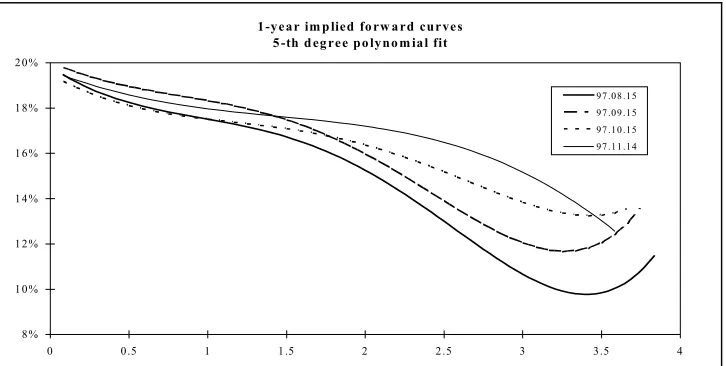
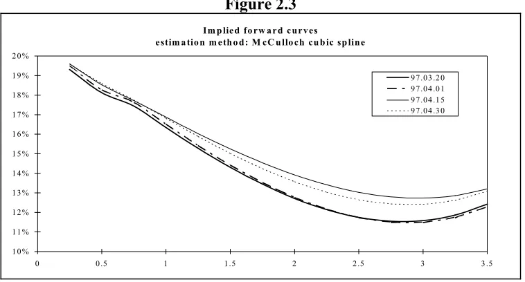
[image:20.612.133.496.517.700.2]Both the polynomial and the cubic spline method proved to be problematic in this respect. For quite a few days in the sample, the implied forward curve bent up at the 3-3.5 year horizon (Fig. 2.2-2.3), which is a rather implausible result as it was mentioned earlier.
Figure 2.2
1-year im p lied fo rw a rd curves 5 -th d eg ree po lyno m ial fit
8% 1 0% 1 2% 1 4% 1 6% 1 8% 2 0%
0 0.5 1 1 .5 2 2 .5 3 3.5 4
Figure 2.3
Im p lied fo rw a rd curves
estim a tio n m eth o d: M cC u llo ch cu b ic sp line
10% 11% 12% 13% 14% 15% 16% 17% 18% 19% 20%
0 0.5 1 1.5 2 2.5 3 3.5
97.03.20 97.04.01 97.04.15 97.04.30
Another problem with higher (5th and 7th) -degree polynomials and the spline is that there are certain periods for which the discount function becomes negative at certain maturities, therefore yield curves for these days cannot be calculated using these methods. Because of this problem, more than one month of observations are missing from the yield curve time series estimated by 5th and 7th order polynomials and some two weeks from that estimated by the McCulloch cubic spline. Since it is quite important that the NBH choose a method by which a complete time series can be reconstructed, this seems to be a significant disadvantage. This kind of problem (the negativity of the discount function) cannot emerge in the case of parsimonious models. On the other hand, the Nelson-Siegel and Svensson methods have other disadvantages, but these seem to be less serious. The fact that the parameters of the parsimonious models have some economic meaning was mentioned as an advantage. However, when I did unrestricted estimation of these models, the asymptotic forward rate often turned out to be negative. This was always offset by the short- and medium term components up to the longest existing maturity (5 years) and usually well beyond that, so that the yield curve and the implied forward curve did not take on implausible values in this segment. The result that the asymptotic forward rate takes on negative values is probably due to the short length of the yield curve and the fact that it is strongly inverted. Nevertheless, even if some of the parameters can no longer be interpreted, the estimated yield curve is still reliable up to the longest existing maturity.
As it was shown before, polynomial and spline estimation can be done by linear regression, so the estimated yield curve is always unique. Parsimonious models can only be estimated using numerical methods, therefore the result may be influenced by the initial parameter values chosen for the estimation. Iterations may lead to a local minimum or the objective function may not converge at all.
One strategy may be to choose the same vector of initial values for each day. Another reasonable strategy is to use the previous day`s estimates as the initial parameters for a given day.
The numerical method I used for the estimations is a quasi-Newton algorithm provided as an option in the Excel Solver software. A general result from a (not too comprehensive) sensitivity study of the applied method showed that whenever the initial values described a term structure which was plausible (no negative values) and resembled in its basic features to the probable Hungarian yield curve (i.e. was
downward-sloping ), the procedure converged and probably captured (was not
significantly different from) the ”true”underlying yield curve.
Based on this result I estimated the yield curve with the Svensson method using a single initial value vector for the whole sample. Fig. 2.4 contains the evolution of the yield curve along the sample, showing the so-called ”benchmark” maturities (i.e. the ones that correspond to the maturities of YTMs published daily by the SDMA, that is 0.25, 0.5, 1, 2, 3 and 5 years). The interpretation of yield curve movements is beyond the scope of this paper.
Figure 2.4
Zero-coupon rates at different maturities
13% 15% 17% 19% 21% 23% 25%
96.09.22 96.12.31 97.04.10 97.07.19 97.10.27 98.02.04 98.05.15
In addition to those estimated by the Svensson method, Fig. 2.5 contains the zero-coupon rates estimated by the McCulloch cubic spline9 (except the period when the estimated discount function was negative). Apart from the 3-month rate, there seem to be only small differences between estimated zero-coupon yields, although these differences become more significant when one looks at implied forwards.
Figure 2.5
Zero-coupon rates (at the maturities of Fig. 2.4) estimated with two alternative methods
13% 15% 17% 19% 21% 23% 25% 27%
96.09.22 96.11.11 96.12.31 97.02.19 97.04.10 97.05.30 97.07.19 97.09.07 97.10.27 97.12.16 McCulloch cubic spline Svensson
4. International comparability
Assuming that uncovered interest parity holds the comparison of zero curves of two countries yields estimates of expected depreciation of the home currency vis-à-vis the currency of the other country. In this respect it is important that the two curves be comparable, i.e. they should be estimated using the same method, if possible. The Svensson method seems to have an obvious advantage from this point of view. As it can be seen from the Appendix the majority of central banks in developed countries apply this method in the estimation of the zero-coupon curve.
2.5 The proposed estimation method
On the basis of the above criteria, I propose that the NBH uses the Svensson method for the daily estimation of the Hungarian zero-coupon curve. In my opinion, the most important criterion when choosing between alternative methods is that the resulting implied forward curves have a plausible shape, which is not guaranteed if polynomial or spline methods are used. The fact that the zero curve estimated by parsimonious
models is non-unique does not seem to cause a problem in practice. The Svensson functional form is able to capture a more complex term structure than the Nelson-Siegel functional form. The use of a model which allows for a more complex functional form seems to be justified for the description of the Hungarian term structure, although more testing is necessary in this direction. A further advantage of the Svensson method is its widespread use among central banks in developed countries.
3. Application: Bias in the Hungarian “benchmark” yield curve
Summary
YTM yield curves do not attach the discount rates used by the market to different maturities, but the complex averages of these. Therefore YTM yield curves usually are biased, in the sense that they systematically under- or overestimate market rates unless the underlying zero-coupon curve is close to horizontal. In the case of a positively-sloped zero curve, YTM yields will be lower, while with an inverted zero curve they will be higher than the corresponding zero-coupon yields.
Although the slope of the Hungarian zero-coupon curve changed significantly during 1997, it was always negative. Consequently, the “benchmark” yield curve of the State Debt Management Agency (SDMA), which consists of YTMs of 6 representative maturities, was biased upwards. The aim of the following Section is to quantify this bias. This was not possible before, since there were no estimations of zero-coupon yield curves which reflected the “true” discount rates the market attaches to different horizons.
According to the results, a very crude estimation of inflation expectations (assuming a constant real interest rate and term premium) for different horizons using the SDMA “benchmark” yields, overestimated 1 and 2 years ahead expected annual inflation by approx. 50 basispoints on average and 3 and 4 years ahead expected annual inflation by 160-180 basispoints on average.
*
The following part deals with the sources of inherent bias in YTM yield curves in detail, using the formulas in Section 1.
element in the i(t) increasing series, that is it will be lower than i(m). Obviously, for a negatively sloped zero-coupon curve, it is the opposite, i.e. y(m) > i(m). The bias is bigger the more steeply sloped the yield curve (in absolute value), the longer the maturity that we examine (the bigger m) or the bigger the coupon on the bond used to
calculate y(m). The picture is not so clear if the underlying zero curve is not
monotonic, but for monotonic zero curves (throughout 1997, the Hungarian zero curve was monotonic) the existence and the direction of the bias is not questionable. The second theoretical objection against the YTM yield curve is that for bonds with the same maturities the one with a bigger coupon will have a higher YTM (this is the so-called coupon effect). Therefore, the right procedure would be to construct a separate YTM yield curve for each coupon size. In practice this is problematic because there are a lot of different coupon sizes on the market, so the number of observations for single YTM curves would not be sufficiently large. If one constructed a single YTM curve using bonds with different coupons, the most obvious problem would be if there were two YTMs for the same maturity. In this case it would be hard to decide which YTM can be taken as the rate of return expected by the market for that maturity. The coupon problem emerges in the Hungarian data as well, since the coupon sizes of the outstanding marketable T-bond stock vary in quite a wide range (14-24%).
The SDMA “benchmark” yield curve - beside all the disadvantages of YTM yield curves in general - has some other “unpleasant” features. It contains YTMs for only 6 maturities (3 and 6 months, 1, 2, 3 and 5 years), and these always belong to only one instrument, i.e. the one that matures closest to the given maturity. Thus, the SDMA “benchmark” uses only a fraction of the information available on the market (currently there are 38 instruments in the primary dealers’ obligatory quoting system). Another source of bias is that what is referred to as say, the 5-year “benchmark” yield, may in fact be the YTM on a bond with 4.5 years remaining maturity. If the zero-coupon curve is negatively sloped, then this bias has a positive sign, since if we average the decreasing series of zero-coupon yields on a shorter maturity, we get a higher average, i.e. a higher YTM. Thus, the bias caused by shortening maturity has the same sign as the bias caused by a non-horizontal zero-coupon curve. In the following we attempt to quantify the total bias in YTMs and do not try to separate it between these two sources10.
10 However, it is worth to look at the maximum amount of bias caused by maturity shortening in the
A further problem stemming from the construction of the “benchmark” yield curve is that any time the basis of a “benchmark” yield of a given maturity is switched to another instrument (e.g. when the basis of the 5-year “benchmark” is switched from a bond with a 4.5-year remaining maturity to a newly issued 5-year bond) there may be jumps in the YTMs, of course these are expected to be significant only in the case of rarely issued, long maturities.
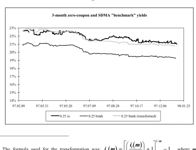
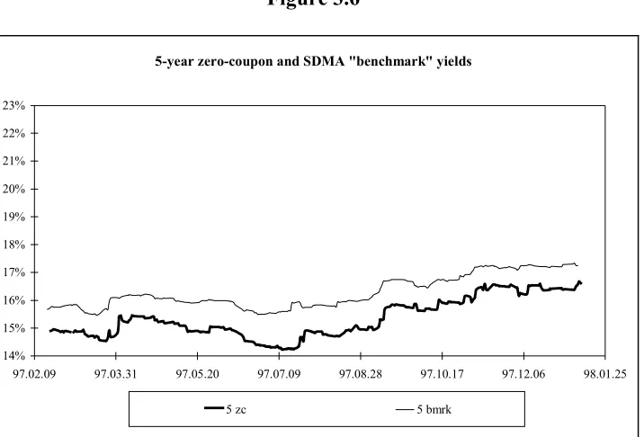
In order to quantify total bias I compared “benchmark” YTMs with zero-coupon yields of the corresponding maturities (i.e. 3 and 6 months, 1, 2, 3 and 5 years), estimated using the Svensson method. The sample period ranged from February 17, 1997 (the first publication of the SDMA “benchmark”) to January 8, 1998. Figures 3.1-3.6 contain the results (all charts have been drawn to the same scale in order to make the biases on different maturities comparable). The 3 and 6 month “benchmark” yields, according to the Hungarian convention, are linearly annualised (“simple”) yields while the 1-year and longer “benchmark” yields, as well as all the zero-coupon yields are compounded. Therefore I transformed the 3 and 6-month
benchmark yields into compounded ones11, and Figures 3.1. and 3.2 show
[image:26.612.115.506.376.675.2]“benchmark” yields according to both compounding conventions.
Figure 3.1
3-month zero-coupon and SDMA "benchmark" yields
14% 15% 16% 17% 18% 19% 20% 21% 22% 23%
97.02.09 97.03.31 97.05.20 97.07.09 97.08.28 97.10.17 97.12.06 98.01.25
0.25 zc 0.25 bmrk 0.25 bmrk (transformed)
11 The formula used for the transformation was: i m
( )
i m( )
m
k l
m = æ
è
ç öø÷ + é
ë
ê ù
û ú
-1 1 1
1
/
/
Figure 3.2
6-month zero-coupon and SDMA "benchmark" yields
14% 15% 16% 17% 18% 19% 20% 21% 22% 23%
97.02.09 97.03.31 97.05.20 97.07.09 97.08.28 97.10.17 97.12.06 98.01.25
0.5 bmrk 0.5 zc 0.5 bmrk (transformed)
Figure 3.3
1-year zero-coupon and SDMA "benchmark" yields
14% 15% 16% 17% 18% 19% 20% 21% 22% 23%
97.02.09 97.03.31 97.05.20 97.07.09 97.08.28 97.10.17 97.12.06 98.01.25
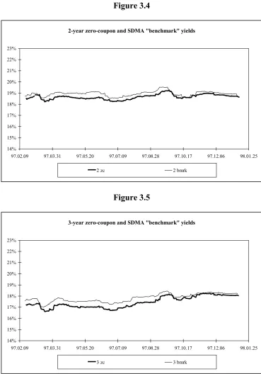
[image:27.612.125.503.180.648.2]Figure 3.4
2-year zero-coupon and SDMA "benchmark" yields
14% 15% 16% 17% 18% 19% 20% 21% 22% 23%
97.02.09 97.03.31 97.05.20 97.07.09 97.08.28 97.10.17 97.12.06 98.01.25
[image:28.612.128.501.141.380.2]2 zc 2 bmrk
Figure 3.5
3-year zero-coupon and SDMA "benchmark" yields
14% 15% 16% 17% 18% 19% 20% 21% 22% 23%
97.02.09 97.03.31 97.05.20 97.07.09 97.08.28 97.10.17 97.12.06 98.01.25
Figure 3.6
5-year zero-coupon and SDMA "benchmark" yields
14% 15% 16% 17% 18% 19% 20% 21% 22% 23%
97.02.09 97.03.31 97.05.20 97.07.09 97.08.28 97.10.17 97.12.06 98.01.25
5 zc 5 bmrk
[image:29.612.107.503.550.599.2]It can be seen from Figures 3.1-3.6 that while the difference between SDMA “benchmark” and zero-coupon yields is not significant at the 3 and 6-month and the 1-year maturities, there are significant biases in the case of 2, 3 and 5-year maturities. Table 3.1 gives the average differences along the whole sample for all the maturities examined. Average differences should be interpreted with a caution: when the underlying zero curve is more steeply sloped in absolute value (e.g. from the beginning of the sample period until mid-June, 1997) the bias is bigger than the average. After the yield curve started to become less inverted in July 1997, the bias in the SDMA “benchmark” decreased, as it is well illustrated in Fig. 3.5 for example.
Table 3.1
Average difference of zero-coupon and SDMA “benchmark” spot rates
maturity 0.25 0.5 1 2 3 5
avg. difference in bps -2 9 2 34 49 100
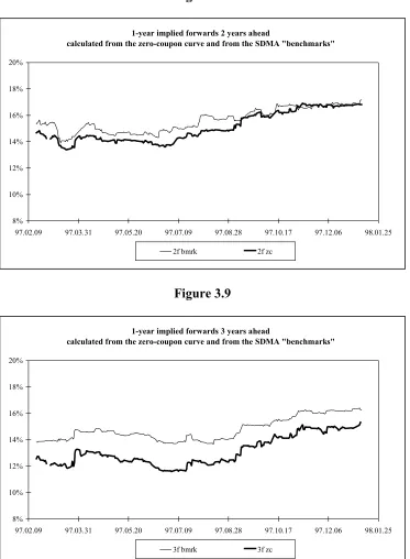
Figures 3.7-3.10 show 1-year implied forwards on 1, 2, 3 and 4-year horizons calculated from the SDMA “benchmark” and from the zero-coupon yield curve. Thus, for example Figure 3.9 shows the 1-year nominal interest rate expected 3 years form today12, calculated both ways. The differences between implied forwards are much bigger than those between spot rates. Of course, the whole amount of these differences appear in the expected inflation rates calculated with the crude method. Average differences for the whole sample are shown in Table 3.2. So if one used the above mentioned crude method, he/she overestimated 1 and 2-year-ahead expected annual inflation by approx. 50 basispoints and 3 and 4-year ahead expected inflation by 160-180 basispoints.
Table 3.2
Average difference of 1-year implied forwards calculated from the zero-coupon yield curve and the SDMA “benchmarks”
years ahead 1 2 3 4
[image:30.612.127.499.285.599.2]avg. difference in bps 58 53 166 180
Figure 3.7
1-year implied forwards 1 year ahead
calculated from the zero-coupon curve and from the SDMA "benchmarks"
8% 10% 12% 14% 16% 18% 20%
97.02.09 97.03.31 97.05.20 97.07.09 97.08.28 97.10.17 97.12.06 98.01.25 1f bmrk 1f zc
12 It should be stressed that implied forwards equal expected nominal rates only if the expectations
Figure 3.8
1-year implied forwards 2 years ahead
calculated from the zero-coupon curve and from the SDMA "benchmarks"
8% 10% 12% 14% 16% 18% 20%
[image:31.612.128.499.129.364.2]97.02.09 97.03.31 97.05.20 97.07.09 97.08.28 97.10.17 97.12.06 98.01.25 2f bmrk 2f zc
Figure 3.9
1-year implied forwards 3 years ahead
calculated from the zero-coupon curve and from the SDMA "benchmarks"
8% 10% 12% 14% 16% 18% 20%
Figure 3.10
1-year implied forwards 4 years ahead
calculated from the zero-coupon curve and from the SDMA "benchmarks"
8% 10% 12% 14% 16% 18% 20%
97.02.09 97.03.31 97.05.20 97.07.09 97.08.28 97.10.17 97.12.06 98.01.25 4f bmrk 4f zc
Figures 3.7-3.10 have another message as well. It is clear that implied forwards calculated from the zero-coupon curve are much more volatile than those calculated from the “benchmarks”, and the longer the maturity, the bigger the volatility. Suppose we want to use the above mentioned crude method to estimate inflation expectations with a daily frequency. Although the inherent bias is removed if we use the implied forwards calculated from the zero curve instead of those calculated from the “benchmark”, it would be appropriate to “smooth” the daily estimates of inflation expectations some way (e.g. using a moving average) because the higher volatility not necessarily stems from similarly volatile inflation expectations but more likely from
Appendix: Central bank zero-coupon estimation methods in
developed countries
Meeting on the estimation of zero-coupon yield curves Basle, 5th June 1996
Summary of estimation approaches
Central Bank Estimation method13 Belgium Cubic spline
Canada Enhanced third-order polynomial (8 coefficients) (experiments with NS & ExNS)
Finland ExNS(P)
France · NS(P) or
· ExNS(P) (restricted at short end)
Germany Fit of polynomial through observed redemption yields (experiments with NS & ExNS)
Italy · Cubic spline
· Cox, Ingersoll & Ross one and two factor model · Swap rate yield curves
Japan 5th order spline Netherlands
--Norway · Cubic spline · NS
Spain · NS(P)
· ExNS(P)
Sweden ExNS(Y) (restricted at short end) Switzerland ExNS(P)
United Kingdom ExNS(P) (adjustments for tax effects) United States · NS(Y) & ExNS(Y) (restricted at long end)
· Smoothing splines (penalty for excess roughness)
13 “NS=Nelson-Siegel,ExNS=extended Nelson-Siegel (=Svensson), estimation method minimises
References
Ireland, P. N. (1996) Long-term interest rates and inflation: a Fisherian approach,
Federal Reserve Bank of Richmond Economic Quarterly,Winter 1996, 21-35.
Lucas, R. E. (1978) Asset prices in an exchange economy, Econometrica, XLVI, (November), 1429-45.
McCulloch, J. H. (1971) Measuring the term structure of interest rates, Journal of Business, XLIV (January), 19-31.
McCulloch, J. H. (1975) The tax-adjusted yield curve, Journal of Finance, XXX, No. 3 (June), 811-30.
Nelson, C. R. and Siegel, A. F. (1987) Parsimonious modeling of yield curves,
Journal of Business, 60, No. 4, 473-89.