Optimal Bankruptcy Code: A Fresh Start for Some
∗
Grey Gordon
†October 9, 2017
Abstract
What is the optimal consumer bankruptcy law? I answer this question using an incomplete markets life-cycle model with a planner who can choose state-contingent bankruptcy costs. I develop two main theoretical characterizations. First, whenever debt discharge is allowed, it should occur without cost. Second, bankruptcy should always be allowed for highly-indebted households. Quantitatively, the optimal policy can generate a welfare gain as large as 11.6%. However, attractive informal default, asymmetric information, and moral hazard can reduce the welfare gain to as little as 0.7%.
JEL Codes: D14, D52, D91, E21, K35
Keywords: Bankruptcy, Life-cycle Models, Incomplete Markets
1
Introduction
Bankruptcy policy varies greatly by time and location. In many European countries, there is little to no debt forgiveness. Bankruptcy laws in the United States, on the other hand, are widely considered pro-debtor. Moreover, views on the proper amount of debt forgiveness have changed dramatically over the last two hundred years. In the U.S., debtors’ prisons have been replaced with a relatively swift bankruptcy process, which, until recently, offered a near-complete discharge to almost everyone. In 2005, the Bankruptcy Abuse Prevention
∗I thank Kartik Athreya, Satyajit Chatterjee, Daphne Chen, Hal Cole, Bulent Guler, Aaron Hedlund,
Juan Carlos Hatchondo, Aubhik Khan, Dirk Krueger, Amanda Michaud, Victor R´ıos-Rull, Pierre-Daniel Sarte, Mich`ele Tertilt, Julia Thomas, and Eric Young, as well as anonymous referees. I also thank conference participants from the European Meeting of the Econometric Society 2014, Computing in Economics and Finance 2014, Midwest Macro 2013 and 2014, and a UIUC mini-conference in 2014, as well as seminar participants at Florida State University, the Ohio State University, and Purdue University.
†Indiana University, Dept. of Economics, 100 S. Woodlawn Ave., Bloomington, IN 47405. Email:
and Consumer Protection Act restricted this near-complete discharge to only those with below-median income, forcing above-median income households to pay all their disposable income (in the specific sense defined by the law) for five years.1 Which of the many possible bankruptcy laws—ranging from complete discharge for all to no discharge at all—is best?
To answer this question, I use an incomplete markets life-cycle model of bankruptcy and allow a planner to choose state-contingent bankruptcy penalties. The planner specifies whether a household may file for bankruptcy, any associated filing costs and earnings re-strictions, and how long a bankruptcy remains on a household’s credit record. In choosing these penalties, the planner faces a trade-off between improving credit and adding state-contingency to debt repayment.
I analytically characterize the planner’s optimal policy for a broad class of utility func-tions, social welfare funcfunc-tions, and labor efficiency processes under full information. I find two main results. First, whenever the optimal policy gives debt forgiveness, it is given with-out cost, a “fresh start.” The fresh start in the optimal policy deviates substantially from current U.S. policy in that there are no filing costs and a bankruptcy filing never impacts a household’s credit record. Second, I find that bankruptcy should always be allowed in some states. In particular, if a household cannot repay their debt or would otherwise prefer to informally default, bankruptcy should be allowed. As a corollary of this result, a natu-ral borrowing limit economy—an economy where households have maximal commitment to repay their debt—is suboptimal.
Quantitatively, I find the optimal policy produces a consumption equivalent welfare gain of 11.6% relative to an economy calibrated to match the U.S. when informal default is unattractive and there is full information. It does so by typically allowing bankruptcy for those with bad persistent shocks and high debt levels but forbidding it otherwise. Under the optimal policy, households accumulate debt equal to half of average earnings by their mid-30s and only begin saving for retirement in their mid-40s. The optimal policy results in a small increase in default rates, a fifteen-fold increase in debt, and 50% lower interest rates and charge-off rates.
While the gains from the optimal bankruptcy are quantitatively large, the numbers above were calculated assuming costly informal default, full information, and full ability to under-stand a complicated bankruptcy law. The last of these assumptions seems to matter quan-titatively little: A simple rule generates a welfare gain of 10.6%, only one percentage point less than the 11.6% from the optimal rule. The assumption of full information matters much
1Robe, Steiger, and Michel(2006) document both the historical and geographical variation in bankruptcy
more. Specifically, when households are allowed to reduce their earnings in a way unobserv-able to bankruptcy courts, access to bankruptcy is severely restricted and the welfare gain obtained by the optimal policy falls to 5.5%. This gain is not much more than the 5.4% produced by a natural borrowing limit economy. While asymmetric information with moral hazard significantly impairs the optimal policy, limited commitment in the form of an at-tractive outside option can be even worse. In particular, when the value of informal default is made as large as the theory allows, the optimal policy produces a welfare gain of only 0.7% under both full and asymmetric information. This last result suggests that optimal policy— when it has control over the value of informal default—should make it as unattractive as possible, a claim I prove under full information.
1.1
Related Literature
This paper is part of a large quantitative literature, surveyed by Livshits (2015), that inves-tigates consumer bankruptcy law and its implications for consumption, credit, and welfare. Policy evaluations have been done by modeling specific reforms or considering more theoret-ical exercises, such as eliminating bankruptcy.2 Most, though not all, of these experiments have been conducted under the assumptions of full commitment (in the sense of bankruptcy being the only default option) and full information. The overriding theme of this literature is that harsher bankruptcy laws almost always improve welfare, even to the point that eliminat-ing bankruptcy greatly improves welfare in the absence of shocks to household expenditures. The present paper helps to interpret these results by theoretically and quantitatively characterizing the optimal policy. The calibrated model reproduces the findings of the liter-ature that eliminating bankruptcy produces a large (5.4%) welfare gain relative to the U.S. when there is full commitment and full information. However, the theoretical results show there is always a better policy allowing bankruptcy in some states, such as states where repayment is impossible. Quantitatively, the optimal policy under full commitment and full information produces a welfare gain of 11.6%. This shows that while the gain from eliminat-ing bankruptcy is large (as the literature has repeatedly found), there is a far better option allowing bankruptcy. Moreover, the means by which this large gain is achieved—default con-centrated among those with the worst persistent shocks and costless bankruptcy conditional on default—suggest paths for policy going forward.
By analyzing the optimal policy in the face of limited commitment, the paper also
con-2This approach has been followed byAthreya(2002);Athreya, Tam, and Young(2009a,b);Li and Sarte
tributes to and helps interpret a literature that has allowed for multiple default options.3 The most closely related is Chatterjee and Gordon (2012) that quantitatively shows (1) eliminating bankruptcy improves welfare even when households may informally default and (2) making the informal default option as costly as possible improves welfare. The present paper shows that even when the first finding holds, theoretically it is always optimal to allow some bankruptcy. In fact, allowing bankruptcy if and only if households would other-wise informally default achieves the same welfare (quantitatively) as the full optimal policy when informal default is very attractive. As for their second finding, the results confirm it theoretically and quantitatively: Theoretically, the planner should make informal default as unattractive as possible; quantitatively, the optimal policy can achieve a welfare gain of only 0.7% if informal default is very attractive.
This paper is also connected to a theoretical literature that can be divided into two branches. The first, beginning with Kehoe and Levine (1993) and continued by Kehoe and Levine (2001, 2006),Kocherlakota (1996), and Alvarez and Jermann(2000) has focused on complete markets with limited commitment in the form of a participation constraint. In these economies, equilibria are Pareto efficient. The second branch has looked at asymmetric information with moral hazard. In this literature, efficiency typically requires that an inverse Euler equation holds, a condition that is often impossible when households have unimpeded access to saving and borrowing at a risk-free price.4 Bizer and DeMarzo (1999), Bisin and Rampini (2006), and Grochulski (2010) all show that bankruptcy can be used to make the inverse Euler equation hold by impeding this free-flow of credit.
A key distinction between this paper and the theoretical literature is the type of debt contracts used. The theoretical literature has employed Dubey, Geanakoplos, and Shubik
(2005) (DGS)-style debt contracts where borrowing limits are taken as exogenous by agents and interest rates bear a constant risk premium. In contrast, this paper and the quantitative literature have almost exclusively worked with Eaton and Gersovitz(1981) (EG) contracts. With EG contracts, each level of borrowing has a potentially distinct price and there is no “borrowing limit” in the conventional sense but instead a Laffer curve.
As it turns out, DGS contracts are essential for the theoretical literature’s results. For instance, a feature common to Kehoe and Levine (2006) and Grochulski (2010) is that, for the decentralized equilibrium to achieve the efficient allocation, the exogenous (to borrowers) borrowing limits must take on very specific values.5 Additionally, these exogenous limits
3A non-exhaustive list is Li and Sarte (2006); Chatterjee and Gordon (2012); Athreya, Sanchez, Tam,
and Young(2012a,2014);Chen(2013);Li and White(2009);Li, White, and Zhu(2011) andMitman(2011).
4In commonly used notation, efficiency dictates (u0(c))−1 = (β(1 +r))−1
E[(u0(c0))−1] (a result due to
Rogerson,1985). Jensen’s inequality then impliesu0(c)6=β(1 +r)Eu0(c0).
must, at least in Grochulski (2010), be decreasing in wealth (p. 366-367). For bankruptcy policy that is Markov, this type of pricing requires DGS contracts rather than EG contracts. As I establish in Appendix C, EG contracts have at least four conceptual and theoretic advantages over DGS-style contracts. First, DGS contracts typically have multiple equilibria corresponding to various exogenous borrowing limits while EG contracts do not.6 Second, DGS contracts are not necessarily competitive in the face of free entry. In contrast, EG contracts are priced to exactly prevent this type of entry. Third, even fixing the exogenous borrowing limit, DGS contracts can have multiple equilibria, some of which can have risk-free rates and no equilibrium default and others with risky rates and equilibrium default. Fourth, when there are multiple equilibria of this sort, it is often possible for firms to enter and make strictly positive profits. Again, EG contracts are not subject to these issues.
The cost of using EG contracts is the non-linear debt pricing that makes budget con-straints much more complicated and theoretical results harder to obtain. Moreover, it likely makes implementing a constrained efficient allocation of the type in Grochulski (2010) im-possible.7 So instead this paper proceeds in the other direction, starting from a decentralized equilibrium and working towards efficiency.
2
Model
The life-cycle bankruptcy model is essentiallyLivshits et al.(2007) augmented to have elastic labor supply (with inelastic as a special case) but without expenditure shocks, i.e., direct shocks to a households net worth.8
Grochulski(2010).
6In this paper’s framework, the equilibrium is unique up to a tie-breaking rule. In infinite-horizon
prob-lems,Auclert and Rognlie(2014) have shown uniqueness under the assumption of i.i.d. shocks or permanent exclusion from credit markets following default.
7The credit limits inGrochulski (2010) induce a very specific amount of borrowing (see equation 35 on
p. 363). In an EG framework with discrete shocks, debt prices are step functions and so there are implicit restrictions on borrowing quantities.
8Labor efficiency shocks, with their implied reductions in lifetime income, can capture some of the risk
2.1
Model Setup
The economy is populated with a continuum of households who live for at most T periods. The household labor efficiency e is strictly positive and follows a finite-state Markov chain
πee0|t that is age-dependent. Newborn households draw e from a distributionπe.
Markets are incomplete with households only having access to a bond a∈A with a <0 being unsecured debt (negative net worth) anda≥0 being savings.Ais a finite set containing negative and positive elements, as well as zero. For simplicity, I assume households may not default on savings a≥0. Newborn households have a= 0.
Households have a bankruptcy flag h indicating whether a bankruptcy is on their credit record, h = 1, or not, h = 0. All households begin life with h = 0. When a household files for bankruptcy or has a bankruptcy record, it is assumed that they may not borrow. This restriction is for tractability, and it means that only one bankruptcy law is needed (since households will not default on a ≥ 0) rather than two. This assumption is common in the literature and captures an empirical observation due to Musto (2004) that credit access is limited while a record of bankruptcy remains and increases as soon as it is removed. However, nothing legally prevents creditors from lending to bankrupt households, and the lack of credit may reflect the reaction of creditors to information contained in a bankruptcy record. I will revisit this point in the discussion of Proposition 3.
Preferences are additively time-separable over consumptioncand laborn with a discount factor β > 0. Labor is chosen from a finite set N ⊂ R++, and I assume the period utility
functionu(c, n) is well-defined for anyc >0 and anyn∈N. The period utilityuis continuous and strictly increasing in c—but not necessarily concave or differentiable—and decreasing in n. Additionally, it is unbounded below with limc↓0u(c, n) =−∞ for all n. Having utility
unbounded below is important for the theoretical results. However, it does mean u(0, n) is not defined, and so I require households choose c > 0 (the choice set is still compact becausea0 is restricted to lie in a finite set). Additionally, I allow for psychic costs of default,
κ(e) ≥ 0, that depend on household efficiency. These costs apply if either formal default (bankruptcy) or informal default (the outside option discussed below) occurs, and they are assumed invariant to planner policy.
A household’s state is (a, e, t, h). The price of a discount bond with face valuea0isqt(a0, e).
For savings,a0 ≥0, default is not allowed, and so the price for such a bond is simply equal to the risk-free rate of transferring resources across time, ¯q <1, which I take to be exogenous for tractability. For debt, a0 < 0 (which implies h = 0), creditors expect a repayment rate
pt(a0, e). Consequently, a no-arbitrage condition has
When the repayment rate pt is low, so is the price qt, which implies a high interest rate
1/qt −1. Equilibrium will require that the repayment rate is consistent with household
default decisions. For convenience, I define pt(a0 ≥0, e) = 1 so that qt(a0, e) = ¯qpt(a0, e) for
alla0, e.
Bankruptcy policy is defined by the instruments available to the planner. Specifically, the planner can do all of the following:
1. Specify whether a household is allowed to file for bankruptcy, Dt(a, e, n) = {0,1}, or
not, Dt(a, e, n) = {0}.
2. Charge a bankruptcy filing cost ζt(a, e, n)≥0.
3. Retain a bad credit record with probability λt∈[0,1].
The planner must either forgive all of a household’s debt or none of it. However, this as-sumption is not as strong as it seems because partial forgiveness may be incorporated via a lottery.9 The policies available to the planner cover, as special cases, many of the types of penalties that the literature has used to model bankruptcy.
Households may always informally default by choosing an outside option delivering
VtO(a, e;γ) in lifetime discounted utility terms whereγis a policy instrument of the planner.10 The outside option is meant to represent the best option consumers have for dealing with debt other than repaying it or obtaining a discharge, and the planner may have some control over how attractive the outside option is. For example, debt collection methods are exten-sively regulated by law—including when and how often debt collectors can make phone calls, information debt collectors must provide, and even what may be written on envelopes—and a bankruptcy reform could be paired with a revision of these laws.11 However, the planner’s influence may be limited. Technology, whichDrozd and Serrano-Padial(2017) have forcefully argued is of essential importance in the debt collection industry, is one potentially limiting factor. Another is a household’s ability to leave the country.12 To flexibly capture the plan-ner’s ability or inability to control the outside option’s attractiveness, I assume γ must be
9For instance, suppose one had ei.i.d.∼ U[1,1 +σ] discretized. For σ≈0, the earnings risk is negligible,
but a cutoff ¯e∈[1,1 +σ] such thatDt(a, e, n) ={0,1}if and only ife≤e¯causes a fraction (¯e−1)/σof the
debt to be forgiven. This argument can be extended to any efficiency process by incorporating a small i.i.d. shock.
10The outside option valueVO is defined net of the psychic costs of default, i.e., the value of the outside
option isVO rather thanVO−κ.
11These examples are taken from Hunt (2007) who overviews the debt collection industry including the
Fair Debt Collection Practices Act of 1977.
12Haley (2008) gives anecdotal evidence of students living abroad to avoid debt repayment. Haley also
chosen from a set Γ, which I take to be finite. Note that if Γ is a singleton, the planner takes
VO as given and can only reform bankruptcy policy.
I make three key assumptions regarding the outside option. First, when it is chosen, the creditor gets nothing. While not without loss of generality, recovery rates on defaulted debt can be as low as 12-14% net of collection costs (Chatterjee and Gordon, 2012). Second,
VO
t (a, e;γ) is less than or equal to an “autarky” value VtA(a, e) for all γ ∈Γ. I deviate from
the usual definition of autarky to allow for savings at the risk-free rate and apply a psychic cost of default in the first period of autarky. That is, VtO(a, e)≤VtA(a, e) :=Xt(0, e)−κ(e)
where
Xt(a, e) = max
a0∈A,n∈Nu(c, n) +β X
e0
πee0|tXt+1(a0, e0)
s.t. c+ ¯qa0 =en+a, c >0, a0 ≥0
(2)
withXT(a, e) := maxn∈N,en+a>0u(en+a, n). Third,VtO(a, e;γ) is invariant to the bankruptcy
policy instrumentsDt, ζt, λt. While this might seem restrictive, it need not be. For instance,
if choosing the outside option results in being permanently barred from credit markets, then the outside option is independent of bankruptcy policy.
2.2
Household Problem
For the remainder of the paper, I will suppress the dependence of value functions, policies, and prices on the planner policies except when necessary for clarity. Given the policy instruments and prices, the value function of a household witha, e, t that has no record of a bankruptcy is13
Vt(a, e, h = 0) = max o,d oV
O
t (a, e) +dV D
t (a, e) + (1−o)(1−d)V R t (a, e)
s.t.o ∈ {0,1}, d∈ [ n∈N
Dt(a, e, n), od = 0
(3)
where the value of repaying debt is
VtR(a, e) = max
a0∈A,n∈Nu(c, n) +β X
e0
πee0|tVt+1(a0, e0,0)
s.t. c+qt(a0, e)a0 =en+a, c > 0
(4)
13To reduce notation, I treat bankruptcy and repayment as feasible options. If bankruptcy is not feasible,
then the value function should be reformulated without reference toVD and similarly forVR. Additionally,
and the value of defaulting via bankruptcy is
VtD(a, e) = max
a0∈A,n∈Nu(c, n)−κ(e) +β X
e0
πee0|t((1−λt)Vt+1(a0, e0,0) +λtVt+1(a0, e0,1))
s.t.c+ ¯qa0+ζt(a, e, n) = en, c >0, a0 ≥0
Dt(a, e, n) = {0,1}.
(5)
Note that since bankruptcy policy conditions on labor, to obtain a discharge the household must choose labor such thatDt(a, e, n) ={0,1}. If a household’s budget constraint would be
empty upon choosing to repay, they must choose either the outside option or, if the planner lets them, bankruptcy.
The value of having a bankruptcy record, h= 1, is
Vt(a, e, h= 1) = max
a0∈A,n∈Nu(c, n) +β X
e0
πee0|t((1−λt)Vt+1(a0, e0,0) +λtVt+1(a0, e0,1))
c+ ¯qa0 =en+a, c > 0, a0 ≥0.
(6)
Note that I do not allow households in bad standing access to an outside option. This is without loss of generality (wlog) because VtO(a, e) is less than the value of autarky and
Vt(a, e, h = 1) is greater than it.
2.3
Equilibrium
Equilibrium for a given set of policy instruments,Dt,λt,ζt, γ and a risk-free price ¯q is a set
of policies, ct, nt, a0t, dt, ot, value functions Vt, prices qt, and repayment rates pt such that
1. Households optimize taking prices as given.
2. The price schedule qt is given by no arbitrage: qt(a0, e) = ¯qpt(a0, e).
3. Repayment rates pt are consistent:
pt(a0, e) = X
e0
πee0|t(1−max{dt+1(a0, e0), ot+1(a0, e0)}). (7)
2.4
Planner’s Problem
The planner solves
max
ζ,λ,D,γ X
a,e,t
αt(a, e)Vt(a, e, h = 0)
s.t.Dt(a, e, n)∈ {{0,1},{0}}, λt ∈[0,1], ζt(a, e, n)≥0, γ∈Γ ∀a, e, n, t
where αt(a, e)≥0 is the weight placed on type (a, e, t, h= 0).14
3
Theoretical Results
This section characterizes the optimal policy theoretically under full information. To sim-plify the proofs, households are assumed to repay when indifferent between bankruptcy and repayment. If indifferent between bankruptcy and the outside option, they are assumed to file for bankruptcy if it is an option. All proofs are relegated to Appendix A.
Before characterizing the optimal policy, it is essential to establish that equilibrium exists given planner instruments. The only way this would not be the case is if a solution to the household problem did not exist. However, since households only have a finite number of choices, and they always have at least one feasible choice (specifically, never borrowing or saving), this is guaranteed.
Proposition 1. For any policy choice of the planner, an equilibrium exists.
Proposition 2shows that the outside option can be made irrelevant: If VO is sufficiently negative, the outside option will never be chosen in equilibrium. Consequently, the planner can completely eliminate equilibrium default when VO is sufficiently low: By specifying
Dt(a, e, n) = {0}for alla, e, n, t, households always choose to repay their debt and the model
is equivalent to a standardAiyagari(1994) model. The key to the proof is that a lower bound on lifetime utility would be violated if the outside option were chosen in equilibrium and was sufficiently unattractive.
Proposition 2. There exists a δ such that VO
t (a, e) < δ for all a, e, t implies the outside
option is never chosen in equilibrium.
A principal difficulty in characterizing bankruptcy policy is that improvements in Vt also
improve VtR−1 and VtD−1 through continuation utility. Depending on howVtR−1−VtD−1 changes,
bankruptcy may become more attractive, worsening credit and potentially welfare for age
t−2 households. However, Lemma 1 shows the increase in continuation utility in the VD t−1
problem can be undone through a commensurate increase in the ζt−1 filing cost. This causes
the spreadVR
t−1−VtD−1 to never decrease, which effectively allows Vtincreases to trickle down
to younger households.
14I restrict the weights to be zero for h= 1 because withλ
t = 0 (which Proposition 3 will establish as
Lemma 1. Fix some (a, e, t) with t < T and suppose VD
t (a, e) is well-defined in that it has
at least one feasible choice. If the continuation utility of the VD
t (a, e) problem increases due
to some policy change, VD
t (a, e) can be held constant by increasing ζt(a, e, n) for all n.
Almost as a corollary of this result is that λt > 0, i.e., retaining a bankruptcy flag, is
unnecessary. Specifically, loweringλtto zero increases continuation utility in theVtD problem,
but that effect can be undone via higher filing costs. Proposition 3formally establishes that
λt = 0 is weakly optimal. This result stands in sharp contrast to the U.S. system where a
bankruptcy filing stays on a household’s credit report for ten years.
Proposition 3. For any policy withλt>0, there exists another policy withλt= 0generating
the same planner utility.
Because of the assumption that a bankruptcy record prevents borrowing, setting λt= 0
both removes information and enables bankrupt households to begin borrowing again as soon as possible. As mentioned in Section 2, nothing legally prevents lending to bankrupt households, but nevertheless they seem to have little access to credit. If this is because bankruptcy signals a lack of credit worthiness, then retaining this record would presumably be optimal. In other words, λt = 0—in the sense of removing information—would likely
not be optimal under asymmetric information. However, the logic of setting λt = 0—in the
sense of allowing bankrupt households to begin borrowing quickly—would still seem to apply. Additionally, while the information-based explanation of reduced credit post-bankruptcy is very intuitive,Athreya et al. (2012b) argue—based on results from a model that allows bor-rowing post-bankruptcy and asymmetric information—that a more plausible explanation is a full-information response to the persistent shocks that trigger bankruptcy.15 Consequently, the optimal λt, both in terms of dropping information and allowing borrowing, may be close
to zero even with asymmetric information.
From this point on, I will wlog consider only policies that have λt = 0 for all t. A
convenient property of this is that there is no longer a need to carry around a bankruptcy flag (as households are born withh= 0 and never transition toh= 1). So, I write Vt(a, e) in
place ofVt(a, e, h= 0) and similarly for the policy functions, never referring toVt(a, e, h= 1)
or its policy functions. Another convenient property is that the continuation utilities of the repayment and bankruptcy filing problems are now the same.
15For instance, on p. 178 they say “given the persistence of shocks, the income events that trigger default
Lemma 2 establishes a key method for the planner to improve on an existing policy. Specifically, suppose the planner can improve Vt while lowering max{dt, ot}. In this case,
two indirect benefits accrue to aget−1 households. First, they have improved continuation utility. Second, they have improved debt pricing. These effects else equal increaseVt−1,VtR−1,
and VD
t−1. By increasing t−1 filing costs to hold VtD−1 fixed (Lemma 1), Vt−1 increases and
max{dt−1, ot−1} decreases. That is, improved welfare and credit for age t households can
be translated into improved welfare and credit for age t−1 households. Using backwards induction, these improvements can be applied to all younger households.
Lemma 2. Consider an arbitrary policy (ζ, D, γ). Let (˜ζ,D, γ˜ ) be a policy that for some t
has V˜t(a, e) higher—relative to (ζ, D, γ)—for all a, e,t˜≥t and max{dt(a, e), ot(a, e)} lower
for all a, e. Then there exists a policy (ζ∗, D∗, γ) satisfying
1. ζ˜t∗ = ˜ζ˜t and Dt∗˜ = ˜Dt˜for all ˜t≥t
2. Dt∗˜ =D˜t for all ˜t < t.
that has higher V˜t(a, e)—relative to (ζ, D, γ)—for all a, e,˜t. Moreover, for all a, e,t˜≥ t the
policies (ζ∗, D∗, γ) and (˜ζ,D, γ˜ ) induce the same V˜t(a, e).
Proposition4shows that the planner should not tie debt forgiveness to labor supply. The intuitive reason is that only allowing bankruptcy for some amounts of labor (or, equivalently, earnings) distorts the household’s decision and inflicts a dead-weight loss. Specifically, if the planner wants a household to file in some state a, e, t, then choosing Dt(a, e, n) ={0,1} for
only some values of n constrains the household’s labor choice and reduces VD
t relative to a
policy with Dt(a, e, n) ={0,1} for all n. Hence, using Dt(a, e, n) = {0,1} for all n improves Vt(a, e) without changing max{dt(a, e), ot(a, e)}= 1. On the other hand, if the planner does
not want a household to file, he may simply set Dt(a, e, n) ={0} for all n without affecting
welfare or credit. Consequently, there is no reason to tie debt forgiveness to hours worked.
Proposition 4. For any policy (ζ, D, γ) specifying Dt(a, e, n) varying in n for some a, e, t,
there is a policy (ζ∗, D∗, γ) with D˜t∗(˜a,˜e, n) invariant to n and Vt˜(˜a,˜e) higher for all ˜a,e,˜ t˜.
Wlog, I now restrict the planner to choosing policies with Dt(a, e, n) invariant to n.
Another dead-weight loss is induced by having strictly positive filing costs. Specifically, if the planner does not want a household to file, he may simply not let them by setting
Dt(a, e, n) = {0}. On the other hand, if he does want them to file, then the damage to
creditors, max{dt(a, e), ot(a, e)}, is not mitigated by having ζt(a, e, n)> 0. Hence, in either
Proposition 5. Consider a policy(ζ, D, γ)and definet = max{0}∪{t| ∃a, e, n with ζt(a, e, n)>
0}. If t >0, then there is a policy (ζ∗, D∗, γ)—identical to (ζ, D, γ) for t > t—with ζ∗ equal
to zero that has higher Vt(a, e) for all a, e, t. If under the original policy ζt(a, e, nt(a, e))>0
and dt(a, e) = 1, then Vt(a, e) is strictly higher under the new policy.
Propositions 3, 4, and 5 provide the first main result of the paper: The planner should either allow a household to file for bankruptcy, making them as well of as possible, or com-pletely prevent them from filing.16 The optimal policy thus differs from U.S. bankruptcy policy in two key ways. First, bankruptcy in the U.S. has both direct costs in the form of filing costs and indirect costs in the form of exclusion. The optimal policy has neither and allows—in the truest sense—a fresh start. Second, U.S. law with few exceptions allows every household to file. In the optimal policy, access to bankruptcy is restricted.
Because the planner’s problem reduces to choosingDt(a, e, n)∈ {{0},{0,1}}for alla, e, t
(and an arbitrary n) and γ ∈Γ, the planner’s choice set is finite. Moreover, every choice is feasible as Proposition 1 shows an equilibrium exists for any planner policy. Consequently, an optimal policy exists, and this is established formally in Proposition 6.
Proposition 6. An optimal policy with ζt(a, e, n) = λt = 0 for all a, e, n, t and with Dt(a, e, n) invariant to n for all a, e, t exists.
In the absence of filing costs and labor distortions, bankruptcy is always better than au-tarky, which itself is better than the outside option by assumption. Hence, formal default via bankruptcy is always preferred in welfare terms to informal default via the outside option:
VD ≥ VO. Additionally, creditors receive nothing when a household defaults irrespective
of whether the default is formal or informal. Consequently, the planner should always al-low bankruptcy whenever the outside option would otherwise be preferable. Proposition 7
formally establishes this second main result.
Proposition 7. Suppose a policy (ζ, D, γ) has ζ equal to zero. If Dt(a, e, n) = {0} for
some a, e, t where VtO(a, e)> VtR(a, e) or VtR(a, e) is undefined, then there is another policy
(ζ∗, D∗, γ) with ζ∗ equal to zero that (1) specifies D˜t∗(˜a,˜e,n˜) = {0,1} whenever VO
˜
t (˜a,e˜) > VR
˜
t (˜a,e˜) or V R ˜
t (˜a,˜e) is undefined and (2) has higher V˜t(˜a,e˜) for all a,˜ e,˜ n,˜ ˜t.
16The bang-bang nature of this result is driven by the assumptions that the planner cannot partially forgive
A trivial consequence of Proposition 7 is that the planner should not set D = {0} for all states: Because VR is undefined if debt is large enough, D={0,1} is always optimal for
highly indebted states. One reason that is interesting is a natural borrowing limit economy, formally stated below, will never be optimal.
Definition. A natural borrowing limit economy is an economy having Dt(a, e, n) ={0} for
all a, e, n, t with γ having VO
t (a, e) low enough, in the sense of Proposition 2, to make the
outside option irrelevant.
This definition precisely captures the notion of a natural borrowing limit economy in
Aiyagari (1994). Specifically, (1) households always choose to repay their debt; (2) they can borrow at a risk-free rate up to the net present value of the worst possible earnings stream; and (3) they never borrow more than this amount. (While labor is elastically supplied here, one can have inelastic labor supply, like inAiyagari,1994, by makingN a singleton.) Because a natural borrowing limit requires D = {0} for all states, even for states where debt is extremely large and hence repayment is not feasible, it must be suboptimal. This is formally stated in Corollary 1.
Corollary 1. A natural borrowing limit economy is weakly inferior to one that allows
bankruptcy whenever VtO(a, e)> VtR(a, e) or VtR(a, e) is undefined.
This result sheds light on an important question of whether the natural borrowing limit is optimal. This question has been investigated quantitatively by numerous authors who, almost without exception, find a natural borrowing limit significantly improves welfare relative to economies calibrated to match U.S. statistics.17 However, this result shows that for a wide class of utility functions and labor efficiency processes—even efficiency processes where the natural borrowing limit is very large—it is always better to allow bankruptcy in some states. An important caveat to this and the other results is the absence of general equilib-rium (GE) effects, which Li and Sarte (2006) have shown can be important in large-scale bankruptcy reforms. In the partial equilibrium context of this paper, improving value func-tions (e.g., by allowing bankruptcy in highly-indebted states) or increasing borrowing opfunc-tions always improves welfare. In GE, this need not be the case: Making highly-indebted states unattractive or limiting borrowing may increase the aggregate capital stock and lead to
17All ofAthreya(2002);Li and Sarte(2006);Athreya et al.(2009a,b);Chatterjee and Gordon(2012); and
higher wages, potentially improving welfare. One way to interpret the results is by consid-ering them as a reform coordinated with monetary policy in order to achieve a fixed real interest rate and real wage.
Another consequence of Proposition 7 is stated in Corollary 2: Optimally, the policy re-sults in the outside option never being chosen. This stands in contrast to the U.S. where informal default is a regular occurrence. The basic intuition is that formal default can repli-cate or improve on whatever informal default accomplishes both for households and creditors.
Corollary 2. Without loss of generality, the optimal policy has the outside option never
chosen.
While the outside option is never chosen, it still plays a critical role. Specifically, it pins down in which states the planner “must” allow a household to file for bankruptcy. The planner allows bankruptcy wheneverVR< VO. If VO is very low, this only occurs for large
levels of debt. If VO equals the value of autarky, this occurs for small amounts of debt.
In fact, Proposition8shows that if the outside option value is equal to the autarky value and there are no psychic costs, the planner can do no better than a zero borrowing limit economy. The result obtains because bankruptcy is optimally allowed whenever the outside option is better than repayment. For t =T, there is no borrowing so the value of repaying debt is strictly less than the value of autarky. Consequently, repayment is worse than the outside option and so the planner allows bankruptcy for all indebted households. This then causes qT−1 = 0, resulting in all households aged T −1 having value of repaying less than
the value of autarky and the outside option. This process repeats resulting in a full collapse of the credit market. The result is qualitatively similar to that in Bulow and Rogoff (1987) where reputation alone is not enough to sustain debt.
Proposition 8. Suppose there are no psychic costs of default, i.e.,κ(e) = 0. Further, suppose
that for allγ ∈Γand alla, e, t, VtO(a, e) = VtA(a, e). Then, an optimum featuresqt(a0, e) = 0
for all a0 < 0 and all e, t. That is, an optimum features a zero borrowing limit. Moreover,
if αt(a, e) > 0 for all a, e, t, then every policy produces Vt(a, e) identical to that of a zero
borrowing limit economy for all a, e, t.
Proposition 8 shows that if default outside the bankruptcy system is too attractive, nothing can be gained from bankruptcy. Proposition 9 complements it by showing that informal default should optimally be made as unattractive as possible. The result holds because (1) bankruptcy is optimally used in place of the outside option, so lowering VO
Proposition 9. Consider any optimal policy(ζ, D, γ). If there is aγ∗ ∈ΓwithVO t (a, e;γ
∗)≤
VO
t (a, e;γ) for all a, e, t, then γ
∗ is part of an optimal policy (ζ∗, D∗, γ∗) having ζ∗ = 0.
4
Quantitative Results
The model is now brought to the data to better characterize the optimal policy. This section assumes full information and full commitment (the latter allowing VO to be arbitrarily negative) and so gives an upper bound on what bankruptcy policy can accomplish. The next section will assess how much and in what ways constraints on the optimal policy matter.
As in Livshits et al.(2007), a model period is three years. Households age 1 (real age 24) to R−1 (real age 63) have one labor efficiency process, representing working age risk, and households aged R (real age 66) to T (real age 84) have another, representing guaranteed retirement income. The working age process is estimated from the Panel Study of Income Dynamics (PSID) data. As is typical in the literature, the retirement process has no risk, and it is calibrated to match an average replacement rate.
4.1
Estimation
The PSID data I use is from Heathcote, Perri, and Violante (2010) and ranges from 1967 to 2002. It has been cleaned and processed in a number of ways, such as extrapolation of top-coded values assuming a Pareto distribution and dropping observations with implausible levels of consumption. In addition to these assumptions, I restrict the sample to individuals with ages between 24 and 63 and—for the efficiency process estimation—require the head and, if present, the “wife” (in the PSID sense) work a combined amount of at least 260 hours. I assume the process has the form
logei,t =ν0+ν1h+ν2h2+ν3h3+ui,t
ui,t =zi,t+εi,t
zi,t =ρzi,t−1 +ηi,t
zi,1 ∼N(0, ση,12 ), ηi,t ∼N(0, ση2), εit ∼N(0, σ2ε)
(9)
where h is age over 10, t is age minus 23, and all shocks are i.i.d.. Allowing for a separate variance of the persistent shock early in life allows, to some extent, for features that are missing from the model such as college attainment, race, and gender. I measure ei,t using
accruing to an individual if hours worked are scaled in proportion to the current division of labor in a household. If the household has size one, it is just the usual definition of the wage. The coefficients are identified following a procedure similar to Heathcote et al. (2010). The age profile coefficients ν1, ν2, ν3 are obtained from an OLS regression that controls for
time effects (ν0 is also obtained from OLS, but it is used as a normalization constant in
the model). The shock process parameters ρ, σ2
η,1, σ2η, σε2 are identified using the variances Et(u2i,t) and the second-order autocovariances Et(ui,tui,t+2) for each age, year, and cohort.
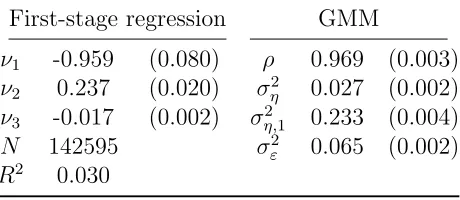
As in Heathcote et al. (2010), second-order autocovariances are used because observations only occur every two-years after 1995. In total, 292 moments identify the 4 shock process parameters, and I use the optimal GMM estimator.
First-stage regression GMM
ν1 -0.959 (0.080) ρ 0.969 (0.003) ν2 0.237 (0.020) ση2 0.027 (0.002) ν3 -0.017 (0.002) σ2η,1 0.233 (0.004) N 142595 σ2
ε 0.065 (0.002) R2 0.030
Table 1: PSID Estimation
Table 1 displays the parameter estimates. The first-stage regression coefficients imply mean labor efficiency declines 3% from age 24 to 30 (recall equivalized wages are used) and then grows steadily from age 30 to 64 for a total increase of 36%. The estimated shock process is highly persistent with parameters remarkably similar to those in Storesletten, Telmer, and Yaron (2004). This is despite a large number of differences, foremost being a different dependent variable.
4.2
Calibration
To use the estimated efficiency process parameters, I specify the the model efficiency process analogously to (9) and convert the annual estimates to three-year estimates. Specifically, I take ρ3 as the model persistence, (1 +ρ2 +ρ4)ση2 as the model persistent shock innovation variance,ση,12 as the model variance for z1, andσ2ε as the model variance for the i.i.d. shock.
This conversion gives that the three-year ahead forecast means and variances are the same in the model and data and that the initial variances are the same. Except for ν0 which is
used as a normalization constant, the age-profile parameters carry over directly. For retired households,
wherehR−1 = 63/10. The log(.5) term generates an exogenous 50% decline in labor efficiency
and is meant to capture reduced non-asset income in retirement.
Consistent with the theory, the persistent and transitory shocks are both discretized.18 The transitory shock is discretized using 3 points at 0 and ± 1 standard deviations. The persistent shock is discretized using 7 linearly-spaced points on an age-dependent grid that always covers 3 standard deviations (for retirees, the grid is the same as for R−1). The transition probabilities are computed using Tauchen (1986)’s method.
The labor grid is taken to be arbitrarily fine between 0.001 and 0.999 (one can think of the step size between grid points as being machine epsilon). The asset grid cannot be as fine since increasing the grid also increases the search space for the planner’s optimal policy. I use 50 strictly negative points and 250 points overall.
The utility function is chosen to be (cθ(1−n)1−θ)1−σ/(1−σ). The parameter σ is set to
1 + 1/θ so that constant relative risk aversion, 1−θ(1−σ), equals 2 for any calibrated value of θ. The risk-free price ¯q is set to give a 2% annual real interest rate.
For welfare comparisons, I specify an ex ante welfare function where α1(a = 0, e) = πe
for all e and αt(a, e) = 0 for all other a, e, t (and so the planner seeks to maximize welfare
of newborn households). This has been the most common choice in the literature for life-cycle models featuring default.19 This welfare measure accounts for the welfare of older households because V1(a = 0, e) implicitly values utility at all future states reached with
positive probability.
For comparison with the optimal policy and determining the remaining parameter values, I attempt to capture the current U.S. bankruptcy system and the value of informal default. In the U.S., any household in good standing can file for bankruptcy, so I setDt(a, e, n) = {0,1}
for alla, e, n, t. Since a bankruptcy stays on credit reports for 10 years, I setλt= 0.7 (for all t) to match this duration. Filing costs in the U.S. are comprised of two main components, official filing fees and attorney costs. Official Chapter 7 bankruptcy filing fees in 2016 were $335 dollars but can be waived for debtors earnings less than $150 below the poverty level (U.S. Courts, 2016). Attorney’s fees, which presumably are increasing in labor efficiency, are substantial. White (2007) states that a “typical” debtor’s cost of filing is between $1,800 and $2,800 (p. 192). So, I parameterize ζt(a, e, n) to allow for progressive costs ¯ζe. The slope
coefficient ¯ζ is then chosen to give average filing costs equal to 1% of average earnings. This
18The grids used in the computation are such that (ε, z) can always be recovered frome. That is,e=f(ε, z)
is invertible, which is required to be perfectly consistent with the theory. Although one can construct examples wheref is not invertible, there is always an arbitrarily small perturbation off that is invertible (a proof of this is available by request).
19For instance,Livshits et al.(2007),Athreya et al.(2009a), andGordon(2015) all use this. While testing
is based on an $1,800 filing cost as a fraction of 3 years of earnings at $60,000. The psychic costs κ(e) are parameterized as max{0, κ0+κ1zi,t+κ2εi,t}.
Informal default is modeled as autarky with an additional psychic cost κO≥0 in the first
period, which makes VO
t (a, e) = VtA(a, e)−κO.20 The cost κO is meant to capture all costs
associated with informal default such as phone calls from creditors and wage garnishments (with the maintained assumption that all collection efforts have a zero net recovery rate). For approximating the current U.S. system, I treatκOas a parameter and calibrate it. Later in this section I will treat κO as the planner’s policy instrument γ (recall γ influences the outside option value) and assume the planner can make κO arbitrarily large. In the next section, I will assume the planner can only choose κO= 0.
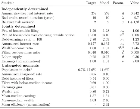
The 8 parameters (β, θ, ν0, κ0, κ1, κ2, κO, ζ) are used to match 8 moments from the data.
The discount factor β is primarily used to match a wealth-income ratio of 1 based on an annual ratio of 3. The Cobb-Douglas utility weight θ is used to match the fraction of hours spent working. In the PSID sample with age restrictions but no restriction on hours worked, the fraction of potential work time spent working is 27.6%. (This estimate assumes 16 hours of work time a day with 365 work days available per adult.) The earnings process parameter
ν0 sets average earnings to 1, a normalization. The psychic cost parameters κ0, κ1, κ2 are
used to match a debt-income ratio of 0.028, a filing rate of 1.20%, and an annualized interest rate of 12.7%. The first number is a triennial conversion of the annual number in Livshits et al.(2007), the filing rate is based on Chapter 7 and 13 personal bankruptcy filings relative to the working age population in 2015 converted to a triennial rate, and the last is from
Gordon (2015). The proportional filing cost parameter ζ is used to match a filing cost-earnings ratio of 0.01. Thinking of the outside option as an absorbing state with debts in permanent collection, the psychic cost of informal defaultκO is used to target the percent of
consumers with a third-party collection. In the past decade this has varied from 12 to 15% (FRBNY, 2017), and I use 13% as a target. The calibrated parameters and moments are given in Table 2.
The model delivers every targeted moment with mixed performance for the untargeted moments. The population in debt is in the range of 6.7% (Chatterjee et al.,2007) and 17.6% (Wolff, 2010), the former measuring strictly negative debt positions and the latter weakly negative. The annualized charge-off rate is about twice what it should be, but the implied model rate is closely linked to the interest rate because there are no transaction costs.21 As
20To be precise, once a household chooses the outside option, their policies are as if in autarky. That is,
their policies are the optimal policies corresponding to (2) with a= 0 in the first period and whatever is implied by the autarky policies and shocks thereafter. Consequently, VO
t (a, e) = Xt(0, e)−κ(e)−κO for a <0. By definition,VA
t (a, e) :=Xt(0, e)−κ(e) fora <0, soVtO(a, e) =VtA(a, e)−κO.
is typically the case for a normally distributed efficiency process, the model under-predicts earnings and wealth inequality.
The model’s implied psychic costs are increasing in both persistent and transitory earn-ings with a median value of 1.06. This median value is very large, around 16% in terms of consumption equivalent variation for a newborn, and consequently households with above-median earnings default very infrequently. However, the psychic costs quickly go to zero for households with negative shocks. E.g., for a transitory shock one-standard deviation below its mean, εit =−0.25, the psychic cost is zero if zi,t is zero.
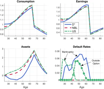
Figure 1 plots life-cycle profiles for consumption, earnings, asset holdings, and default rates (both bankruptcy filing rates and outside option take-up rates). In the data, bankrupt-cies are most frequent among 30-47 year olds (Livshits et al., 2007, Figure 1, p. 404). The model captures this but is too extreme with essentially no one filing for bankruptcy after age 45. Older households prefer the outside option because they have little need to borrow in retirement, which makes going to autarky (with the additionalκO cost) relatively less costly.
4.3
Baseline cases
Before analyzing the full optimal policy, it is useful to consider some baseline cases. The first baseline is the current U.S. system (referred to as US). The second is a zero borrowing limit (ZBL) economy where qt(a, e) = 0 for all a < 0, e, t, which provides a lower bound
on utility. A third baseline case is a natural borrowing limit (NBL) economy, which has
Dt(a, e, n) = {0}for all states. The last baseline must, by Corollary 1, improve on the NBL
economy. This policy specifies Dt(a, e, n) = {0} for all states having VtR(a, e) < VtO(a, e) or VR
t (a, e) undefined. I refer to this as the D
{} economy. For all the policies except US, I take
κO arbitrarily negative to focus on what optimal bankruptcy policy can achieve if informal
default can be made very costly (κO= 0 will be taken up in Section 5).
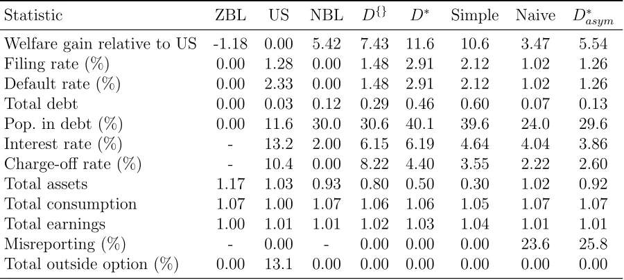
The results for ZBL, NBL, US, andD{}are summarized in Table 3. The reported welfare gain is the consumption equivalent welfare measure relative to US. ZBL is worse than US with a welfare loss of 1.2%. NBL on the other hand does much better with a welfare gain of 5.4%. Comparing the amounts of debt in US and NBL, debt is roughly 4 times larger in NBL. These findings agree with a large literature that has found the NBL does much better than model economies calibrated to match U.S. data moments because improved credit allows households to self-insure well. Figure 1 shows NBL increases consumption of young households relative to US, reducing savings early in life. Front-loading consumption improves welfare since β/q¯is significantly less than 1.
Statistic Target Model Param. Value
Independently determined
Annual risk-free real interest rate 2% 2% q¯ 0.942 Bad credit record duration (years) 10 10 λ 0.7
Relative risk aversion 2 2 σ 1 + 1/θ
Jointly determined
Pct. of households filing 1.20 1.28 κ0 1.06
Pct. of households ever choosing outside option 13.00 13.10 κO 0.008 Debt-earnings ratio × 100 2.80 2.69 κ1 1.23
Annualized interest rate 0.127 0.132 κ2 5.72
Wealth-income ratio 1.00 1.01 β1/3 0.945
Filing cost-earnings ratio 0.010 0.010 ζ¯ 0.008
Labor supply 0.28 0.27 θ 0.36
Earnings (normalization) 1.00 1.01 ν 2.03
Untargeted moments
Population in debt* 6.7%-17.6% 11.6% Annualized charge-off rate 0.05 0.10 Debt-income of filers 0.54 0.90 Filers with below-median income 0.69 1.00
Earnings gini 0.61 0.50
Wealth gini 0.80 0.72
Mean-median earnings 1.57 1.51
Mean-median wealth 4.03 2.46
Mean efficiency (normalization) - 2.92
Note: Model income is measured as en+ (1/q¯−1)a and “in debt” is a <0.
Statistic ZBL US NBL D{} D∗ Simple Naive D∗asym
Welfare gain relative to US -1.18 0.00 5.42 7.43 11.6 10.6 3.47 5.54 Filing rate (%) 0.00 1.28 0.00 1.48 2.91 2.12 1.02 1.26 Default rate (%) 0.00 2.33 0.00 1.48 2.91 2.12 1.02 1.26 Total debt 0.00 0.03 0.12 0.29 0.46 0.60 0.07 0.13 Pop. in debt (%) 0.00 11.6 30.0 30.6 40.1 39.6 24.0 29.6 Interest rate (%) - 13.2 2.00 6.15 6.19 4.64 4.04 3.86 Charge-off rate (%) - 10.4 0.00 8.22 4.40 3.55 2.22 2.60 Total assets 1.17 1.03 0.93 0.80 0.50 0.30 1.02 0.92 Total consumption 1.07 1.00 1.07 1.06 1.06 1.05 1.07 1.07 Total earnings 1.00 1.01 1.01 1.02 1.03 1.04 1.01 1.01 Misreporting (%) - 0.00 - 0.00 0.00 0.00 23.6 25.8 Total outside option (%) 0.00 13.1 0.00 0.00 0.00 0.00 0.00 0.00
Note: Interest and charge-off rates have been annualized; Misreporting is the rate conditional on filing; Total assets are measured as R a(1−max{d, o})dµ (capital in general equilibrium).
Table 3: Welfare and Allocations from Differing Default Policies
D{} generates a 7.4% welfare gain relative to US, 2 percentage points larger than NBL’s gain. While Corollary 1 shows D{} must weakly outperform NBL, quantitatively there is a sizable difference. This is despite D{} and NBL differing only in states where households cannot repay, in which caseD{}provides a fresh start and NBL does not. While implementing NBL would be very costly (probably involving a return to debtors’ prisons), implementing
D{} would be much less costly: Courts would determine whether a household could repay and, if not, give them a fresh start.
4.4
The optimal bankruptcy rule
The full optimal policy, labeled D∗, is now considered. It is computed using a genetic al-gorithm and multigrid on a super computer with the household problem solved six million times. Interested readers may consult AppendixB for more details.
As can be seen in Table 3,D∗ generates a 11.6% welfare gain relative to US, more than doubling NBL’s 5.4% gain. To see why the welfare gain is so large, first note that relative to US,D∗ generates 15 times more debt and, despite this, similar default rates with 50%lower
30 40 50 60 70 80 0.8
0.9 1 1.1 1.2 1.3 1.4
Consumption
30 40 50 60 70 80 0.4
0.6 0.8 1 1.2 1.4 1.6
Earnings
D* NBL US
30 40 50 60 70 80
Age
0 1 2
3 Assets
30 40 50 60 70 80
Age
0 0.02 0.04 0.06 0.08
Default Rates
Bankruptcy
Outside Option
Figure 1: Life-cycle Profiles for D∗, NBL, and US
positive average asset positions throughout the life-cycle. D∗’s larger debt amounts in mid-life increase labor through a negative wealth effect on leisure, which results in households working more when their labor efficiency is highest. As a result, average earnings are 2% larger in D∗ than in US (as can be seen in Table 3).
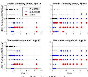
The optimal policy improves consumption smoothing by allowing bankruptcy only for those who benefit the most from it. This can be seen in Figure 2, which plots the optimal policy for select ages. A black dot means that the state is visited in equilibrium with prob-ability greater than 10−5. A blue plus sign means that the household files for bankruptcy if
the planner lets them, i.e.,dt(a, e) = maxDt(a, e, n). A red circle means Dt(a, e, n) = {0,1},
and so the household defaults. These parts of the policy are the most meaningful because changing the policy from {0,1} to {0} has a direct effect on default decisions and the plan-ner’s objective function (by virtue of ex ante welfare and the probability being greater than 10−5). The horizontal axis is debt (recall average earnings are roughly 1), and the vertical axis gives the standard deviations from the persistent shock mean. The top and bottom panels present the policy for the median and worst transitory shock values, respectively.
probabil-0 0.5 1 1.5 2 2.5 -3 -2 -1 0 1 2 3
Stdev from persistent mean
Median transitory shock, Age 30
Pr>.00001 & d=maxD & d=1
0 1 2 3 4 5
-3 -2 -1 0 1 2
3 Median transitory shock, Age 51
0 0.5 1 1.5 2 2.5
Debt -3 -2 -1 0 1 2 3
Stdev from persistent mean
Worst transitory shock, Age 30
0 1 2 3 4 5
Debt -3 -2 -1 0 1 2
3 Worst transitory shock, Age 51
Figure 2: The Optimal Policy by Age
ity. In this sense, the planner only allows default for the most unlucky households. Re-stricting default to only a small fraction of households is important because default rates effectively act as a borrowing tax: Borrowing interest rates relative to risk-free rates are 1/(1−Ee0|e,tdt+1(a0, e0)) or roughly Ee0|e,tdt+1(a0, e0) for small default rates; hence, a x%
de-fault rate translates (roughly) into a borrowing tax ofx%. The optimal policy mitigates this distortion by restricting default to those who benefit the most from it.
Interestingly, the optimal policy changes little in response to a negative transitory shock. This can be seen in comparing the median transitory state (the top panels) with the worst transitory state (the bottom panels). While it is true that more people wish to file in response to the negative transitory shock, the planner generally does not let them (i.e., a negative transitory shock creates more blue plus signs but not many more red circles).
The optimal policy responds more to persistent shocks than transitory shocks because the latter are easily insured using credit while the former are not. Because transitory shocks have no impact on future earnings, a negative shock hitting an aget household has no impact on
qt(a0, e). Hence, households can readily borrow to smooth out this small reduction in lifetime
income. In contrast, persistent shocks are much harder to self-insure via credit. Not only do they reduce lifetime income by a substantial amount, they also reduceqt(a0, e), which makes
offer bankruptcy in response to a negative persistent shock than a negative transitory one.
Livshits et al.(2007),Athreya et al.(2009b), and others have shown that high-bankruptcy-cost regimes are more preferable when shocks are less persistent and conversely for low-high-bankruptcy-cost regimes. The optimal policy—by treating persistent and transitory shocks differently—can have the best of both worlds, requiring households to self-insure against transitory shocks but allowing bankruptcy for insurance against persistent ones.
5
Constraints on the optimal policy
The optimal bankruptcy policy vastly improves welfare. However, the 11.6% welfare gain is an upper bound because of three constraints on optimal policy. The first constraint is that the policy should be simple enough for households and creditors to understand. The second con-straint is asymmetric information with moral hazard: By tying debt forgiveness to particular efficiency levels, the optimal policy under asymmetric information incentivizes households to misreport their efficiency status. The third constraint is limited commitment induced by an attractive outside option. This section explores how much each of these constraints affects the optimal policy.
5.1
Simple implementation
While the optimal policy is intuitive, implementing the optimal rule in practice would be challenging. It requires that households and creditors have intricate knowledge about not just efficiency processes, but about every aspect of bankruptcy law. This subsection looks for a parsimonious parameterization ofDt(a, e, n) that comes close toD∗ in terms of welfare.
Of course, the parameterization should be able to capture much of the optimal policy’s variation in the relevant region of the state space, which is the set ∆ =
{(a, e, t)|VD
t (a, e)> VtR(a, e) or VtR(a, e) infeasible}. For any state in ∆, households choose dt(a, e) = maxDt(a, e, n) and so changing Dt(a, e, n) from {0,1} to {0} or vice versa leads
to a direct effect on default decisions. Such a change will also have a direct effect on planner welfare to the extent the state is visited in equilibrium. After some experimentation, the logit regression
P r(maxDi,t = 1) = 1/(1 + exp(−δi,t)),
δi,t =b0+b11[agei,t ≥40] +b2log(−ai,t) +b3z˜i,t +b4ε˜i,t+i,t
˜
zi,t =zi,t/Stdev(z|t),ε˜i,t =εi,t/Stdev(ε)
(11)
condi-tioning on ∆ and weighting by the invariant distribution (recall z and ε give the persistent and transitory efficiency shocks, respectively). Consequently, a natural parameterization of
Dt(a, e, n) is (11) with rounding:
maxDt(a, e, n) = (
1 if b0+b11[age(t)≥40] +b2log(−a) +b3z˜t+b4ε > .˜ 5
0 otherwise . (12)
To ensure (12) is in fact parsimonious, the theoretical result that bankruptcy be al-lowed when repayment is infeasible is not used, i.e., (12) applies in all states. The op-timal parameters, found via a global maximization algorithm, are (b0, b1, b2, b3, b4) =
(−8.45,−1.95,6.48,−3.55,0.01).
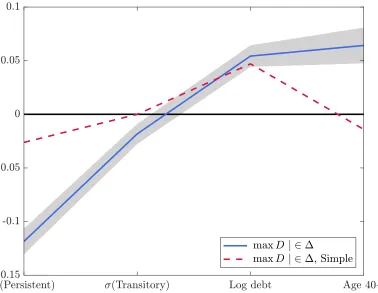
Figure 3: Average Marginal Effect on P r(maxD|∆)
Figure 3.22 The simple rule responds less to persistent shocks: A negative three standard deviation persistent shock increases the probability of filing by only around 8 percentage points compared to 36 points under D∗. The effect is even more extreme for transitory shocks, and the magnitude for the age dummy is also smaller. The simple rule is also slightly less sensitive to debt thanD∗. Overall, the best simple rule seems to be less responsive to a household’s state and offer less debt forgiveness.
With the simple rule, the planner is balancing two types of error. First, some households who would optimally be allowed to default will not be. This error results in too much in-tertemporal smoothing and too little intratemporal. Second, some who would optimally be prevented from defaulting are permitted. This results in the opposite case, too little intertem-poral smoothing and too much intratemintertem-poral. The results suggest the second type of error is worse: The planner should bias policy towards having too little default and too much credit. One benefit of doing this is that households can increase their own current consumption in a marginal fashion through debt issuance. In contrast, for the planner to increase a house-hold’s consumption by allowing for bankruptcy, the househouse-hold’s consumption must increase in a discrete fashion. By erring on the side of credit, the planner is effectively delegating consumption smoothing, reducing the cost of credit to help households better self-insure.
5.2
Asymmetric information with moral hazard
A second constraint on the optimal policy comes from asymmetric information with moral hazard. Since the optimal policy ties debt forgiveness to particular efficiency levelse, a valid concern is that a household might be able to manipulatee—which the model assumes to be exogenous—in order to obtain debt forgiveness. For instance, one might take a low paying job, request a lower wage, or even reduce human capital accumulation.
To capture this incentive, I allow households to effectively misreport their efficiency level. As before, I assume that the planner can observe hours worked n and earnings. However, I now take earnings to bexenwheree is a household’s potential labor efficiency andx∈[0,1] is a household’s “effort.” In a reduced form way, this effort captures the various means a household has of reducing their earnings xenbelow their “potential earnings”en. Note that
x > 1 is not permitted, which is a way of saying firms cannot be tricked into paying more than a household’s potential earnings (but presumably are more than happy to pay less). Hence, planner policy may depend on assets a, age t, labor n, and the observed efficiency
22Theoretically, the average marginal effects from (12) should be zero since a marginal change in a regressor
level ˜e=xe(earningsxendivided by time workedn), but may not depend on true efficiency
e, which is private information.23
To simplify the analysis, I assume that whenever the planner observes a wage ˜e /∈ E
(whereEis the finite support ofe), he does not permit bankruptcy (known lying is punished). Hence, household’s will always choose xso that ˜e∈E. Further, I assume the planner’s only policy instrument is to decide whether bankruptcy is allowed for each (a,˜e, t) ∈ A×E × {1, . . . , T}, and I denote it Dt(a,e˜). This assumption is not without loss of generality. In
particular, the planner could always do weakly better by using a direct mechanism featuring truth-telling. However, this restriction is advantageous for four reasons. First, it allows for a direct comparison withD∗. Second, the misreporting and welfare caused by naively applying
D∗ indicates how much this type of asymmetric information and moral hazard matters. Third, as argued in the introduction, it is unlikely that the constrained efficient allocation could be implemented using only bankruptcy. Last, solving the problem can be done with the same algorithm as in the benchmark, presumably making any computational errors comparable.
With these assumptions, the household problem can be written as
Vt(a, e) = max o,d,x∈[0,1]oV
O
t (a, e) +dVtD(e, x) + (1−o)(1−d)VtR(a, e, x)
s.t. xe∈E, d∈Dt(a, xe), o ∈ {0,1}, od= 0
(13)
where
VtR(a, e, x) = max
a0∈A,n∈Nu(c, n) +β X
e0
πee0|tVt+1(a0, e0)
s.t. c+qt(a0, e)a0 =xen+a, c > 0
(14)
and the value of bankruptcy is
VtD(e, x) = max
a0∈A,n∈Nu(c, n)−κ(e) +β X
e0
πee0|tVt+1(a0, e0)
s.t.c+ ¯qa0 =xen, c >0, a0 ≥0
(15)
Here, I have assumed that creditors can observe (or perfectly infer) the true wage per effi-ciency unit, focusing only on the asymmetric information problem bankruptcy courts face.24
23This particular type of moral hazard is costly for households. One could alternatively imagine that
households have the ability to earn the same amount but be paid “under the table” so that their earnings are unobservable (in this case, they would also need to hide consumption and/or assets to prevent earnings from being inferred). Adding this friction would further reduce the welfare gains achievable by bankruptcy policy.
24This is without loss of generality ifqt(a0, e) = ¯qP
e0πee0|t(1−max{dt+1(a0, e0), ot+1(a0, e0)}) is increasing
As a consequence, conditional on repayment, households always chooses full effort, x = 1. Equilibrium pricing is as before,qt(a0, e) = ¯qPe0πee0|t(1−max{dt+1(a0, e0), ot+1(a0, e0)}). The
planner solves
max
D X
a,e,t
αt(a, e)Vt(a, e)
s.t. Dt(a,˜e)∈ {{0,1},{0}} ∀a,e, t,˜
(16)
where Dt(a,˜e) depends on observed efficiency ˜e (not the true efficiencye).
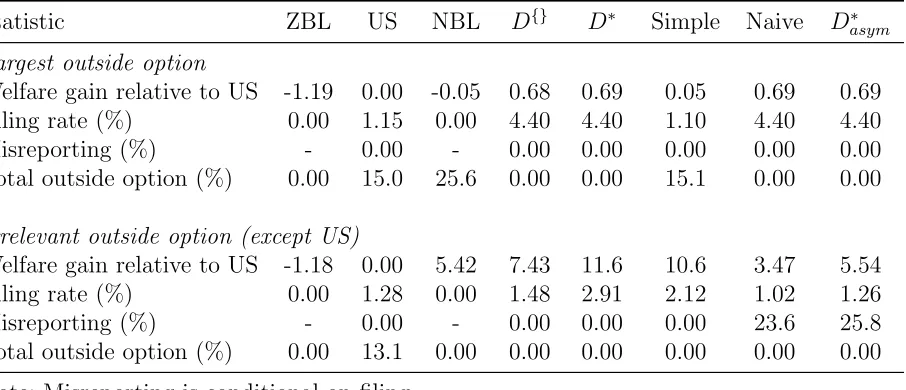
Table3reports two outcomes under asymmetric information. The column labeled “Naive” gives the outcome of applying the full information optimal policy (D∗) in the asymmetric information case without modification. Relative to D∗ in full information, the welfare gain goes from 11.6% down to 3.5%, debt goes down 85%, and filing rates decline.25 Conditional on default, 24% of households are misreporting their efficiency level to be eligible for dis-charge. Relative to such a policy, NBL is clearly better: NBL’s policy of never allowing bankruptcy means it induces no moral hazard and so delivers the same welfare gain as in the full information case, 5.4%.
Table 3also reports, in the column labeled D∗asym, the outcome from the optimal policy constructed under asymmetric information. While the welfare produced is slightly higher than that of NBL (5.5% versus 5.4%), in most respects the statistics look like those of NBL. Conditional on filing, the misreporting rate is 26%, and the overall default rate (1.26%) is about half that under US (2.33%). These results show the optimal policy in the presence of moral hazard is close to a natural borrowing limit economy, albeit allowing a small amount of default. However, as the next section will establish, this result hinges onVO being irrelevant.
5.3
Limited commitment
The third constraint on optimal policy is limited commitment in terms of an attractive outside option. Until now, I have assumed the planner can make κO large enough that VO
is irrelevant. I now consider the polar opposite case, restricting κO = 0 and thereby having
VO = VA, the maximum allowed by the theory. Because the psychic costs of default are positive for some households, Proposition 8 does not apply and debt can be supported in equilibrium. Table 4 reports the welfare under ZBL, US, NBL,D{}, D∗, Simple, Naive, and
thereby justifying the pricing of qt(a0, e). However, in general it is not possible to guarantee this without special assumptions such as an i.i.d. efficiency process (quantitatively unpalatable) or restricting policy to ensuredt(a, e) is decreasing inefor alla, t. If the true efficiency cannot be observed, one could in principle solve for equilibrium prices as inAthreya et al.(2012b), but practically speaking this is too costly here.
25The welfare gain is still measured relative to US under full information. This is not completely appropriate
D∗asym when VO=VA (all but the last two are computed assuming full information).
With limited commitment, US now slightly outperforms “NBL,” i.e., Dt(a, e, n) = {0}
<