Asymmetric Business Cycles and Sovereign Default
∗
Grey Gordon
†Pablo A. Guerron-Quintana
‡August 8, 2017
Abstract
What accounts for asymmetric (negatively skewed) business cycles in emerging economies? We show the asymmetry is tied to default risk and that a sovereign default model delivers negative skew.
Keywords: Skewness, Asymmetry, Business Cycles, Default
JEL classification numbers: F34, F41, F44
1
Introduction
Business cycles in emerging economies are characterized by high volatility, output being smoother
than consumption, and recurrent default episodes. A lesser known feature is that business cycles
in these countries are asymmetric, with recessions being more pronounced and lasting longer than
in small developed economies.
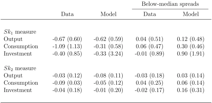
This asymmetry can be seen in Table 1, which gives the skewness for output, consumption,
and investment averaged over five emerging economies that have defaulted in recent history (the
data are described in the appendix). The standard skewness measure, Sk1, finds negative skew in
output, consumption, and investment. The other skewness measure, Sk2, which is more robust to
outliers (Kim and White, 2003), still shows negative skew in all three categories.1
The negative skew in the data is closely tied to default risk, and this can be seen in three ways. One way is to look at a subsample where spreads are below-median and thereby exclude
periods of high default risk and post-default periods. When doing this, the negative skew essentially
disappears as Table 1shows. A second way is to look at the relationship of spreads and skewness
∗We thank the referee for helpful comments and Diogo Lima for providing us with the EMBI and EMBI+ data.
Any mistakes are our own.
†Indiana University, [email protected]. ‡Boston College and ESPOL,[email protected].
1This measure is defined asSk
2=µ−σQ2, whereµis the mean,Q2is the median, andσis the standard deviation.
Below-median spreads
Data Model Data Model
Sk1 measure
Output -0.67 (0.60) -0.62 (0.59) 0.04 (0.51) 0.12 (0.48) Consumption -1.09 (1.13) -0.31 (0.58) 0.06 (0.47) 0.30 (0.46) Investment -0.40 (0.85) -0.33 (3.24) -0.01 (0.89) 0.90 (1.91)
Sk2 measure
Output -0.03 (0.12) -0.08 (0.11) -0.03 (0.18) 0.03 (0.14) Consumption -0.09 (0.03) -0.05 (0.12) 0.04 (0.25) 0.06 (0.14) Investment -0.04 (0.18) -0.01 (0.20) -0.02 (0.17) 0.16 (0.31)
Note: Statistics are computed using de-trended series, see the appendix for details; standard deviations are in parentheses; the data here are for Argentina, Ecuador, Mexico, Peru, and the Philippines.
Table 1: Skewness Statistics in the Data and Model
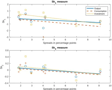
across countries. Figure 2does this for eight emerging economies (five high-spread and three low-spread), plotting the data along with best fit lines. There is a clear negative correlation between
spreads and skew for every measure. A third way to see the connection between negative skew
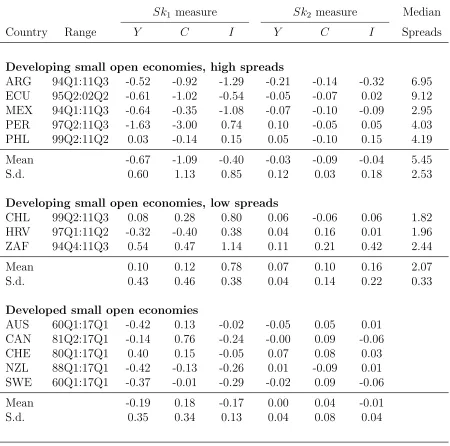
and default risk is to consider that developed small open economies (SOEs) have small or positive
skew. For instance, the averageSk1(Sk2) measure for the five developed SOEs in our sample range
from −0.19 to 0.18 (−0.01 to 0.04) depending on whether one looks at output, consumption, or
investment.
In the next sections, we lay out a SOE real business cycle (RBC) model with default that
delivers asymmetric business cycles. Crucially, it does so for normally-distributed productivity
shocks, i.e., there is no skewness in the underlying stochastic process. We then show how default and default risk drive the asymmetry. Intuitively, times of average or above-average productivity in
the model are as in any other RBC model. However, when productivity falls significantly, economic
activity declines for two reasons: the standard RBC reasons and increased debt-service costs.
Moreover, if default occurs, default costs lower productivity, which severely depresses consumption,
investment, and output. The reduced investment in default also depletes the capital stock, which
prolongs the recession. Consequently, the effects of upward movements in productivity have a
limited and short-lived impact while downward movements can have a drastic and long-lived
impact. This asymmetry results in an endogenous negative skew of consumption, investment, and
1 2 3 4 5 6 7 8 9 10 Spreads in percentage points
-3 -2 -1 0 1 2
Sk
1
Sk1 measure
Output Consumption Investment
1 2 3 4 5 6 7 8 9 10
Spreads in percentage points -0.4
-0.2 0 0.2 0.4 0.6
Sk
2
Sk2 measure
Figure 1: Skewness and default-risk spreads
2
Model and calibration
We briefly describe our model and calibration. For a more full description, seeGordon and
Guerron-Quintana (2017).
2.1
Model
In the long tradition of sovereign default models (Eaton and Gersovitz, 1981; Arellano, 2008;
Mendoza and Yue, 2012), a sovereign borrows in international markets to maximize the welfare of
domestic residents. The residents have consumptionc, supply laborl, and rank consumption/labor
bundles according to aGreenwood, Hercowitz, and Huffman(1988) period utility functionu(c, l) = (c−ηlω
ω)
1−σ/(1−σ) with discount factor β. The sovereign produces output y using capital k and
labor l according to y = Akαl1−α. Productivity follows logA0 = (1−ρ
A) logµA+ρAlogA+ε0A,
where εA ∼N(0, σA2).
The sovereign has access to long-term debt contracts in which outstanding debt matures at
a rate λ. Debt not maturing pays a coupon z. The sovereign’s stock of debt is denoted −b (the
literature uses b as assets by convention). New bond issuance is given by −b0+ (1−λ)b, which is
discounted by a price q.
from credit markets (i.e., goes to autarky). Third, it remains in autarky with probability 1−φ.
Last, for the duration of autarky, a fraction κ(A) of output is lost.
The sovereign’s problem is to solve
V (b, k, m, A) = max
d∈{0,1}(1−d)V
nd(b, k, m, A) +dVd(k, A),
whered is the default choice andVd(Vnd) is the value of defaulting (not defaulting). The variable
m is an i.i.d. endowment shock that aids computation. The value of not defaulting is
Vnd(b, k, m, A) = max
c,l,k0≥0,b0≤0u(c, l) +βEm0,A0|AV (b 0
, k0, m0, A0)
s.t.c+i+q(b0, k0, A)(b0−(1−λ)b) =Akαl1−α+m−Θ
2 (k
0 −
k)2+ (λ+ (1−λ)z)b
k0 =i+ (1−δ)k,
where i is investment and Θ controls the cost of adjusting capital. The value of defaulting or of
being in autarky is
Vd(k, A) = max
c,l,k0≥0u(c, l) +βEm
0,A0|A(1−φ)Vd(k0, A0) +φV(0, k0, m0, A0)
s.t.c+i= (1−κ(A))Akαl1−α−Θ
2(k
0 −
k)2
k0 =i+ (1−δ)k.
The equilibrium debt prices implied by risk-neutral foreign lenders who make zero profits
loan-by-loan (in expectation) are given by
q(b0, k0, A) =Em0,A0|A(1−d(b0, k0, m0, A0))
λ+ (1−λ) [z+q(b00, k00, A0)]
1 +r∗ ,
where b00=b0(b0, k0, m0, A0), k00 =k0(b0, k0, m0, A0), and r∗ is a risk-free international rate on a
one-period bond. Note that default risk, Em0,A0|Ad0, and spreads—an increasing function of 1/q—are
intimately linked.2
2.2
Calibration
We now summarize the calibration, which is the same as in Gordon and Guerron-Quintana(2017).
A period is a quarter. The coupon payment is 3% (z =.03) with 5% of debt maturing each period
(λ = .05), which nearly matches the Argentinean data’s 20 quarter median maturity of average
bonds and 11% value-weighted average coupon rate (Chatterjee and Eyigungor, 2012). Choosing
φ = 0.1, the average stay in autarky is 2.5 years. Following Neumeyer and Perri (2005), we
set ρA = .95, which is a value consistent with Fernandez-Villaverde, Guerron-Quintana,
Rubio-Ramirez, and Uribe, 2011 and much of the SOE business-cycle literature. Mean productivity µA,
the labor disutility parameterη, and depreciationδ are chosen so that, in the steady state without
foreign lending, output, labor, and the investment-GDP ratio equal 1, 1, and 0.05, respectively. The utility curvature σ is set to 2. The remaining parameters are chosen to match six moments
from Argentina’s data: the debt-output ratio −Eb/y, the average spreadEr, the spread volatility
σr, the volatility of investment σi, the volatility of output σy, and relative consumption volatility
σc/σy. InGordon and Guerron-Quintana (2017), we show this calibration delivers simultaneously
the business cycles and default properties of emerging economies such as Argentina.
3
Results and the model mechanism
To compute the model’s skewness statistics, we generate 20,000 simulations of length 75, which is
roughly the number of periods available for each of our developing SOEs. Of these, we keep only
the 14,101 simulations that had at least one default (in agreement with our sample selection for
countries).3 After logging and HP-filtering the model data, we compute the average and standard
deviation of the skewness measures, and these are reported in Table 1. On average, the model
delivers negative skew in output, consumption, and investment in both theSk1 andSk2 measures.
While the averages are all negative, the large standard deviations reflect it is possible to have
positive skew depending on the simulation. This agrees with the positive skew (depending on the
statistic) that can be found in Peru and the Philippines (see the appendix for a country-specific
breakdown).
As we argued in the introduction, the skewness in the data is driven by default risk, and this is
also true in the model. This can be seen in Table1, where—conditioning on below-median spreads
and hence low default risk—the negative skew disappears, just as in the data. Another way to see
this is that of the 5,899 simulations where a default did not occur, the Sk1 (Sk2) measures range
from −0.03 to 0.89 (−0.01 to 0.02) and so exhibit little or positive skew.
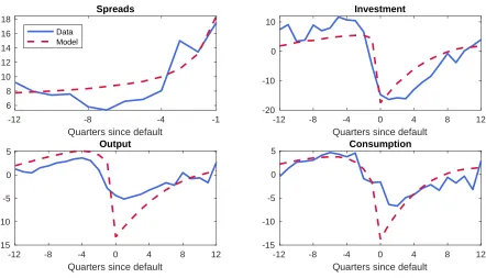
The mechanism producing negative skew can be seen in Figure2, which shows what happens, on
average, before and after a default. In the periods leading to a default, spreads are initially flat but
accelerate upwards in the year just before default. Perhaps surprisingly, investment, consumption
and output rise on average until a few quarters before default. But when spreads start to increase, this trend is reversed: Investment, consumption, and output begin to fall, gradually at first but
accelerating with a sharp collapse at default. The small movements up with larger and faster
movements down—the latter occurring in periods of high spreads and default risk—contribute to
negative skew. As the protracted recession after default is both an unusual (the average quarterly
default rate in the model is 1.3%) and severe period of economic activity, it also generates negative
3If this number seems small, note the model’s quarterly default rate of 1.3% should produce—if default occurred
-12 -8 -4 0 4 8 12
Quarters since default
-20 -10 0 10
Investment
-12 -8 -4 0 4 8 12
Quarters since default
-15 -10 -5 0
5 Consumption
-12 -8 -4 0 4 8 12
Quarters since default
-15 -10 -5 0
5 Output
-12 -8 -4 -1
Quarters since default
6 8 10 12 14 16 18
Spreads
Data Model
Figure 2: Investment Dynamics around Default
skew. The recession itself is triggered by low productivity and default costs, but it is protracted
because of a depleted capital stock due to investment that is up to 20% below trend.
Conditioning on periods where default risk is low, the model generates zero or positive skew. In
these periods, increases and decreases in productivity lead to changes in consumption, investment,
and output that are relatively small and persist at normal business cycle frequencies. In contrast,
when default risk is high, decreases in productivity cause rapid adjustments that—in the case
of a default—lead to severe and long-lasting recessions. Hence, default and default risk produce
negative skew in the model, just as they seem to in the data.
4
Conclusion
Our analysis shows that default and default risk significantly contribute to the negative skew seen
in developing small open economies.
References
C. Arellano. Default risk and income fluctuations in emerging economies. American Economic
Review, 98(3):690–712, 2008.
S. Chatterjee and B. Eyigungor. Maturity, indebtedness, and default risk. American Economic
J. Eaton and M. Gersovitz. Debt with potential repudiation: Theoretical and empirical analysis.
The Review of Economic Studies, 48(2):289–309, 1981.
J. Fernandez-Villaverde, P. Guerron-Quintana, J. Rubio-Ramirez, and M. Uribe. Risk matters:
The real effects of volatility shocks. American Economic Review, 101(6):2530–2561, 2011.
G. Gordon and P. Guerron-Quintana. Dynamics of investment, debt, and default. Review of
Economic Dynamics, Forthcoming, 2017.
J. Greenwood, Z. Hercowitz, and G. W. Huffman. Investment, capacity utilization, and the real
business cycle. American Economic Review, 78(3):402–417, 1988.
T. H. Kim and H. White. On robust estimation of skewness and kurtosis: Simulation and
appli-cation to the S&P500 index. Mimeo, 2003.
E. Mendoza and V. Yue. A general equilibrium model of sovereign default and business cycles.
Quarterly Journal of Economics, 127(2):889–946, 2012.
A. Neumeyer and F. Perri. Business cycles in emerging economies: The role of interest rates.
Journal of Monetary Economics, 52(2):345–380, 2005.
A
Data description and simulation details
National accounts data are collected from the International Financial Statistics and OECD’s
sta-tistical database. The national accounts variables are seasonally adjusted, real, logged and
HP-filtered with smoothing parameter 1600. Following Arellano (2008), the spreads are returns for
EMBI+ and EMBI Blended-Yield Maturity minus the 5-Year Treasury Constant Maturity Rate
(GS5 in FRED, averaged by quarter). Table2gives the time periods used for each country (for the emerging markets, we required spreads data to be available which restricts the sample somewhat).
Figure 2 is reproduced from Gordon and Guerron-Quintana (2017) and uses a slightly different
Sk1 measure Sk2 measure Median
Country Range Y C I Y C I Spreads
Developing small open economies, high spreads
ARG 94Q1:11Q3 -0.52 -0.92 -1.29 -0.21 -0.14 -0.32 6.95 ECU 95Q2:02Q2 -0.61 -1.02 -0.54 -0.05 -0.07 0.02 9.12 MEX 94Q1:11Q3 -0.64 -0.35 -1.08 -0.07 -0.10 -0.09 2.95 PER 97Q2:11Q3 -1.63 -3.00 0.74 0.10 -0.05 0.05 4.03 PHL 99Q2:11Q2 0.03 -0.14 0.15 0.05 -0.10 0.15 4.19
Mean -0.67 -1.09 -0.40 -0.03 -0.09 -0.04 5.45
S.d. 0.60 1.13 0.85 0.12 0.03 0.18 2.53
Developing small open economies, low spreads
CHL 99Q2:11Q3 0.08 0.28 0.80 0.06 -0.06 0.06 1.82 HRV 97Q1:11Q2 -0.32 -0.40 0.38 0.04 0.16 0.01 1.96 ZAF 94Q4:11Q3 0.54 0.47 1.14 0.11 0.21 0.42 2.44
Mean 0.10 0.12 0.78 0.07 0.10 0.16 2.07
S.d. 0.43 0.46 0.38 0.04 0.14 0.22 0.33
Developed small open economies
AUS 60Q1:17Q1 -0.42 0.13 -0.02 -0.05 0.05 0.01 CAN 81Q2:17Q1 -0.14 0.76 -0.24 -0.00 0.09 -0.06 CHE 80Q1:17Q1 0.40 0.15 -0.05 0.07 0.08 0.03 NZL 88Q1:17Q1 -0.42 -0.13 -0.26 0.01 -0.09 0.01 SWE 60Q1:17Q1 -0.37 -0.01 -0.29 -0.02 0.09 -0.06
Mean -0.19 0.18 -0.17 0.00 0.04 -0.01
S.d. 0.35 0.34 0.13 0.04 0.08 0.04
Note: Y, C,and I are output, consumption, and investment respectively; all data have been logged and HP-filtered; country codes are in ISO 3166-1 alpha-3 format.