Chapter V
Multivariate analysis...
Purpose of
Chapter
This chapter deals when more than two variables
simultaneously analyzed, for this chapter multivariate analysis
is used, such as multiple regression, partial correlation, logistic
regression model, etc.
Essentially,
multivariate analysis
is a tool to find patterns and
relationships between several variables simultaneously. It lets
us predict the effect a change in one variable will have on other
variables
.
5.1 Introduction
Multivariate analysis consists of a collection of methods that can be used when several measurements are made on each individual or object in one or more samples. We refer to measures as variables and to individuals or objects as units.
models and multivariate statistics. And with the high availability of high-speed computers and multivariate software, many users can address these questions through Multivariate Techniques.
Data Types
A single sample with several variables measured on each sampling unit (subject or object); or a single sample with two sets of variables measured on each unit; or two samples with several variables measured on each unit; or three or more samples with several variables measured on each unit.
Types of Measurements
Nominal: Categorical variables with no meaningful order (Examples: Gender, Hair color);
Ordinal: Categorical variables where a meaningful order exists (Examples: Social class, Rating of instructor);
Interval: Numerical variables where taking differences is meaningful, but there is no fixed zero position (Examples: Temperature using Celsius/Fahrenheit);
Ratio: Numerical variables where taking ratios is meaningful since there is a fixed zero (Examples: Age, Height, and Weight). Interval and Ratio are Metric data ⇒ this data can be manipulated mathematically.
Types of Multivariate Techniques:
1. Dependence techniques: a variable or set of variables is identified as the dependent variable to be predicted or explained by other variables known as independent variables.
2. Interdependence techniques: involve the simultaneous analysis of all variables in the set, without distinction between dependent variables and independent variables.
Classification of Multivariate Methods
5.2 Multiple Regression Analysis Technique • This technique is appropriate:
• Illustrative Research Question(s) this technique can answer:
Are sales significantly affected by advertising expenditures and price (where all three variables are measured in RWF)?
What proportion of the variation in sales is accounted by advertising and price?
How sensitive are sales to changes in advertising and price?
5.3 Partial correlation
The techniques of partial correlation can be used when a researcher wishes to observe how a specific bivariate relationship behaves in the presence of a third variable. By observing the partial correlation coefficients, we can identify direct or spurious and intervening relationship.
5.4 Logistic Regression Analysis
Logistic regression analysis is used to examine relationships between variables when the dependent variable is nominal, even though independent variables are nominal, ordinal, interval, or some mixture thereof. Suppose that one wanted to determine which program interventions were associated with a JOBS Program client's ability to get a job within six months of exiting the program. The outcome variable would be "job" or "no job” clearly a nominal variable. One could then use several independent variables such as job training, post-secondary education and the like to predict the odds of getting a job.
Sometimes we need to predict the variable that has only two possible values (a binary dependent variable). For example, will a Kigali bank customer choose online banking, or not?
The equation predicts the probability:
• Illustrative Research Question(s) this technique can answer:
Whether you are a market researcher who needs to make accurate predictions about new product launches, you can make reliable prediction.
How does the probability of getting lung cancer change for every additional pound of overweight and for every X cigarettes smoked per day?
Do body weight calorie intake, fat intake, and age have an influence on heart attacks (yes vs. no)?
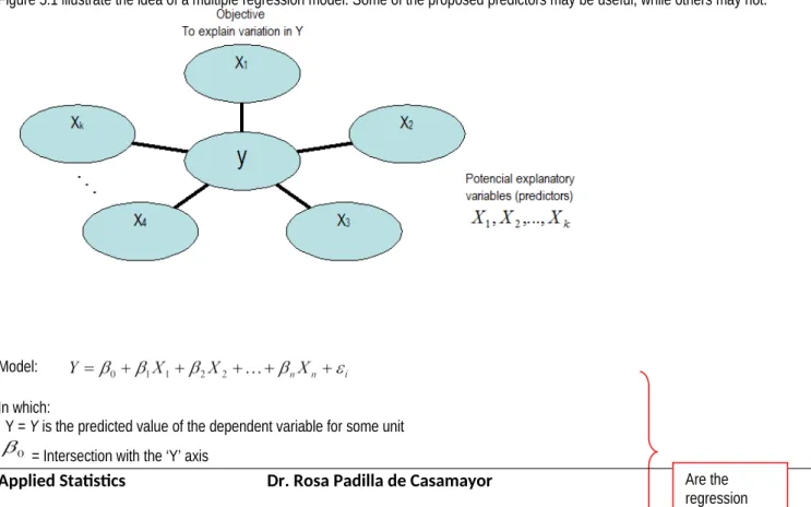
5.2 Analysis for Multiple Regression
Multiple linear regressions are an extension of the simple model that incorporates several independent variables (called predictors). Multiple regression analysis produces an equation with several coefficients, depending on the number of independent variables X are introduced to the model, thus generating hyper planes.
Figure 5.1 illustrate the idea of a multiple regression model. Some of the proposed predictors may be useful, while others may not.
Model:
In which:
Y = Y is the predicted value of the dependent variable for some unit = Intersection with the ‘Y’ axis
= The slope of ‘y’ with respect to the variable holding X2, X3,…Xp constant
= The slope of ‘y’ with respect to the variable holding X1, X3, …Xp constant
….
= The slope of ‘y’ with respect to the variable Xp keeping the variables constants. X1, X2, …, Xn are values on the independent variables
= Random error in Y for observation i
Assumptions
In Linear regression, the sample size is at least 20 cases per independent variable in the analysis.
The regression has five key assumptions:
Linear relationship. First, linear regression needs the relationship between the independent and dependent variables to be linear. It is also important to check for outliers since linear regression is sensitive to outlier effects. The linearity assumption can best be tested with scatter plots.
Multivariate normality. Multiple regression assumes that the residuals are normally distributed. The linear regression analysis requires all variables to be multivariate normal. This assumption can best be checked with a histogram or a PP-Plot. Normality can be checked with a goodness of fit test, e.g., the Kolmogorov-Smirnov test or Shapiro Wilk for small samples. When the data is not normally distributed a non-linear transformation (e.g., log-transformation) might fix this issue.
No or little multicollinearity. (Absence of correlation between two or more independent variables ‘generally in simple correlation 0.90 and above’. Multicollinearity in multiple regression analysis refers to how strongly interrelated the independent variables in a model are. When multicollinearity is too high, the individual parameter estimates become difficult to interpret. Most regression programs can compute variance inflation factors (VIF) for each variable. (Hair et al., 2006) recommend that a large VIF value (10 or above) or a very small tolerance value (0.10 or below) indicates high collinearity or multicollinearity.
If multicollinearity is found in the data, centering the data (that is deducting the mean of the variable from each score) might help to solve the problem. However, the simplest way to address the problem is to remove independent variables with high VIF values.
No auto-correlation. Linear regression analysis requires that there is little or no autocorrelation in the data. Autocorrelation occurs when the residuals are not independent from each other. The range of this statistic ranges from 0 to 4. A value around 2 means that errors are not correlated, less than 2 that the errors are positively correlated and greater than 2 that are negatively correlated. For instance, this typically occurs in stock prices, where the price is not independent from the previous price. (The Durbin-Watson d ≈ 2, i.e. when is between the two critical values of 1.5 < d < 2.5). Therefore, we can assume that there is no first order linear auto-correlation in our multiple linear regression data.
Homoscedasticity. This assumption means that the variance around the regression line is the same for all values of the predictor variable (X). The plot shows a violation of this assumption.
Example
Some film distributor’s offer discount cinema tickets via email. A random sample of 9 moviegoers is taken, and the number of movies the person has seen in the last year (Y), their age (X1) and income (X2), and the number of discount cinema tickets they have received via
email in the last year (X3), is recorded.
The data is used to develop a multiple regression model to predict the number of times an individual goes to the movies per year from their age, income and number of discount cinema tickets received. The following results are obtained.
Table 5.1. Association between Number of movies seen at a cinema last year, age, Income, and Number of emailed discount cinema
Number of movies seen
at a cinema last year (y) Age (X1)
Income (X2)
Number of emailed discount cinema tickets
received last year (X3)
10 42 30 3
8 50 30 2
12 27 55 4
11 29 50 3
14 30 60 4
15 25 58 5
7
11 5027 2047 23
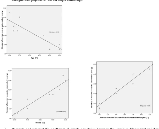
a. Draw the scatter diagram to see the trend and the relationship between the variables under study.
b. Compute and interpret the coefficient of simple correlation between the variables (dependent variable: number of movies the person has seen in the last year)
c. Compute and interpret multiple correlation coefficient, multiple coefficient of determination and assumption about Autocorrelation by Durbin Watson
d. Determine the multiple regression equation by performing an appropriate F test at =.05
e. Perform appropriate tests to determine the significance of the predictors. Use =.05 and show all working. f. Assumption about multicollinearity
g. Testing assumption of multivariate normality
Solution
a. Draw the scatter diagram to see the trend (linear or nonlinear) and the relationship between the variables under study (in the dialogue box graphics SPSS old single scattering).
Figure 5.2. Scatter plot for each predictor
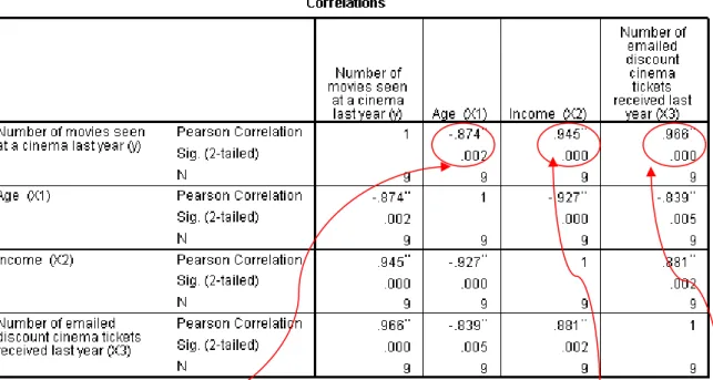
b. Compute and interpret the coefficient of simple correlation between the variables (dependent variable: number of movies the person has seen in the last year)
Interpretation: Number of movies seen at cinema last year has a strong direct association with Income and Number of emailed discount, while Age has a strong inverse association.
c. Compute and interpret multiple correlation coefficient, multiple coefficient of determination and assumption about Autocorrelation by Durbin Watson
Figure 5.4. Steps for Multiple Regressions in SPSS
Interpret the following Outcomes of SPSS software.
Figure 5.5. Model Summaryb
Model R R Square Adjusted R Square
Std. Error of the
Estimate Durbin-Watson
1
.987a .974 .959 .58251 2.023
a. Predictors: (Constant), Number of emailed discount cinema tickets received last year (X3), Age (X1), Income (X2) b. Dependent Variable: Number of movies seen at a cinema last year (y)
Multiple coefficient of correlation: R = .987 (the model improved by interacting independent variables), in other hand there are strong correlation between number of movies seen with number of emaildiscount, age and income.
Multiple coefficient of determination: R2 = .974. So 97.4% of the variation in the Number of movies seen at cinema last year can be
explained by the variation in the Number of cinema tickets sent by email discount received last year, the Age and the variation of Income. Assumption about Autocorrelated: Durbin Watson = 2.023 the residual are nonautocorrelated, because the value is close to 2.
(1.5 < d < 2.5), therefore assumption of non-autocorrelated assumed.
d. Determine the multiple regression equation by performing an appropriate F test at =.05 . Figure 5.6. ANOVAb
Model Sum of Squares df Mean Square F Sig.
1 Regression 64.526 3 21.509 63.387 .000a
Residual 1.697 5 .339
Total 66.222 8
a. Predictors: (Constant), Number of emailed discount cinema tickets received last year (X3), Age (X1), Income (X2)
b. Dependent Variable: Number of movies seen at a cinema last year (y)
Interpretation: As Sig < 0.05 then reject null hypothesis, indicating that at least one of the explanatory variables is related to number of movies seen at a cinema last year.
Hypothesis of Slope
Approach of the hypothesis:
(Consider that all the coefficients are simultaneously equal to zero)
(At least one regression coefficient is not equal to zero)
The rejection of the null hypothesis, indicating that at least one of the independent variables X1, X2, ..., Xk, contributes significantly to the
model and as such could be useful for estimating the mean of Y.
Method: Enter
As we can see, the variable number of discount cinema tickets sent by email last year, their income, these are significant in the amount of movies seen in a cinema last year.
The model has the following equation:
Figure 5.7. Coefficientsa
Model
Unstandardized Coefficients
Standardized Coefficients
t Sig.
B Std. Error Beta
1 (Constant) .430 3.345 .129 .903
Age (X1) .031 .053 .112 .581 .586
Income (X2) .093 .040 .511 2.311 .069
Number of emailed discount cinema tickets received last year (X3)
1.665 .417 .610 3.996 .010
a. Dependent Variable: Number of movies seen at a cinema last year (y)
(Number of emailed discount cinema tickets received last year the sig = .010<.05, indicating this variable is an important predictor) and income the sig = .069<.10, thus income has some influence as a predictor, but its effect is not as strong as the previous variable; in the same way we see the variable age has not influence as a predictor (sig=.586).
f. Assumption about multicollinearity
Interpretation
The variables do not show multicollinearity, because all tolerances are greater than .10 and VIF are less than 10.
g. Testing assumption of multivariate normality Ho: the residuals follow a normal distribution Ha: the residuals do not follow the normal distribution
Steps to perform assumption of normality
Output
Tests of Normality
Kolmogorov-Smirnova Shapiro-Wilk
Statistic df Sig. Statistic df Sig.
Unstandardized Residual .233 9 .171 .871 9 .128
a. Lilliefors Significance Correction
We check Shapiro Wilk because the sample size is small (less than 30)
Decision: We cannot reject null hypothesis because sig = .128 < .05, therefore we conclude that assumption assume, the residuals follow a normal distribution
Note:
1. Examine the model F-test. If the test result is not significant, the model should be dismissed and there is no need to proceed to further steps.
2. Examine the individual statistical tests for each parameter estimate. An independent variable with significant results can be considered a significant explanatory variable. If an independent variable is not significant, the model should be run again with no significant predictors deleted. Often, it is best to eliminate predictor variables one at a time, and then rerun the reduced model. 3. Examine the model R2. No cutoff values exist that can distinguish an acceptable amount of explained variation across all regression
In other words, the regression is run for pure forecasting purposes. When the model is more oriented toward explanation of which variables are most important in explaining the dependent variable, cutoff values for the model R2 are not really appropriate.
5.3 Partial Correlation
The technique of partial correlation can be used when a researcher wishes to observe how a specific bivariate relationship behaves in the presence of a third variable.
Figure 5.8 Types of Correlation
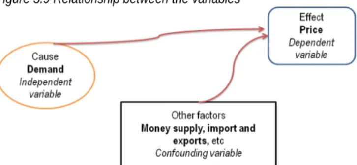
Generally, a large number of factors simultaneously influence all social and natural phenomena. For example, when we study the correlation between price as dependent variable and demand as independent variable), we completely ignore the effect of other factors like money supply, import and exports etc. which definitely have a bearing on the price.
Figure 5.9 Relationship between the variables
The correlation co-efficient between two variables X1 and X2, studied partially after eliminating the influence of the third variable, from both
of them, is the partial correlation coefficient.
The partial correlation analysis assumes great significance in cases where the phenomena under consideration have multiple factors influencing them, especially in physical and experimental sciences, where it is possible to control the variables and the effect of each variable can be studied separately.
Application example:
Why does voter turnout vary from election to election? For municipal elections in seven different cities of Africa, information has been gathered on the percent of registered voters who actually voted, unemployment rate, and the percentage of all political advertisements that used “negative campaigning” (personal attacks, negative portrayals of the opponent’s record, etc.). For the sake of convenience, the data for the three of the variables are presented again here along with descriptive statistics and Zero-order correlations.
Turnout Unemployment Rate % negative Ads.
Nairobi 70 10 48
Luanda 68 9 53
Lagos 71 10 40
Sierra Leone 55 5 60
Madagascar 60 8 63
Morocco 60 8 63
Mauritius 55 5 60
Mean 62.7143 7.8571 55.2857
Standard
Deviation 6.87300 2.11570 8.71233
Turnout Unemployment Rate % negative Ads.
Turnout .948** -.853*
Unemployment Rate
-.685 Types of Correlation
Direct and Inverse
Simple, Partial and Multiple
a. Compute the partial correlation coefficient for the relationship between turnout (Y) and unemployment (x) while controlling for the effect of negative advertising (Z). What effect does this control variable have on the bivariate relationship? Is the relationship between turnout and unemployment direct?
b. Compute the partial correlation coefficient for the relationship between turnout (Y) and negative advertising (x) while controlling for the effect of unemployment (Z). What effect does this have on the bivariate relationship? Is the relationship between turnout and negative advertising direct?
c. Find the unstandardized multiple regression equation with unemployment (X1) and negative ads. (A2) as the independent variables.
What turnout would be expected in a city in which the unemployment rate was 10% and 75% of the campaign ads were negative? d. Compute beta-weigths for each independent variable. Which has the stronger impact on turnout?
e. Compute the multiple correlation coefficient (R) and the coefficient of multiple determination (R2). How much of the variance in voter
turnout is explained by the two independent variables?
Solution
a. Compute the partial correlation coefficient for the relationship between turnout (Y) and unemployment (x) while controlling for the effect of negative advertising (Z). What effect does this control variable have on the bivariate relationship? Is the relationship between turnout and unemployment direct?
Correlations
Control Variable Turnout Unemployment_rate
% Negative
Advertising Turnout Significance (2-Correlation 1.000 .957
tailed) .003
df 0 4
b. Compute the partial correlation coefficient for the relationship between turnout (Y) and negative advertising (x) while controlling for the effect of unemployment (Z). What effect does this have on the bivariate relationship? Is the relationship between turnout and negative advertising direct?
Correlations
Control Variable Turnout % NegativeAdvertising
Unemployment_rate Turnout Correlation 1.000 -.879
Significance
(2-tailed) .021
df 0 4
For turnout (y) and % Negative Advertising (x) while controlling for Unemployment rate (Z), r = -.879. The bivariate relationship is not affected by the control variable, and also the relationship is not direct, this is an inverse relationship.
c. Find the unstandardized multiple regression equation with unemployment (X1) and negative ads. (X2) as the independent variables.
What turnout would be expected in a city in which the unemployment rate was 10% and 75% of the campaign ads were negative?
Coefficientsa
Model
Unstandardized Coefficients StandardizedCoefficients
t Sig.
B Std. Error Beta
1 (Constant) 61.955 6.659 9.304 .001
Unemployment_rate 2.226 .338 .685 6.590 .003
% Negative Advertising -.303 .082 -.384 -3.689 .021
a. Dependent Variable: Turnout
Turnout (Y) = 61.955 + (2.226) unemployment (X1) + (-.303) negative advertising (X2).
For unemployment (x1) = 10 and negative advertising (x2) = 75, then
The expected value for Turnout = 61.52
d. Compute beta-weights for each independent variable. Which has the stronger impact on turnout?
For unemployment (x1): ß1 = .685, for negative advertising (x2): ß2 = -.384, unemployment has a stronger effect on turnout than
negative advertising. Note that the independent variables’ effect on turnout is in opposite directions.
e. Compute the multiple correlation coefficient (R) and the coefficient of multiple determination (R2). How much of the variance in
voter turnout is explained by the two independent variables? Model Summary
Model R R Square Adjusted RSquare Std. Error of theEstimate
1 .988a .977 .966 1.27629
a. Predictors: (Constant), % Negative Advertising, Unemployment_rate
Multiple correlation coefficient: r = .988, there is a strong association between the participation rate with the % of negative publicity, and unemployment rate.
Coefficient of multiple determination: R2 = .977.
97.7 % of the variation in turnout is explained by the variation of negative publicity and the unemployment rate.
How much of the variance in voter turnout is explained by the two independent variables? In 97.7%.
5.4 Logistic Regression
Logistic regression data set is essentially the same as a multivariate regular linear regression data set except that the dependent “Y”variable is binary or any type of categorical variable.
Types of Logistic regression:
A binomial logistic regression (often referred to simply as logistic regression), predicts the probability that an observation falls into one of two categories of a dichotomous dependent variable based on one or more independent variables that can be either continuous or categorical. Alternatively, if you have more than two categories of the dependent variable, see multinomial logistic regression.
Multinomial Logistic regression: In this type of logistic regression, there are more than two outcomes. Banking business example: Bank wants to know what the probability is that particular customer will invest in Bank Deposit or Mutual fund or Bond.
Ordinal Logistic regression: In this kind of logistic regression, there are more than two outcomes and it should be in order. Banking business example: If bank run one customer satisfaction survey on customer service. Here bank tries to predict particular customer will give feedback as excellent or satisfactory or good or bad.
Assumption for used Logistic Regression
Assumption 1:
Dependent variable should be measured on a dichotomous scale. Examples of dichotomous variables include gender (two groups: "males" and "females"), body composition (two groups: "obese" or "not obese"), and so forth. However, if your dependent variable was not measured on a dichotomous scale, but a continuous scale instead, you will need to carry out multiple regression if your dependent variable was measured on an ordinal scale, ordinal regression would be a more appropriate starting point.
Assumption 2: You have one or more independent variables, which can be either continuous (i.e., an interval or ratio variable) or categorical (i.e., an ordinal or nominal variable). Examples of continuous variables include revision time (measured in hours), intelligence (measured using IQ score), exam performance (measured from 0 to 100), weight (measured in kg), and so forth. Examples of ordinal variables include Likert items (e.g., a 7-point scale from "strongly agree" through to "strongly disagree"), amongst other ways of ranking categories (e.g., a 3-point scale explaining how much a customer liked a product, ranging from "Not very much" to "Yes, a lot"). Examples of nominal variables include gender (e.g., 2 groups: male and female), profession (e.g., 5 groups: accountant, doctor, nurse, dentist, therapist), and so forth.
Assumption 3: You should have independence of observations and the dependent variable should have mutually exclusive and exhaustive categories.
Assumption 4: There needs to be a linear relationship between any continuous independent variables and the logit transformation of the dependent variable.
Application example
A magazine reseller is trying to decide what magazines to market to customers. In the “old days,” this might have involved trying to decide which customers to send advertisements to via regular mail. In the context of today and the “web,” this might involved deciding what recommendations to make to a customer viewing a web page about other items that the customer might be interested in and therefore want to buy.
In this example, He wants to decide what magazines to include in e-mails to customers as a part of an e-mail marketing campaign. All of the e-mails that will be sent will go to customers that have previously bought a magazine subscription at specific web site and who have not opted out of receiving e-mails.
The magazines advertised in each e-mail will be automatically selected specifically for each customer when the e-mail is generated in order to maximize the probability that the customer will buy. The web site will only include ads for three magazines in each e-mail in a row at the top of the message because management believes that including more ads is ineffective.
This specific web site has a lot of information related each customer. For example, they have data such as income, number of people in the household, and so on. Here are the variables have on each customer from third-party sources:
Household Income (Income; rounded to the nearest $1,000.00)
Gender (Is Female = 1 if the person is female, 0 otherwise)
Marital Status (Is Married = 1 if married, 0 otherwise)
College Educated (Has College = 1 if has one or more years of college education, 0 otherwise)
Employed in a Profession (Is Professional = 1 if employed in a profession, 0 otherwise)
Retired (Is Retired = 1 if retired, 0 otherwise)
Not employed (Unemployed = 1 if not employed, 0 otherwise)
Length of Residency in Current City (ResLength; in years)
Dual Income if Married (Dual = 1 if dual income, 0 otherwise)
Children (Minors = 1 if children under 18 are in the household, 0 otherwise)
Home ownership (Own = 1 if own residence, 0 otherwise)
Resident type (House = 1 if residence is a single family house, 0 otherwise)
Race (White = 1 if race is white, 0 otherwise)
Language (English = 1 is the primary language in the household is English, 0 otherwise)
So how might this specific web site decide what magazines to market to each person; that is, what ads to put in each e-mail? One way would be to develop an equation of logistic analysis that predicts the probability that a customer will buy a particular magazine based on the data that the company has about the customer.
For this example, we selected 25 emails sent to customers who bought the magazine (Christian Kid), and recorded the purchase behavior. In addition to the variables for each customer listed above, he has the following variables from their own databases:
The dependent variable "Y" comes from the “experiment;” that is, from the 25 e-mails to customers containing the ad for “Christian Kid” and whether or not the customer purchased the magazine. That is, the dependent variable is: “Purchased “Christian Kid” (Buy = 1 if purchased “Christian Kid,” 0 otherwise)”
Solution:
In the “Christian Kid” example, we are trying to predict the probability that a customer will respond to an e-mail ad and buy a children’s magazine called “Christian Kid.” We have run an experiment and collected 673 observations where a customer was shown the Christian Kid ad. For each of these observations, we have recorded whether or not the customer buys together with a set of explanatory X-variables. Since the dependent Y variable is binary, logistic regression is appropriate.
The coefficient table from the logistic regression output is shown below:
Variables in the Equation
(Estimated)
B error)S.E.(Std. Wald df Sig.
(Odds ratio) Exp(B)
Step 1a Income .0002 .000 73.019 1 .000 1.0002
IsFemale 1.646 .465 12.525 1 .000 5.186
IsMarried .566 .586 .932 1 .334 1.762
HasCollege -.279 .444 .396 1 .529 .756
IsProfessional .225 .465 .235 1 .628 1.253
IsRetired -1.159 .932 1.544 1 .214 .314
Unemployed .989 4.690 .044 1 .833 2.688
ResidenceLength .025 .014 3.196 1 .074 1.025
DualIncome .452 .522 .751 1 .386 1.571
Minors 1.133 .464 5.974 1 .015 3.105
Own 1.056 .559 3.566 1 .059 2.876
House -.927 .622 2.220 1 .136 .396
White 1.864 .545 11.678 1 .001 6.448
English 1.530 .841 3.314 1 .069 4.620
PrevChildMag 1.557 .712 4.785 1 .029 4.746
PrevParentMag .478 .624 .586 1 .444 1.612
Constant -17.911 2.223 64.934 1 .000 .000
Logistic regression equation:
So how are the odds ratios (Exp(B)) in the last column calculated? The odds ratio is simply the exponential of the corresponding regression coefficient. That is:
Chapter review problems
1. The table below presents the scores of 10 cities on each of 6 variables: three measures of criminal activity and three measures of population structure. Crimes rates are number of incidents per 100000 population as of 2000.
City Homicide Robbery Car theft Growth Density Urban
A 1 19 104 3.8 41.7 52.6
B 5 214 286 5.5 402.7 92.1
C 4 138 344 4.7 277.8 81.2
D 2 37 184 5.4 52.3 45.3
E 6 89 252 14.4 181.5 78.1
F 5 81 230 9.6 102.3 48.8
G 6 145 447 22.8 81.5 84.8
H 7 146 842 40 46.7 88.2
I 3 99 594 21.1 90 83.1
J 6 178 537 13.6 221.2 96.7
Take the three crime variables as the dependent variables (one at a time) and
a. Find the multiple regression equations (unstandardized) with growth and urbanization as independent variable, and interpret the ANOVA regression
ANOVAa
Model Sum of Squares df Mean Square F Sig.
1
Regression 26053.749 2 13026.875 12.170 .005b
Residual 7492.651 7 1070.379
Total 33546.400 9
a. Dependent Variable: Robbery b. Predictors: (Constant), Urban, Growth
Coefficientsa
Model
Unstandardized Coefficients
Standardized Coefficients
t Sig.
B Std. Error Beta
1 (Constant) -102.201 45.148 -2.264 .058
Growth -.816 1.089 -.151 -.749 .478
Urban 3.041 .651 .941 4.670 .002
a. Dependent Variable: Robbery
b. Make a prediction for each crime variable for a city with a 5% growth rate and a population that is 90% urbanized c. Compute beta weights for each independent variable in each equation and compare their relative effect on robbery.
d. Compute multiple coefficient of correlation and multiple coefficient of determination for Robbery variable, using the population variables as independent variables.
e. Interpret the assumption about Autocorrelated
Model Summary
Model R R Square Adjusted RSquare the EstimateStd. Error of Watson
Durbin-1 .938a .879 .845 88.337 1.946
a. Predictors: (Constant), Growth, Urban b. Dependent Variable: Robbery
f. Write a paragraph summarizing your findings. (the descriptive data can help you)
Descriptive Statistics
Mean Std. Deviation N
Car theft 382.00 224.090 10
Urban 75.10 18.888 10
2. The AFL-CIO has undertaken a study of 30 secretaries’ yearly salaries (in thousands of dollars). The organization wants to predict salaries from several other variables. The variables considered to be potential predictors of salary are:
X1 = months of service
X2 = years of education
X3 = score on standardized test
X4 = words per minute (wpm) typing speed
X5 = ability to take dictation in words per minute
A multiple regression model with all five variables was run on a computer package, resulting in the following output:
Unstandardized coefficients
Model B Std. Error t-value Sig
Constant 9.788 0.377 25.96 0.000
X1 0.11 0.019 5.178 0.02
X2 0.053 0.038 1.369 0.06
X3 0.071 0.064 1.119 0.07
X4 0.004 0.307 0.013 0.09
X5 0.065 0.038 1.734 0.054
R = .929 r2 =.863
Assume that the assumptions met for using a linear regression model. a. What is the regression equation?
b. Would you consider removing any of these predictor variables from the model? Why or why not?
c. From this model, what is the predicted salary (in thousands of dollars) of a secretary with 10 years (120 months) of experience, 9th grade education (9 years of education), a 50 on the standardized test, 60 wpm typing speed, and the ability to take 30 wpm dictation?
d. Which variables have a significant influence on the salary?
3. “Home prices”. Many variables have an impact on determining the price of a house. A few of these are size of the house (square feet), lot size, and number of bathrooms. Information for a random sample of homes for sale in the Statesboro, GA, and area was obtained from the Internet. Regression output modeling the asking price with square footage and number of bathrooms gave the following result:
Unstandardized coefficients
Model B ErrorStd. valuet- Sig
Constant -152037 85619 -1.78 0.110
Baths 9530 40826 0.23 0.821
Sq ft 139.87 46.67 3 0.015
Dependent Variable is: Price, r=.756, R2 = .571
ANOVA
Model
Sum of
Squares df Mean Square F Sig
Regression 99303550067 2 49651775033 11.08 0.004
Residual 40416679100 9 4490742122
Total 1.40E+11 11
a. Write the regression equation.
b. Interpret the multiple correlation coefficients
c. Would you consider removing any of these predictor variables from the model? Why or why not? d. How much of the variation in home asking prices is accounted for by the model?
e. From this model, what is the expected price of the houses (in thousands of dollars) if the house is size 1000 square feet and 5 bathrooms
Dependent variable is: Calories, R-squared= 38.9% R-squared (adjusted) 36.4%. ANOVA
Model Sum of Squares df
Mean
Square F Sig
Regression 11211.1 3 3737.033333 15.1 0.0001
Residual 17583.5 71 247.6549296
Total 2.88E+04
Unstandardized coefficients
Model B
Std.
Error t-value Sig
Constant 81.9436 5.456 15 0.0001
Sodium 0.05922 0.0218 2.72 0.0082
Potassium -0.01684 0.026 -0.648 0.5193
Sugars 2.4475 0.4164 5.88 0.0001
Assuming that the conditions for multiple regression are met, a. What is the regression equation?
b. Do you think this model would do a reasonably good job at predicting calories? Explain.
c. Would you consider removing any of these predictor variables from the model? Why or why not?
5. The table below presents information on three variables for a small sample of 25 observations by year of these variables. These data will be used to develop a linear model that predicts annual profit margin as a function of revenue per deposit dollar and number of offices.
The SPSS software report is given below, you verify and interpret all results: Savings and loan Association Operating Data
Year
Revenue per Dollar
Number of
Offices Profit Margin Year
Revenue per Dollar
Number of
Offices Profit Margin
1 3.92 7298 0.75 14 3.78 6672 0.84
2 3.61 6855 0.71 15 3.82 6890 0.79
3 3.32 6636 0.66 16 3.97 7115 0.7
4 3.07 6506 0.61 17 4.07 7327 0.68
5 3.06 6450 0.7 18 4.25 7546 0.72
6 3.11 6402 0.72 19 4.41 7931 0.55
7 3.21 6368 0.77 20 4.49 8097 0.63
8 3.26 6340 0.74 21 4.7 8468 0.56
10 3.42 6352 0.82 23 4.69 8991 0.51
11 3.45 6361 0.75 24 4.71 9179 0.47
12 3.58 6369 0.77 25 4.78 9318 0.32
13 3.66 6546 0.78
Correlations
Margin Profit Revenue Number of Offices
a. Interpret the coefficient of correlation for each pair:
Profit
Margin Pearson Correlation 1 -.704
** -.868**
Sig. (2-tailed) .000 .000
N 25 25 25
Revenue Pearson Correlation -.704** 1 .941**
Sig. (2-tailed) .000 .000
N 25 25 25
Number
of Offices Pearson Correlation -.868
** .941** 1
Sig. (2-tailed) .000 .000
N 25 25 25
b. Interpret multiple correlation coefficients(R), and the coefficient of multiple determinations (R2). How much of the variance
in Profit Margin is explained by the two independent variables? Model Summaryb
Model R SquareR R SquareAdjusted Durbin-Watson
1 .930a .865 .853 1.948
a. Predictors: (Constant), Number of Offices, Revenue b. Dependent Variable: Profit Margin
Multiple correlation coefficients(R) ________________________________________________________________________________ Multiple determinations coefficient (R2): ____________________________________________________________________________
____________________________________________________________________________________________________________
c. Make assumption for Autocorrelation by Durbin Watson: _____________________________________________________________
_________________________________________________________________________________________________________
e. Find the multiple regression equation with Revenue (x1) and Number of Offices (x2):
_____________________________________________________________________________________________
g. What will be Profit Margin would be expected for Revenue of 4.8, and Number of offices of 9500?
_____________________________________________________________________________________________
h. Interpret assumptions: Errors has a Normal Distribution by graph and test of normality
Interpret:____________________ Interpret:________________________________________
Tests of Normality
Kolmogorov-Smirnova Shapiro-Wilk
Statistic df Sig. Statistic df Sig.
Unstandardized Residual
.082 25 .200* .970 25 .645
Hypotheses testing to determine the normality
Ho: _The residuals follow normal distribution______________________________________________ Ha:______________________________________________________________________________ Sig:_____________
Make Decision and interpret the result: _________________________________________________________________
6. The table below presents information on three variables for a small sample of eight nations. We will take abortion rate as the dependent variable and examine is relationship with two variables: one measures women’s status and power and the other measures religiosity.
Nation
Abortion Rate (Y)
Women's Status (x1)
Religiosity (x2)
Canada 165 0.5 74
Chile 100 0.45 93
Denmark 400 0.8 48
Germany 208 0.54 67
Italy 389 0.7 70
Japan 379 0.52 55
UK 207 0.58 67
The SPSS software report is given below, you verify and interpret all output:
a. Interpret the coefficient of correlation for at least one pair:_________________________________
Scatter Plot:
b. Interpret:___________________________ Interpret:___________________________
Model Summaryb
Model R R Square Adjusted RSquare the EstimateStd. Error of Durbin-Watson 1
Predictors: (Constant), Religiosity (x2), Women's Status (x1)
Dependent Variable: Abortion Rate (Y)
c. Interpret multiple correlation coefficients (R), and the coefficient of multiple determinations (R2). (How much of the variance in abortion
rate is explained by the two independent variables?).
d. Make assumption for Autocorrelation by Durbin Watson:__________________________________
ANOVAa
Model Sum of Squares df Mean Square F Sig.
1 Regression 87171.942 2 43585.971 8.135 .027b
Residual 26790.058 5 5358.012
Total 113962.000 7
a. Dependent Variable: Abortion Rate (Y)
b. Predictors: (Constant), Religiosity (x2), Women's Status (x1)
e. Interpret ANOVA table:_______________________________________________________
Coefficientsa
Model Unstandardized
Coefficients StandardizedCoefficients
t Sig.
B Std. Error Beta
1
(Constant) 310.885 345.19 0.901 0.409
Women's Status (x1) 348.413 317.472 0.398 1.097 0.322
Religiosity (x2) -3.789 2.624 -0.523 -1.444 0.208
a. Dependent Variable: Abortion Rate (Y)
f. Find the multiple regression equation with Women's Status (x1) and religiosity (x2).
g. What will be abortion rate would be expected for Women's Status 0.90, and religiosity of 90?
h. Compute beta weights for each independent variable in each equation and compare their relative effect on Abortion Rate.
7. A market study for self-service retailer "Simba supermarket” analyzes the annual amount that spent on food families of four or more members. It is thought that three independent variables are related to the cost of food. These variables are: total household income, family size and whether the family has children in college.
Family Expenditureon food Household income($ 1000) Familysize in collegeChildren
1 3900 37.6 4 0
2 5300 51.5 5 1
3 4300 41.6 4 0
4 4900 46.8 5 0
5 6400 53.8 6 1
6 7300 62.6 7 1
7 4900 54.3 5 0
8 5300 52.7 4 0
9 6100 60.8 5 1
10 6400 63.5 6 1
11 7400 64.2 8 1
12 5800 56.3 5 0
Model Summaryb
Model R R Square Adjusted R Square Std. Error of the Estimate Durbin-Watson
1 .969a 0.939 0.916 320.393 2.559
Predictors: (Constant), Children in college, Household income ($ 1000), Family size Dependent Variable: Expenditure on food
a. Interpret multiple correlation coefficients (R), and the coefficient of multiple determinations (R2). How much of the variance in
Expenditure on food is explained by the three independent variables?
b. Make assumption for autocorrealtion by Durbin Watson:____________________________________
Coefficientsa
Model Unstandardized Coefficients
Standardized
Coefficients t Sig.
B Std. Error Beta
(Constant) 35.405 767.913 .046 .964
Household income ($ 1000) 63.753 18.391 .493 3.467 .008
Family size 386.805 131.609 .432 2.939 .019
Children in college 275.684 275.936 .131 .999 .347
Dependent Variable: Expenditure on food
c. Compute beta weights for each independent variable in each equation and compare their relative effect on expenditure on food. d. Find the multiple regression equation with Household income (x1) and family size(x2) and children in college (x3).
e. Would you consider removing any of these predictor variables from the model? Why or why not?
f. What expenditure on food would be expected for a family of 5 children, if don’t have kids in college and earning is $ 60,000?
5.Open from SPSS data file “demo.sav.” This data file contains survey data, including demographic data and various attitude measures. With this data calculate and interpret:
a. Compute and interpret the coefficient of simple correlation (Household income in thousands and Age in years) b. Draw a scatter diagram and interpret with the variables from the previous example
c. Compute and interpret the multiple coefficient of correlation. (From here, use the variables indicated below) Data:
Dependent variable: Household income in thousands
Independents variables: Age in years; Level of education, Years with current employer, Number of people in household) d. Compute and interpret the multiple coefficient of determination within the context of this problem
e. Compute and interpret the multiple regression equation. Is the model significant (perform the hypotheses for multiple regression analysis)
f. From the analysis performed, would you recommend removing any variable (s) that do not contribute significantly to the model? g. Check if the assumptions of autocorrelated assumed (Durbin Watson)