A parameter identification problem in stochastic homogenization

N. Champagnat, T. Leli`evre, A. Nouy, Editors

A PARAMETER IDENTIFICATION PROBLEM

IN STOCHASTIC HOMOGENIZATION

Fr´

ed´

eric Legoll

, William Minvielle

, Ama¨

el Obliger

and Marielle

Simon

Abstract. In porous media physics, calibrating model parameters through experiments is a challenge. This process is plagued with errors that come from modelling, measurement and computation of the macroscopic observables through random homogenization – the forward problem – as well as errors coming from the parameters fitting procedure – the inverse problem. In this work, we address these issues by considering a least-square formulation to identify parameters of the microscopic model on the basis on macroscopic observables, including homogenized coefficients. In particular, we discuss the selection of the macroscopic observables which we need to know in order to uniquely determine these parameters. To gain a better intuition and explore the problem without a too high computational load, we mostly focus on the one-dimensional case. We show that the Newton algorithm can be efficiently used to robustly determine optimal parameters, even when some small statistical noise is present in the system.

R´esum´e. En physique des milieux poreux, calibrer certains param`etres d’un mod`ele microscopique sur la base d’exp´eriences donnant acc`es `a des grandeurs macroscopiques est un enjeu majeur. Cette d´emarche est entach´ee d’erreurs de mod`ele, de mesure et de calculs dans la proc´edure d’homog´en´eisation: le probl`eme direct est biais´e. La r´esolution du probl`eme inverse, lorsqu’il s’agit d’estimer les param`etres `

a partir des observations, engendre aussi des erreurs. Nous consid´erons ici une formulation “moindres carr´es” du probl`eme, cherchant `a minimiser l’erreur entre les quantit´es macroscopiques observ´ees et celles calcul´ees via l’homog´en´eisation al´eatoire. Nous discutons en particulier de la nature des infor-mations macroscopiques n´ecessaires pour d´eterminer de mani`ere univoque les param`etres de la densit´e de probabilit´e des propri´et´es microscopiques. Afin d’explorer plus facilement cette question, nous nous int´eressons ici essentiellement au cas unidimensionel. Nous montrons que le probl`eme peut ˆetre r´esolu de mani`ere efficace par l’algorithme de Newton, mˆeme en pr´esence d’un petit bruit statistique.

1

Laboratoire Navier, ´Ecole Nationale des Ponts et Chauss´ees, Universit´e Paris-Est, 6 et 8 avenue Blaise Pascal, 77455 Marne-La-Vall´ee Cedex 2, France; e-mail:[email protected]

2

INRIA Rocquencourt, MATHERIALS research-team, Domaine de Voluceau, B.P. 105, 78153 Le Chesnay Cedex, France 3

CERMICS, ´Ecole Nationale des Ponts et Chauss´ees, Universit´e Paris-Est, 6 et 8 avenue Blaise Pascal, 77455 Marne-La-Vall´ee Cedex 2, France; e-mail:[email protected]

4

Sorbonne Universit´es, UPMC Univ. Paris 06, UMR 8234 PHENIX, 75005 Paris, France; e-mail:[email protected]

5

ANDRA, Parc de la Croix-Blanche, 1-7, rue Jean-Monnet, 92298 Chˆatenay-Malabry, France 6

UMPA, UMR-CNRS 5669, ENS Lyon, 46 all´ee d’Italie, 69007 Lyon, France; e-mail:[email protected]

c

EDP Sciences, SMAI 2015

1.

Introduction

Modelling porous media is a challenge, in particular because the geometry of such materials can be extremely complex. Rock samples are often described as a pile of layers of solid phase which do not permit flows, creating voids in-between layers that are connected by channels, the size and shape of which is difficult to describe (and to observe experimentally, although, in rare cases, imaging methods such as micro-tomography can be used). Besides these issues related to the description of the geometry of the media, another difficulty is to properly model the physical phenomena occuring in the flow. To circumvent these difficulties, a possible approach consists in completely overlooking the exact geometry of the system except for a few parameters (e.g. the size of the channels), and consider that the channels form a simple network, often taken to beZd_{. This results in the}

so-called pore-network models (PNM), initially introduced by Fatt in the 1950s [10] and which have been widely used since then. The void space of a rock (its porosity) is described by a pore network connected by channels. In this framework, the geometry of pores and channels is idealized. Some microscopic properties are assigned to network elements (e.g. the conductance of the channels) and rules are defined to compute the upscaled (homogenized) properties on the basis of this microscopic description. In turn, these upscaled properties can be compared to the available experimental data. The aim is to construct a microscopic network with the same effective properties as those of a real representative sample of rock.

In this work, we follow this approach, and assume that pores are located at the vertices of a simple lattice. Physical properties are described by some random field at the microscopic scale. We focus on monophasic transport phenomena in porous media, where the sample of rock is mainly characterized by its permeability. These phenomena are described by the Darcy law, where the local flux of water is assumed to be proportional to the local pressure gradient, and the microscopic properties of interest are the conductances of the channels. In the pore network model, conductances are solely assigned to channels, and it is assumed that pores do not contribute to the flow. Following Darcy’s equation, the microscopic pressure field is computed in the network by ensuring mass conservation at each pore. The equation to solve is therefore adiscretelinear elliptic equation in divergence form, with random coefficients (see (13)–(14) below for a more detailed physical description, and (4) for a more mathematical description).

The conductances of the channels (i.e. their microscopic permeabilities) depend on their size. Therefore the construction of the network starts by randomly attributing a size to each channel. In practice, this channel size distribution can be inferred from experiments such as mercury porosimetry: we denote it byLexp. Several

issues of different nature arise in this procedure. As a consequence, it turns out that the effective properties (e.g. macroscopic permeability) that are computed for a pore network with channel sizes distributed according toLexp

are different from the experimental effective properties. The extraction procedure, which provides a channel size distribution, is thus somewhat slightly inconsistent. The main goal of this work consists in improving that distribution, when starting from the experimental initial guess, in order to eventually achieve a better agreement between measured and computed effective properties.

From a more mathematical standpoint, the question can be phrased in the following terms. Consider a second-order divergence-form operator whose coefficients are random. If the distribution of the coefficients is stationary and ergodic, then (under some additional technical assumptions) this random operator can be replaced, over large scales, by an effective operator with constant homogenized coefficients (see Theorem 2.5 below). Random homogenization theory actually provides formulas to compute the homogenized quantities. We thus have at our disposal a procedure to compute macroscopic quantities if we know the microscopic quantities, and to solve the so-called forward problem. However, in practice, given a heterogeneous materials, it is a difficult question to decide on the law of the microscopic physical properties. On the other hand, macroscopic quantities are more easily accessible. It is thus of interest to consider theinverse problem, and try to extract some information on the properties of the materials at the microscopic scale on the basis of macroscopic quantities.

Of course, homogenization is an averaging process, which filters out many features of the microscopic coeffi-cients. There is thus no hope to recover a full information about the microstructure (in our case, theprobability distribution of the conductances) from the only knowledge of macroscopic quantities. We adopt here a more restricted objective. We assume a functional form for the distribution of the microscopic conductances (namely, a Weibull distribution). Our aim is to recover theparameters (denoted hereθ) of that microscopic law on the basis of macroscopic quantities.

We point out that our approach is not specific to Weibull laws, and that it could be used for other distribution laws with parameters θ. What we need is that the random field A(x, ω) used at the microscopic scale can be written as

A(x, ω) =Fu(x, ω), θ

where u(x, ω) is a field of random variables that are uniformly distributed and F is a deterministic function that smoothly depends on the parameters θ (see (16) in our particular case). Computing the derivatives of the microscopic random fieldA(x, ω) (and next of the macroscopic, homogenized quantities) with respect to θ

is then easy. Our motivation for choosing Weibull laws comes from physical reasons: based on experimental results, it appears to be a reasonable choice.

Likewise, our approach is not specific to discrete elliptic equations. It could also be applied for problems modelled bycontinuouselliptic partial differential equations (PDEs) with random, highly oscillatory coefficients. Here, we consider discrete equations because the pore network model, which is naturally written in terms of discrete equations, is commonly used for such materials.

The question of recovering the unknown parametersθof the microscopic distribution from homogenized (and more generally macroscopic) quantities belongs to the wide family ofinverse problems. In this work, a major point of interest is the selection of the macroscopic quantities which we need to know in order to uniquely determine the parameters θ. This point is discussed in Section 3.2.1. We refer to [18] for a review article on inverse problems in a multiscale context.

The article is organised as follows. In Section 2, we recall some elements of stochastic homogenization and describe the physical problem that motivates this work (including the choice of Weibull laws). We conclude that section with results specific to the one-dimensional case. In particular, random variables distributed according to a Weibull law are not isolated from 0 or +∞, and thus the microstructure does not satisfy the classical assumption of ellipticity, namely (3) below. We show in Section 2.4 that, in the one-dimensional case, homogenization still holds under a weaker assumption, that in turn is satisfied by Weibull random variables.

Next, in Section 3, we introduce our parameter fitting problem, formulated as least-square optimization. We first consider the general (multi-dimensional) case before turning to the one-dimensional case. In that latter case, we discuss the macroscopic quantities that are needed to uniquely determine the parameters θ. More precisely, Weibull laws have two parameters, and the knowledge of a single homogenized quantity (namely the macroscopic permeability) is, as expected, insufficient to determine the two unknown parameters. We show there (in the one-dimensional case) that, if we additionally specify the relative variance of the effective macroscopic permeability, then we are in position to uniquely determine the two parameters of the microscopic Weibull law. Section 4 is dedicated to numerical results, again in the one-dimensional case. We show that the Newton algorithm can be efficiently used in the current least-square optimization setting. In particular, in practice, the exact homogenized coefficients cannot be computed, and only a random approximation of them is available. We monitor here how this randomness propagates to the optimal parameters. The extension of this work to the two-dimensional case will be addressed in a future work [16].

2.

Discrete homogenization theory

Next, in Section 2.3, we describe the physical background that motivates this work. We eventually turn in Section 2.4 to the one-dimensional case, where explicit formulae can be obtained.

2.1.

Homogenization result

We first recall some definitions useful for stochastic homogenization, before turning to the specific case of discrete elliptic equations.

Throughout this article, (Ω,F,P_{) is a probability space and we denote by}E_{(X) =}

Z

Ω

X(ω)dP_{(ω) the}

expec-tation value of any random variableX∈L1_{(Ω, dP). We next fixd∈N}⋆ _{(the ambient physical dimension), and}

assume that the group (Zd_{,+) acts on Ω. We denote by (τk)k∈Z}d this action, and assume that it preserves the

measureP_{, that is, for allk∈}Zd_{and allB ∈ F,}P_{(τkB) =}P_{(B). We assume that the actionτ isergodic, that}

is, ifB ∈ F is such that τkB=B for anyk∈Zd_{, then}P_{(B) = 0 or 1. In addition, we introduce the following}

notion of stationarity:

Definition 2.1. We say that a functionψ:Zd×Ω→R_{isstationary if}

∀x, z∈Zd_{, ψ(x+z, ω) =ψ(x, τzω) a.s. (1)}

We now focus on the case of discrete elliptic equations. We view Zd _{as a lattice, whose unit vectors are}

denoted by ei, i ∈ {1, . . . , d}. Each vertex x ∈ Zd _{of the lattice is connected to 2d other vertices: x}±ei, i ∈ {1, . . . , d}. We write x ∼y ifx and y are neighbours (i.e. connected), and e= (x, y) the corresponding (non-oriented) edge. For any vertex x∈Zd _{and any direction 1}≤i ≤d, we denote by ai(x, ω) ∈(0,∞) the random conductance of the edge (x, x+ei). We next introduce the diagonal matrix A defined for any vertex

x∈Zd _by

A(x, ω) = diaga1(x, ω), . . . , ad(x, ω)

. (2)

We assume that, for any directioni, the conductances{ai(x,·)}_x∈Zdform an i.i.d. sequence of random variables.

The matrixA is therefore stationary.

We introduce the following assumption:

Assumption 2.2(Ellipticity – boundedness condition). There exist two positive deterministic constantscand

C such that the matrix Adefined by (2) satisfies

∀ξ∈Rd_, ∀x∈Zd_{, c}|ξ|2_{≤ξ·A(x, ω)ξ≤C|ξ|}2 _{a.s. (3)}

In view of (2), note that this simply means that 0< c≤aj(x, ω)≤C almost surely, for any 1≤j ≤dand anyx∈Zd_.

We next introduce discrete differential operators on the latticeZd_.

Definition 2.3. For a functiong:Zd→R_{, the gradient}∇g:Zd →Rd _{is defined by}

(∇g)(x) =

  

g(x+e1)−g(x)

.. .

g(x+ed)−g(x)

  .

For a functionG= (G1, . . . , Gd) :Zd→Rd, the function∇⋆G:Zd→Ris defined by

−(∇⋆G)(x) =

d X

i=1

We think of∇⋆_{Gas the negative divergence ofG. The operator∇}⋆ _{is theℓ}2 _{transpose of∇in the following}

sense: for any compactly supported functionsg:Zd_→R_andG:Zd_→Rd_,

X

x∈Zd

g(x)∇⋆G(x) = X

x∈Zd

∇g(x)·G(x).

Hereafter, the notationa·b stands for the usual scalar product inRd_.

We additionally define rescaled discrete differential operators as follows:

Definition 2.4. For a functiong:εZd →R_{, the gradient} ∇εg:εZd→Rd _{is defined by}

(∇εg)(x) = 1

ε   

g(x+εe1)−g(x)

.. .

g(x+εed)−g(x)

  .

For a functionG= (G1, . . . , Gd) :εZd→Rd, the function∇⋆εG:εZd→Ris defined by

−(∇⋆εG)(x) = d X

i=1

Gi(x)−Gi(x−εei)

ε .

The following homogenization result holds (we refer to [13, Theorems 3 and 4] for a proof):

Theorem 2.5. LetD be a bounded domain ofRd _{andf ∈C}0_{(D). LetAbe the random stationary matrix field}

given by (2). We assume that (3)holds. Letuε∈ℓ2_(εZd_{;R)be the unique solution to}

∇⋆ε

A(x/ε, ω)∇εuε(x, ω)=f(x) in D ∩εZd_{, uε(x, ω) = 0 in(}Rd_{\ D)∩ε}Zd_{. (4)}

Whenε goes to 0,uε(·, ω)converges to some homogenized functionu⋆_.

For any ξ∈Rd_{, introduce the corrector ϕξ in the direction ξ as the unique solution (defined on}Zd_{×Ω) to}

          

−∇⋆ h_{A(·, ω) ξ+∇ϕξ(·, ω)}i_{= 0 inZ}d_{, a.s.,}

∇ϕξ is stationary in the sense of (1), ∀x∈Zd_, E_{[∇ϕξ(x,·)] = 0,}

ϕξ(0, ω) = 0 a.s.

(5)

Introduce next the constant matrix A⋆ _{defined by}

∀ξ∈Rd_{, A}⋆_ξ=E_A(x,·)(ξ+∇ϕξ(x,·)) (6)

and the unique solution u⋆_∈H1

0(D)to the (continuous) partial differential equation

−divA⋆∇bu⋆=f in D,

where∇b anddiv are the usual (continuous) gradient and divergence differential operators. Then, we have the (strong) convergenceuε−−−→

ε→0 u

⋆_{, in the sense that}

εd X x∈D∩εZd

|uε(x, ω)−u⋆(x)|2−−−→

Note that, in the right-hand side of (6), the vectorA(ξ+∇ϕξ) is stationary, and therefore the expectation may be evaluated at anyx∈Zd_{. Note also that, in general,ϕξ itself is not stationary, as the one-dimensional}

case shows. Only its gradient is.

Remark 2.6. We can define, onD, the function

e

uε(x, ω) = X

k∈εZd_∩D

uε(k, ω)1k+εQ(x), where Q= (0,1)d.

Then (7) implies thatuεe (·, ω)−−−→ ε→0 u

⋆ _{in L}2_{(D) almost surely.}

2.2.

Approximation on finite boxes

The corrector problem (5) is untractable in practice, since it is posed in the entire latticeZd_{. Approximations}

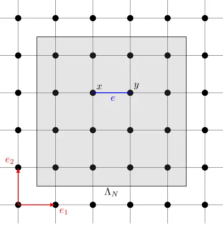
are therefore in order. The standard procedure amounts to considering finite boxes (see e.g. [6]). For a positive integer N, we denote by ΛN the finite box{0, . . . , N}d and byEN the set of edges in ΛN (see Figure 1).

e2

e1

x y

e

ΛN

Figure 1. Finite box ΛN inZ2

Thetruncated corrector ϕN

ξ defined on ΛN ×Ω is the unique solution to 

     

−∇⋆h_{A(·, ω) ξ+∇ϕ}N ξ (·, ω)

i

= 0 in ΛN, a.s.,

ϕN

ξ (·, ω) is ΛN-periodic, ϕN

ξ (0, ω) = 0 a.s.

(8)

The homogenized matrixA⋆_{, which is deterministic, is then approximated by the matrixA}⋆

N defined by

∀ξ∈Rd_{, A}⋆_N(ω)ξ= 1

|ΛN| X

x∈ΛN

A(x, ω) ξ+∇ϕNξ (x, ω)

Because of truncation, the practical approximationA⋆

N is random. In the largeN limit, the deterministic value

is attained, thanks to ergodicity. More precisely, A⋆

N(ω) converges almost surely towards A⋆ as N goes to

infinity, thanks to the ergodic theorem.

Remark 2.7. In (8), we have complemented the elliptic equation in ΛN with periodicboundary conditions.

Other choices could be made, such as imposing homogeneous Dirichlet boundary conditions: ϕN

ξ (·, ω) = 0 on ∂ΛN (see e.g. [6] for a similar discussion in the case of continuous PDEs). In the numerical experiments of

Section 4, we only use periodic boundary conditions, following (8).

In practice, we work on a finite box ΛN, on which the apparent homogenized matrix A⋆N is random. It is

therefore natural to introduce M i.i.d. realizations of the random field A(x, ω) and solve (8)–(9) for each of them, thereby obtaining i.i.d. realizations A⋆,m_N (ω), 1≤m≤M. We next introduce the empirical mean

A⋆N,M(ω) =

1

M M X

m=1

A⋆,m_N (ω) (10)

which is, according to the law of large numbers, a converging approximation ofE_[A⋆_{N]. We have that}

A⋆N,M(ω)−−−−→ M→∞

E_[A⋆_{N] a.s.}

In addition, for any entry 1≤i, j≤dof the matrix, we have that, with a probability of 95 %,

A⋆N,M(ω)

ij−

E

h

(A⋆N)ij i

≤1.96 s

V_{ar (A}⋆_N)

ij

M .

The error when approximatingA⋆ _byA⋆

N,M can be written as the sum of two contributions,

A⋆−A⋆N,M =

A⋆−E_[A⋆_N]

+E_[A⋆_N]−A⋆_N,M

. (11)

The second term in the right-hand side of (11) is the statistical error. The first term is thesystematic error, due to the fact that, for any finiteN,E_[A⋆_N]6=A⋆_{. The dominated convergence theorem ensures that this error}

vanishes asN → ∞. Many studies have been recently devoted to proving sharp estimates on the rate of this convergence, following the seminal works [6,20]. In [11, Theorem 2], the authors show (for any dimensiond≥2) that the systematic error is of orderN−d_lnd

(N) when using periodic boundary conditions (namely, solving (8)), and that V_ar(A⋆_{N) scales asN}−d_{. Likewise, in the case ofcontinuousPDEs, whend}≥3, optimal estimates on

V_ar(A⋆_{N) have been established in [17, Theorem 1.3 and Proposition 1.4].}

Remark 2.8. The estimatorA⋆N,M only agrees withE[A⋆N] in the limit of an asymptotically large numberM

of realizations. Note that variance reduction approaches have been introduced in this context (see e.g. [4, 5, 8], and [15] for the extension to a nonlinear setting) to obtain approximations ofE_[A⋆_{N] in a more efficient manner}

than by usingA⋆N,M.

In the sequel, we will identify the parameters of the microscopic probability distribution on the basis of two types of macroscopic quantities:

(1) the homogenized permeability, which is in practice approximated byA⋆N,M;

(2) the relative variance of any entry (A⋆

N(ω))ij, defined by

V_arRh_(A⋆_N)

ij i

:=

V_ar

h

(A⋆ N)ij

i

E

h

(A⋆ N)ij

which is in practice approximated by

SN,M = 1 (A⋆N,M)2ij

1

M M X

m=1

A⋆,m_N (ω)_ij−A⋆N,M

ij 2!

. (12)

2.3.

Physical problem

We describe here the physical background which inspires this work. As pointed out above, from a physical viewpoint, understanding the microscopic properties of charged porous media is of great importance. Such materials have elaborate geometries that make direct computations very challenging. To circumvent this issue, we use here the Pore Network Model (PNM), which involves a simplified model of the geometry. In the PNM model, pores are located at the vertices of the lattice Zd_{. Neighbouring pores are connected by channels,}

which allow water to flow. Each channel (x, x+ei) is endowed with its random conductanceai(x, ω)>0, the probability distribution of which is discussed below.

Experiments provide measures on the macroscopic permeability Kobs, which is modelled as a homogenized

coefficientK⋆_{. In practice, as explained in Section 2.2, the homogenized coefficient can only be approximated}

through a computation on a large box. Assuming that the conductance fieldai(x, ω) is given for any direction 1 ≤i≤dand any vertexxon the finite lattice ΛN, the PNM model consists in computing the pressure field P(x, ω) by solving the conservation equations (i.e., Darcy law) in the network. This leads to the following linear system:

∀x∈ΛN, X

y∼x

˜

a(x, y, ω) P(y, ω)−P(x, ω)= 0, (13)

where ˜a(x, y, ω) is the conductance of the non-oriented edge (x, y). Some boundary conditions need to be imposed to make this problem well-posed, they are discussed below. We next see, by definition ofai, that

X

y∼x

˜

a(x, y, ω) P(y, ω)−P(x, ω)

=

d X

i=1

ai(x, ω) P(x+ei, ω)−P(x, ω)+

d X

i=1

ai(x−ei, ω) P(x−ei, ω)−P(x, ω)

= ∇⋆_{A(·, ω)∇P(·, ω)(x), (14)}

where the matrixAis defined in terms of{ai}d_i=1by (2).

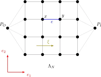
We now describe (in the two-dimensional case, for the sake of simplicity) the boundary conditions imposed on (13). They are designed to mimic experimental conditions. We first recall that the large box reads ΛN = {0, . . . , N}2_{. The pressure field is assumed to be periodic in the vertical direction, whereas a macroscopic}

gradient is imposed in the horizontal direction as follows. Imagine that all vertices with coordinates (0,·) are connected to one fixed vertex denoted by O, representing a pressure reservoir at pressure PO. Likewise, all vertices with coordinates (N,·) are connected to one fixed vertex denoted byI at pressure PI (see Figure 2). Then, the boundary conditions write

for allj∈ {0, . . . , N}, P(0, j) =PO and P(N, j) =PI.

Once (13) is solved with the above boundary conditions, the macroscopic permeability K⋆

N is defined by

KN⋆(ω) := N PO−PI

1

|ΛN| X

x∈ΛN

˜

a(x, x+e1, ω) P(x, ω)−P(x+e1, ω)

. (15)

PO PI

ξ

e2

e1

x y

e

ΛN

Figure 2. Finite lattice with boundary conditions

to (13). We introduceϕe1 such that

P(x, ω) =x·e1+ϕe1(x, ω).

In view of (13) and (14), we see thatϕe1(·, ω) is solution to

∀x∈ΛN, ∇⋆

A(·, ω)(e1+∇ϕe1(·, ω)

(x) = 0

with ϕe1((0, j), ω) =ϕe1((N, j), ω) = 0 for any j and ϕe1(·, ω) is periodic in the vertical direction. Up to the

choice of boundary conditions, we thus recognize (8) forξ=e1. We also infer from (15) that

KN⋆(ω) = N PO−PI

1

|ΛN| X

x∈ΛN

˜

a(x, x+e1, ω) P(x, ω)−P(x+e1, ω)

= −1

|ΛN| X

x∈ΛN

a1(x, ω) ϕe1(x, ω)−ϕe1(x+e1, ω)−e1·e1

= 1

|ΛN| X

x∈ΛN

a1(x, ω)eT1 e1+∇ϕe1(x, ω)

= eT1A⋆N(ω)e1,

whereA⋆

N(ω) is defined by (9), and where we have used (2) in the last line. Thus, up to the choice of boundary

conditions in the corrector problem, the formulation (13)–(15) is identical to the formulation (8)–(9).

We eventually discuss the choice of the probability distribution for the conductances. Based on experimental results, it is reasonable to assume the following:

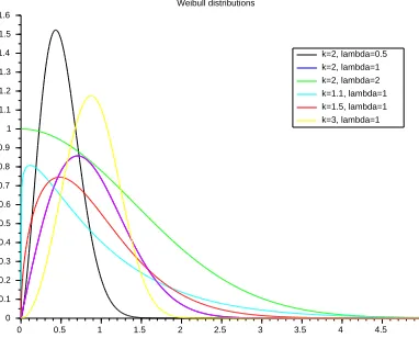
Assumption 2.9. We assume that the radiusrof the channels are i.i.d. random variables distributed according to a Weibull law of parameterθ:= (λ, k)∈(R₊⋆₎2_{, that we denote}W(λ, k). We recall that such random variables are positive, with a probability density that reads (see Figure 3)

∀r >0, f(r;k, λ) = k

λ _r

λ k−1

exp −(r/λ)k_,

corresponding to the cumulative distribution function

F(r;k, λ) =

Z r

0

Note that the radius of all channels (independently of their direction 1 ≤ i ≤ d) share the same probability distribution.

In practice, a Weibull distribution is generated as follows. Letu(ω) be a random variable uniformly distributed in [0,1]. Then

r(ω) =λh−ln(1−u(ω))i1/k

is distributed according to the Weibull law of parameter (λ, k).

Physical arguments lead to the fact that the conductanceai(x, ω) of any channel (x, x+ei) is directly related to its radiusr(x, x+ei, ω). Hereafter, we assume that

ai(x, ω) =C0r4(x, x+ei, ω) =C0λ4 h

−ln(1−ui(x, ω))i4/k, (16)

where C0 is a constant (for instance, for a Poiseuille flow, C0 = π/(8η) where η is the fluid viscosity) and

ui(x, ω) is uniformly distributed in [0,1]. For the sake of simplicity, we takeC0 = 1 in the sequel. Therefore,

we assume that

The conductances{ai(x, ω)}_x∈Zd_,1≤i≤d form an i.i.d. sequence of random variables

that are distributed according to the Weibull law of parameter (λ4, k/4). (17)

0 0.5 1 1.5 2 2.5 3 3.5 4 4.5 5 0

1

0.2 0.4 0.6 0.8 1.2 1.4 1.6

0.1 0.3 0.5 0.7 0.9 1.1 1.3 1.5

Weibull distributions

k=2, lambda=0.5 k=2, lambda=1 k=2, lambda=2 k=1.1, lambda=1 k=1.5, lambda=1 k=3, lambda=1

Figure 3. Examples of Weibull distributions.

Remark 2.10. Note that the Weibull distribution is isolated neither from 0 nor from ∞. The above model therefore does not satisfy the ellipticity condition (3). First, we show in Section 2.4.2 below that, in the one-dimensional case, the assumption (3) is not necessary, and that homogenization holds under a weaker assumption. Second, we refer to [3] for similar studies (again under assumptions weaker than (3)) in higher-dimensional cases.

Remark 2.11. The numerical tests of Section 4 are performed with the above model, and thus aim at identifying the two parametersλandk. We however note that nothing in our approach is specific to this particular model using Weibull laws. This choice is only motivated by physical reasons.

Since the conductances ai(x, ω) are all i.i.d. (for any 1≤i≤dand any x∈Zd_{), the problem is invariant}

by any rotation of angleπ/2. The homogenized matrixA⋆is therefore proportional to the identity matrix Idd,

and reads

whereK⋆_{∈(0,∞) is the homogenized permeability. We can also write that}

K⋆_=e

1·A⋆e1.

In practice, we only have access toA⋆

N(ω), which is a symmetric matrix (but is a priori not proportionnal to

the identity matrix). All directions are statistically identical, hence we only focus in the sequel on

KN⋆(ω) :=e1·A⋆N(ω)e1. (18)

2.4.

The one dimensional case

The purpose of this section is two-fold. First, we recall explicit formulas for the homogenized quantities in terms of the microscopic fieldA(x, ω). We derive these formulas assuming that (3) holds. Second, we show that we can relax Assumption (3) and still state a homogenization result.

2.4.1. Explicit formulas in the elliptic case (3)

In the one-dimensional case, the problem (8)–(9) can be analytically solved. We have

A⋆N(ω) =

1

N X

x∈ΛN

1

A(x, ω)

!−1

for almost allω. (19)

Likewise, the problem (5)–(6) can also be solved, yielding the formula

A⋆₌

E

1

A(x,·)

−1

, (20)

which can be evaluated at anyx∈Z_{due to the stationarity ofA.}

We note that, as soon asA(x, ω)>0 a.s. for any x∈Z_{and A}−1_(x,·)∈L1_{(Ω) (this latter condition being}

independent ofx), formulas (19) and (20) are well-defined. The aim of the next section is to recall that, in the one-dimensional case, these assumptions are enough for homogenization to hold.

2.4.2. Relaxing Assumption (3)

In this section, we show that the following assumption is enough for homogenization to hold:

Assumption 2.12. We assume that the coefficientA is almost surely positive and finite and satisfies

A−1_(x,·)∈L1_{(Ω). (21)}

Of course, by stationarity, if (21) is satisfied for somex∈Z_{, then it is satisfied for allx∈}Z_.

Theorem 2.13. LetDbe a bounded domain ofR_,f ∈C0_{(D)andAbe a random stationary scalar field (defined} on Z×Ω) that satisfies (21). Letuε∈ℓ2_{(εZ;R)be the unique solution to}

∇⋆ ε

A(x/ε, ω)∇εuε(x, ω)=f(x) inD ∩εZ_{, uε(x, ω) = 0in(}R\ D)∩εZ_{, (22)}

and letu⋆_∈H1

0(D)be the unique solution to the (continuous) boundary value problem

−A⋆_(u⋆₎′′ _{=f inD, (23)}

whereA⋆ _{is defined by (20).}

Then, when ε→0,uε(·, ω)converges to the homogenized solutionu⋆_{, in the sense that}

ε X

x∈D∩εZ

|uε(x, ω)−u⋆(x)|2−−−→

Note that (22) is almost surely well-posed. Indeed, sinceAis stationary and 0< A(0, ω)<∞almost surely, we have that, almost surely, 0< A(x, ω)<∞for anyx∈Z_{. For thoseω, problem (22) is well-posed. Likewise,}

sinceA is almost surely finite (resp. A−1_(0,·)∈L1_{(Ω)), we have thatA}⋆ _{<∞(resp. A}⋆_{>0) and hence (23)}

is well-posed.

Proof. The proof proceeds by truncation of the coefficientAin the neighbourhood of 0 and +∞. For the sake of simplicity, we take D= (0,1). For any m∈N⋆_{, we introduce the coefficientAmdefined on}Z_{×Ω by}

Am(x, ω) :=

      

1

m if 0< A(x, ω)<

1

m, A(x, ω) if 1

m ≤A(x, ω)≤m, m if A(x, ω)> m.

We set

A⋆m=

E

1

Am(0,·)

−1

.

For almost allω (i.e. those such thatA(0, ω)>0), we have

lim

m→∞

1

Am(0, ω) = 1

A(0, ω),

∀m∈N⋆_{, 0<} 1

Am(0, ω) ≤1 + 1

A(0, ω),

where the right-hand side of the above second line belongs to L1_{(Ω), in view of the assumption (21). Therefore,}

the dominated convergence theorem implies that

lim

m→∞A ⋆

m=A⋆. (25)

Letum

ε ∈ℓ2(εZ;R) be the unique solution to

∇⋆ ε

Am(x/ε, ω)∇εumε(x, ω)

=f(x) in (0,1)∩εZ_{, uε}m_{(x, ω) = 0 in (}R\(0,1))∩εZ_{, (26)}

and letu⋆

m∈H10(0,1) be the unique solution to the (continuous) boundary value problem

−A⋆ m(u⋆m)′

′

=f in (0,1).

We write

kuε(·, ω)−u⋆kℓ2

ε ≤ kuε(·, ω)−u

m ε(·, ω)kℓ2

ε+ku

m

ε(·, ω)−u⋆mkℓ2

ε+ku

⋆

m−u⋆kℓ2

ε (27)

where, for any functionv,

kvkℓ2

ε :=

s

ε X

x∈(0,1)∩εZ v2_(x).

We successively study the three terms of the right-hand side of (27). First, we have

lim

ε→0ku

⋆

m−u⋆kℓ2

ε =ku

⋆

m−u⋆kL2 (0,1),

and the convergence (25) implies that

lim

m→∞ε→lim0ku

⋆

m−u⋆kℓ2

Second, the coefficient Am satisfies the ellipticity condition (3), so we infer from Theorem 2.5 that, for any

m∈N⋆_,

lim

ε→0ku

m

ε (·, ω)−u⋆mkℓ2

ε = 0 a.s. (29)

We eventually turn to the first term of the right-hand side of (27). Let

Fε(x) =ε X y∈(0,x]∩εZ

f(y),

which satisfies, for any x, |Fε(x)| ≤ kfkL∞. Integrating once the equations (22) and (26), we can show that

there exist two random variablesCε(ω) andCm

ε (ω), independent ofx, such that

Amx ε, ω

∇εumε(x, ω) = −Fε(x) +Cεm(ω), (30)

Ax ε, ω

∇εuε(x, ω) = −Fε(x) +Cε(ω). (31)

Using the boundary conditions onum

ε anduε, we get

Cε(ω) =Nε(ω)

Dε(ω)

and Cεm(ω) = Nm

ε (ω) Dm

ε (ω)

where

Dε(ω) = ε X

x∈(0,1)∩εZ Ax

ε, ω −1

, Nε(ω) =ε X

x∈(0,1)∩εZ Ax

ε, ω −1

Fε(x),

Dm

ε(ω) = ε X

x∈(0,1)∩εZ Amx

ε, ω −1

, Nm ε (ω) =ε

X

x∈(0,1)∩εZ Amx

ε, ω −1

Fε(x).

All these quantities are well-defined for almost all ω. We claim that

lim

m→∞lim sup_ε→0 |Cε(ω)−C m

ε (ω)|= 0 a.s. (32)

To prove this claim, we start by writing that

Cε(ω)−Cεm(ω) =

Nε(ω)− Nεm(ω) Dε(ω)

+ N

m ε (ω) Dm

ε (ω)Dε(ω)

(Dεm(ω)− Dε(ω)). (33)

Introduce

bm(x, ω) =

_Am(1_{x, ω)}−_{A(x, ω}1 ₎

and Bεm(ω) =ε X

x∈(0,1)∩εZ bmx

ε, ω

.

For anym∈N⋆_{, we get}

|Nm

ε (ω)− Nε(ω)| ≤ kfkL∞ ε X

x∈(0,1)∩εZ bmx

ε, ω

=kfkL∞ Bm

ε(ω), (34)

|Dm

ε(ω)− Dε(ω)| ≤ ε X

x∈(0,1)∩εZ bmx

ε, ω

=Bm

ε (ω), (35)

|Nm

ε (ω)| ≤ kfkL∞ Dm

Using the ergodic theorem for the stationary functionsA−1_,A−1

m andbm, we have that, for anym∈N⋆, almost

surely,

lim

ε→0Dε(ω) =

1

A⋆, _ε→lim₀D m ε (ω) =

1

A⋆ m

, lim

ε→0B

m

ε(ω) =Bm⋆ :=E

1

Am(0,·)− 1

A(0,·)

. (37) We introduce

Ωconv=

ω∈Ω; lim

ε→0Dε(ω) =

1

A⋆ and, for allm∈N ⋆_{, lim}

ε→0D

m ε (ω) =

1

A⋆ m

, lim

ε→0B

m

ε (ω) =Bm⋆

and we deduce thatP_{(Ωconv) = 1.}

Letω∈Ωconv. In view of (37), we know that there existsεm0 (ω) such that, for anyε < εm0 (ω), we have

1

2A⋆ ≤ Dε(ω),

1 2A⋆

m ≤ Dm

ε(ω)≤

3 2A⋆

m

. (38)

We thus infer from (33), (38), (34), (36) and (35) that, for any ω∈Ωconv, any m∈N⋆ and any ε < εm0(ω), we

have

|Cε(ω)−Cεm(ω)| ≤ 2A⋆|Nε(ω)− Nεm(ω)|+ 4A⋆A⋆m|Nεm(ω)| |Dεm(ω)− Dε(ω)| ≤ 2A⋆ _kfk

L∞ Bm

ε (ω) + 4A⋆A⋆mkfkL∞ Dm

ε (ω)Bmε (ω) ≤ 2A⋆ kfkL∞ Bm

ε (ω) + 6A⋆ kfkL∞ Bm

ε(ω). (39)

Hence, for anyω∈Ωconvand any m∈N⋆, we have

lim sup

ε→0

|Cε(ω)−Cεm(ω)| ≤8A⋆ kfkL∞ B⋆

m.

The dominated convergence theorem implies that lim

m→∞B ⋆

m= 0, hence, for anyω∈Ωconv, we have

lim

m→∞lim sup_ε→0 |Cε(ω)−C m

ε (ω)|= 0.

SinceP_{(Ωconv) = 1, we have proved the claim (32).}

We now proceed and deduce from (30) and (31) that

umε (z, ω) = ε X

x∈(0,z)∩εZ Amx

ε, ω −1

(Cεm(ω)−Fε(x)),

uε(z, ω) = ε X x∈(0,z)∩εZ

Ax ε, ω

−1

(Cε(ω)−Fε(x)),

hence

|umε(z, ω)−uε(z, ω)| ≤ |Cεm(ω)−Cε(ω)| Dεm(ω) + (|Cε(ω)|+kfkL∞) Bm

ε (ω).

Using that |Cε(ω)| ≤ kfkL∞, we deduce that

kumε (·, ω)−uε(·, ω)kℓ2

ε≤ |C

m

ε (ω)−Cε(ω)| Dεm(ω) + 2kfkL∞ Bm

ε(ω).

For anyω∈Ωconv, anym∈N⋆ and any ε < εm0 (ω), using (39) and (38), we obtain that

kum

ε(·, ω)−uε(·, ω)kℓ2

ε≤8A

⋆ _kfk

L∞ Bm

ε (ω)

3 2A⋆

m

+ 2kfkL∞ Bm

hence, for anyω∈Ωconv and anym∈N⋆,

lim sup

ε→0

kumε(·, ω)−uε(·, ω)kℓ2

ε ≤8A

⋆ _kfk

L∞ Bm

⋆

3 2A⋆

m

+ 2kfkL∞ Bm

⋆ ,

and thus, almost surely,

lim

m→∞lim sup_ε→0 ku m

ε (·, ω)−uε(·, ω)kℓ2

ε = 0. (40)

Collecting (27), (28), (29) and (40), we obtain that

lim sup

ε→0

kuε(·, ω)−u⋆kℓ2

ε= 0 a.s.,

which is the convergence (24).

2.4.3. The case of Weibull laws

Following Section 2.3, assume that the conductances are given by (17), i.e. are distributed according to the Weibull law of parameter (λ4_{, k/4). For any k > 0, Assumption (3) is not satisfied. However, whenk > 4,}

Assumption (21) is satisfied: in view of Theorem 2.13, homogenization holds and the homogenized coefficient is given by

A⋆= λ

4

Γ(1−4/k), (41)

where Γ is the Euler Gamma function defined for anyz >0 by

Γ(z) =

Z ∞

0

tz−1 exp(−t)dt. (42)

The variance ofA⋆

N is finite if and only ifk >8. In the sequel, we work in the rangek >8.

3.

A parameter fitting problem

We now describe the problem we consider, first in the general case (Section 3.1), next in the one-dimensional case (Section 3.2). In that latter section, we also motivate our choice of macroscopic quantities from which we fit the parameters of the Weibull law.

3.1.

General case

We assume that we are given two observed quantities, the first coefficient of the macroscopic permeability matrix (see (18))

KN⋆,obs(ω) =e1·A⋆,Nobs(ω)e1

and its relative varianceSobs

N for some parameterθobs= (λobs, kobs) of the Weibull law. Note that the relative

variance crucially depends on the sizeNd _{of the finite box on which it is measured (in contrast to the apparent}

permeability, which converges to a finite value when N → ∞). We assume here that we know this size. In practice, these three quantities, N, K_N⋆,obs and Sobs

N , can be obtained by physical experiments. We therefore

assume that there existsθobs andN such that

E_[KN⋆_{(·, θobs)] =K}⋆,obs

N , VarR[K ⋆

N(·, θobs)] =SNobs, (43)

where, we recall,

V_arR[KN⋆_{(·, θobs)] =} Var[K

⋆

N(·, θobs)]

(E_[K⋆

N(·, θobs)])2

Given N, K_N⋆,obs and Sobs

N , our aim is to recover (an approximation of)θobs. To that aim, we consider the

function FN,M :       

(R⋆₊₎2 _→ R₊

θ 7→ K

⋆ N,M(θ) K_N⋆,obs −1

!2

+

SN,M(θ)

Sobs

N

−1

2 ₍₄₄₎

which penalizes the sum of the (relative) errors between

• on the one hand, K⋆N,M(θ) (which is an empirical estimator of E[KN⋆(·, θ)] when M is large, see (10)

and (18)) and K_N⋆,obs

• and, on the other hand, SN,M(θ) (which is an empirical estimator of the relative variance ofK⋆ N(ω, θ)

whenM is large, see (12) and (18)) andSobs

N .

Of course, different weights could be assigned to the error on the permeability and the error on its relative variance. We eventually cast our parameter fitting problem in the form of the optimization problem

inf

θ=(λ,k)∈(0,∞)×KFN,M(θ),

whereK ⊂(0,∞) is the admissible set of parametersksuch that homogenization holds (even if Assumption (3) is not satisfied for anyk >0) and the variance ofK⋆

N is also well-defined. In the one-dimensional case we focus

on in this article,K= (8,∞).

Note that FN,M(θ) is random, as it depends on the realizations used to evaluate K⋆N,M(θ) and SN,M(θ)

(see (10) and (12)). For anyθ, in the limit whenM → ∞,FN,M(θ) converges almost surely to the deterministic limit

FN(θ) = E[K

⋆ N(·, θ)] K_N⋆,obs −1

!2

+

_V

arR[K⋆ N(·, θ)] Sobs

N

−1

2

.

Under Assumption (43), we have

FN(θ) =

_E

[K⋆ N(·, θ)]

E_[K⋆

N(·, θobs)] −1

2

+

_V

arR[K⋆ N(·, θ)]

V_arR[K⋆

N(·, θobs)] −1

2

.

3.2.

The one-dimensional case

Recall that, in that case,K⋆

N =A⋆N (see (18)).

3.2.1. Theoretical result

We first identify the limit when N→ ∞ofFN, which we recall reads

FN(θ) =

_E

[A⋆ N(·, θ)]

E_[A⋆

N(·, θobs)] −1

2

+

_V

arR[A⋆ N(·, θ)]

V_arR[A⋆

N(·, θobs)] −1

2

. (45)

Obviously, the first term above converges to

A⋆_(θ) A⋆_(θ

obs) −1

2

,

with, following (41),

A⋆₌ λ4

For the second term of (45), it is clear that V_arR[A⋆

N(·, θ)] vanishes in the limit N → ∞, since A⋆N(·, θ)

converges almost surely to a deterministic limit. Furthermore, equation (19) implies that

V_ar[A⋆_{N] =} (A

⋆₎4

N Var

1

A(0,·)

+o

1

N

. (46)

The conductances are distributed according to a Weibull law (see (17)), therefore

V_ar[A⋆_{N] =} λ

16

NΓ(1−4/k)4

Γ(1−8/k)

λ8 −

Γ(1−4/k)2

λ8

+o

1

N

,

hence the relative variance reads

V_arR[A⋆_{N] =} 1

N

Γ(1−8/k) Γ(1−4/k)2 −1

+o

1

N

, (47)

which implies that

lim

N→∞

V_arR[A⋆_N(·, θ)]

V_arR[A⋆

N(·, θobs)]

=

Γ(1−8/k) Γ(1−4/k)2 −1 Γ(1−8/kobs) Γ(1−4/kobs)2 −1

.

In the one-dimensional case, we are thus able to identify the limit asN → ∞ofFN(θ), which reads

F∞1D(θ) := lim

N→∞FN(θ) =

λ4

λ4 obs

Γ(1−4/kobs)

Γ(1−4/k) −1

2

+

 

Γ(1−8/k) Γ(1−4/k)2 −1 Γ(1−8/kobs) Γ(1−4/kobs)2 −1

−1

  2

. (48)

Obviously, this function is minimal (and vanishes) whenθ=θobs. It turns out that this minimizer is the unique

minimizer, as shown below.

Lemma 3.1. The function F1D

∞ defined by (48)has a unique minimizer, which isθobs.

Homogenization is an averaging process, which filters out many features of the microscopic coefficient A. These features cannot be recovered from the knowledge of macroscopic quantities. The above lemma shows (in the one-dimensional case) that, if one assumes a given form for the probability distribution of A (here, a Weibull distribution), then one is able to recover the two parameters of that law on the basis of two macroscopic quantities, the permeability and its relative variance.

It is also obvious from (41) that knowing the macroscopic permeability is not enough to uniquely determine the two parametersλ and kof the Weibull law. Additional information is needed. Our choice of considering the relative variance of the permeability is motivated by the following observation. This quantity, in the one-dimensional case, only depends (at first order in N) on k and does not depend onλ, as can be seen on (47). Knowing this quantity is therefore very useful to estimate the parameterk. Oncekhas been identified, knowing the macroscopic permeability yields, using (41), an estimation of the parameterλ.

Of course, it is likely that the knowledge of quantities of interest alternate to the relative variance of the permeability may also prove useful to determine the unknown parameters. Note also that such alternate relevant quantities should be “different enough” from the homogenized permeability to indeed bring new information. We do not pursue in that direction.

We plot on Figure 4 the functionθ7→F1D

∞ (θ) forλobs= 1 andkobs= 15. We observe that the function is not

degenerated at its minimum, in the sense that its Hessian matrix at θobs is positive definite, with eigenvalues

equal to 16 and 0.04. We thus expect that a standard algorithm (such as the Newton algorithm) will be able to converge to the minimizer ofF1D

Figure 4. Plot ofθ7→F1D

∞ (θ) forλobs = 1 andkobs = 15. The bottom plot is a zoom of the

top plot around the minimizer.

Proof of Lemma 3.1. The proof consists of three steps: in Step 1, we recall (and prove for the sake of complete-ness) that ln Γ is a convex function. In Step 2, we prove that the function

ζ:k7→ Γ(1−8/k)

is monotone (hence injective). We conclude in Step 3.

Step 1.From (42), we compute that, for anyz >0,

Γ′_{(z) =}

Z ∞

0

(lnt)tz−1 _exp(−t)dt,

Γ′′_{(z) =}

Z ∞

0

(lnt)2tz−1exp(−t)dt,

therefore Γ′′_{(z)>0 and Γ is positive and convex on (0,∞). In addition, we have}

(ln Γ)′′(z) =Γ(z)Γ

′′_(z)−(Γ′_(z))2

Γ2_(z)

which is positive, in view of the Cauchy-Schwartz inequality:

(Γ′_(z))2₌

Z ∞

0

(lnt)ptz−1 _exp(−t) p_tz−1_exp(−t)dt 2

<Γ′′_(z)Γ(z).

Therefore, ln Γ is a strictly convex function.

Step 2.We define the function

ζ:k7→ Γ(1−8/k)

Γ(1−4/k)2,

the derivative of which reads

ζ′(k) = Γ(1−8/k) Γ(1−4/k)2

8

k2

Γ′_(1−8/k)

Γ(1−8/k) − 8

k2

Γ′_(1−4/k)

Γ(1−4/k)

.

For any k >0, we have that 1−8/k <1−4/k. As a consequence of ln Γ being strictly convex, we have that its derivative is increasing, therefore

Γ′_(1−8/k)

Γ(1−8/k) <

Γ′_(1−4/k)

Γ(1−4/k). We can now conclude thatζ′_{(k)<0, henceζ is decreasing.}

Step 3.By definition ofζ, we have that

F1D

∞ (θ) =

λ4

λ4 obs

Γ(1−4/kobs)

Γ(1−4/k) −1

2

+

ζ(k)−1

ζ(kobs)−1 −1

2

.

We obviously have that θobs is a minimizer of F∞1D, with F∞1D(θobs) = 0. Conversely, let θ be a minimizer of

F1D

∞ . We thus haveF∞1D(θ) = 0, which implies thatζ(k) =ζ(kobs). The functionζbeing monotone, this implies

thatk=kobs. Since the first term inF∞1D(θ) also vanishes, we obtain thatλ=λobsas well. This concludes the

proof.

3.2.2. Practical situation

In the general (i.e. multi-dimensional) case, we have introduced in (44) the function FN,M that we wish to minimize. Turning next to the one-dimensional case, we have theoretically identified its limit when M → ∞

andN → ∞. In practice, we cannot take any of these limits, and have thus to work withFN,M defined by

FN,M(θ) = K

⋆ N,M(θ) KN⋆,obs

−1

!2

+

SN,M(θ)

Sobs

N −1

2

In view of (46), we see that, whenM → ∞and nextN → ∞, the relative varianceSN,M(θ) is close to

SN,M(θ)≈(A ⋆₎2

N Var

1

A(0,·)

= E[W

−8_{]− E[W}−4_]2

N (E_[W−4_])2 =

E_[W−8_]

N (E_[W−4_])2−

1

N,

whereW is a random variable distributed according to the Weibull lawW(1, k). Likewise,

K⋆N,M(θ)≈A⋆= λ4

E_[W−4_].

Let{ui(ω)}N_i=1 be a sequence of i.i.d. random variables uniformly distributed in [0,1]. We define

wi(k, ω) := (−ln(1−ui(ω)))−1/k_{, (49)}

so that{1/wi(k, ω)}N_i=1 are i.i.d. random variables distributed according toW(1, k). In the sequel, we approx-imate the function to minimize by

e

FN1D(θ, ω) = 

 λ4

K_N⋆,obs "

1

N N X

i=1

wi4(k, ω) #−1

−1

  2

+

  _S1obs

N   

PN

i=1w8i(k, ω)

PN

i=1wi4(k, ω) 2−

1

N   −1

   2

. (50)

This function is consistent in the sense that it almost surely converges, whenN→ ∞, to the exact function (48). On the other hand,Fe1D

N (θ, ω) is random, and thus somewhat mimics the difficulties that one would encounter

in the multi-dimensional case when working withFN,M(θ).

4.

Numerical results

We briefly explain in Section 4.1 how in practice we minimize the function (50), before turning in Section 4.2 to our numerical results. As pointed out in the introduction, we only consider here the one-dimensional case, and postpone the study of two-dimensional examples to the future work [16].

4.1.

Optimization algorithm

We provide in Appendix A expressions for the first and second derivatives of the functionFe1D

N (θ, ω) defined

by (50) with respect toθ= (λ, k). We are thus in position to use the Newton algorithm, and compute a sequence

θj according to

θj+1=θj−µj h

HFeN1D

(θj)i

−1

∇FeN1D(θj), (51)

where HFe1D

N

∈ R2×2 _{is the Hessian matrix of Fe}1D

N and ∇FeN1D ∈ R2 is the gradient of FeN1D (for the sake

of simplicity, we keep implicit the dependence with respect to ω). In turn, µj >0 is the step-size by which we move. To choose µj, we have used a line-search algorithm (along the descent direction prescribed by the Newton algorithm) using Goldstein (respectively Armijo) rule to increase (respectively decrease) the step-size.

We note that the function θ 7→ F1D

∞ (θ) is not convex. It is possible to find some θ such that the Hessian

matrixH F1D

∞

(θ) is not positive definite, but rather has (at least) one negative eigenvalue. We thus cannot expect the function θ 7→Fe1D

N (θ) to be convex (even for large values of N), and the Newton algorithm to be

globally convergent. We are therefore careful to start the Newton iterations from an initial guessθ0 (given by

physical experiments) that we hope to be close enough to the minimizer ofFe1D

4.2.

Numerical results

In all what follows, we setN = 105_.

4.2.1. Robustness of the algorithm with respect to the initial guess

Our first numerical test is a simple one, to check whether the Newton algorithm (51) is indeed able to minimize the function θ7→Fe1D

N (θ, ω). We pick once for all one realization of the i.i.d. random variables {ui(ω)}1≤i≤N

(which, we recall, are uniformly distributed in [0,1]). We then build {wi(k, ω)}_1≤i≤N according to (49) and consider the functionθ7→Fe1D

N (θ, ω) defined by (50), where the observed quantities are defined by

K_N⋆,obs=λ4obs " 1 N N X i=1

wi4(kobs, ω) #−1

, SNobs= PN

i=1wi8(kobs, ω)

PN

i=1w4i(kobs, ω) 2 −

1

N,

withλobs= 1 andkobs= 15. The functionθ7→FeN1D(θ, ω) obviously vanishes atθobs= (λobs, kobs).

We run the Newton algorithm (51) starting from several initial guessesθ0, and check that it indeed always

converges to θobs in a limited number of iterations. We also observe that, for some initial guesses, using an

adaptive step-size µj as in (51) is critical: in contrast, if one uses the step-sizeµj = 1, then the algorithm may not converge, or converges after a much larger number of iterations.

4.2.2. Robustness with respect to statistical noise

For our second test, we proceed as follows. We first setθref= (λref, kref) = (1,15) and pick one realization of

the i.i.d. random variables {ui(ω)}_1≤i≤N (which, we recall, are uniformly distributed in [0,1]). We then build

{wi(kref, ω)}1≤i≤N according to (49) and define the macroscopic observed quantities as

K_N⋆,obs=λ4ref " 1 N N X i=1

w4i(kref, ω) #−1

, SNobs= PN

i=1w8i(kref, ω)

PN

i=1wi4(kref, ω) 2−

1

N. (52)

We now fix the initial guess θ0 = (1.1,16.5) (10% off the reference value θref) and set M = 500. For any

1≤m≤M, we perform the following procedure:

• we draw a realization ofNi.i.d. random variables{ui(ωm)}_1≤i≤N which is independent of the realization

{ui(ωm′)}

1≤i≤N for any m

′ _{6= m, and independent of the realization{ui(ω)}}

1≤i≤N used to compute K_N⋆,obs andSobs

N in (52);

• using{ui(ωm)}_1≤i≤N, we buildwi(k, ωm) according to (49) and we consider the functionθ7→FeN1D(θ, ωm)

defined by (50), i.e.

e

FN1D(θ, ωm) = 

 λ4

K_N⋆,obs " 1 N N X i=1

w4i(k, ωm) #−1

−1   2 +   _Sobs1

N   

PN

i=1w8i(k, ωm)

PN

i=1w4i(k, ωm) 2 −

1

N   −1

   2

.

Recall that the macroscopic observed quantities are independent ofωm.

• we run the Newton algorithm (51) to minimize the function θ7→Fe1D

N (θ, ωm). The optimal parameter

found by the algorithm depends onωmand is denotedθopt(ωm). Since the realizationωmis different

from the reference realizationω, we have in generalθopt(ωm)6=θref.

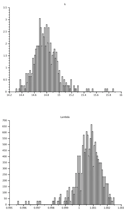
We show on Figure 5 the histogram of the optimal parameters θopt(ωm) for 1 ≤ m ≤ M. We see that

E_{(θopt)6=θref. We also observe that the width of these histograms (related to the variance ofkopt andλopt) is}

quite small.

Remark 4.1. Of course, the variance of kopt and λopt is related to N. In the limit N → ∞, the function e

F1D

N (θ, ω) almost surely converges to the deterministic limit F∞1D(θ) defined by (48), and we thus expectkopt

and λopt to almost surely converge to a deterministic limit. But this is not the regime we are interested in,

since in practice (in the two-dimensional case), we have to work with therandomfunctionFN,M.

Figure 5. Top: distribution ofkopt(ω). Bottom: distribution ofλopt(ω).

We next compare the variance of θopt with the amount of randomness introduced in the functionFeN1D(·, ω)

defined by (50). By construction,

e

FN1D(θ, ω) = K⋆

N(θ, ω) KN⋆,obs

−1

!2

+

SN(k, ω)

Sobs

N

−1

with

SN(k, ω) =

  

PN

i=1w8i(k, ω)

PN

i=1wi4(k, ω) 2 − 1 N   ,

which is an approximation of the relative variance of K⋆

N(θ, ω). We show on Figure 6 the histograms, for

1≤m≤M, ofK⋆

N(θ0, ωm) and ofSN(k0, ωm), for the initial guess parameterθ0= (1.1,16.5).

On this test-case, we compute thatV_{ar[λopt]≈7.9 10}−7 _andV_{ar[kopt]≈3.8 10}−2_{, thus}

V_{arR[λopt]≈7.9 10}−7 _and V_{arR[kopt]≈1.7 10}−4_.

On the other hand,A⋆_(θ

0)≈1.2,Var [A⋆N(θ0)]≈2.0 10−6 andVar [SN(k0)]≈4.5 10−15, thus

V_{arR [KN}⋆_(θ0)]≈1.4 10−6 _{and VarR [SN(k}

0)]≈10−3.

We thus observe that the relative variance of the optimal parameters is roughly of the same order of magnitude as the relative variance introduced in the function to minimize. Given the amount of noise present in the system, our procedure robustly identifies the optimal parameters of the microscopic distribution.

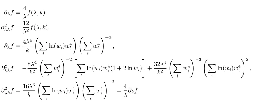
A.

Computation of the derivatives of

(50)

We introduce

f(λ, k) :=λ4 N X

i=1

w4i(k) !−1

and

g(k) :=

N X

i=1

wi8(k) ! _N

X

i=1

wi4(k) !−2

wherewi(k) is defined by (49), and recast the function (50) as

e

FN1D(θ) = N

K_N⋆,obs f(λ, k)−1 !2 + 1 Sobs N

g(k)− 1 N

−1

2

,

where we have kept implicit the dependence with respect to ω. Computing the derivatives of Fe1D

N therefore

amounts to computing those off andg.

A tedious but straightforward computation leads to the following expressions:

g′_{(k) =}8 k

X

i wi4

!−2" P

iwi8 P

iwi4 X

i

ln(wi)w4i − X

i

ln(wi)w8i #

,

g′′(k) =16

k2 X

i w4i

!−2" X

i

ln(wi)w8i(1 + 4 lnwi)− P

iw8i P

iw4i X

i

ln(wi)w4i(1 + 2 lnwi) #

−32 k2

X

i wi4

!−3

4 X

i

wi8ln(wi) !

X

i

wi4ln(wi) !

−3 X

i

wi4ln(wi) !2_P

iwi8 P

Figure 6. Top: distribution ofK⋆

N(θ0, ω). Bottom: distribution ofSN(k0, ω).

whereas

∂λf = 4

λf(λ, k),

∂λλ2 f =

12

λ2f(λ, k),

∂kf = 4λ

4

k X

i

ln(wi)wi4 !

X

i wi4

!−2

,

∂kk2 f =−

8λ4

k2 X

i w4i

!−2" X

i

ln(wi)w4i(1 + 2 lnwi) #

+32λ

4

k2 X

i w4i

!−3 X

i

ln(wi)w4i !2

,

∂2λkf =

16λ3

k X

i

ln(wi)w4i !

X

i w4i

!−2

= 4

Acknowledgements. We thank Tony Leli`evre for giving us the opportunity to work on this problem during the CEMRACS 2013 (http://smai.emath.fr/cemracs/cemracs13/), and Nicolas Champagnat, Tony Leli`evre and Anthony Nouy for the organization of this event. We are grateful to Samir B´ekri, Daniel Coelho, Claude Le Bris, Tony Leli`evre and Benjamin Rotenberg for enlightening discussions. The work of FL and WM is partially supported by ONR under Grant N00014-12-1-0383. WM gratefully acknowledges the support from Labex MMCD (Multi-Scale Modelling & Experimentation of Materials for Sustainable Construction) under contract ANR-11-LABX-0022. WM, AO and MS acknowledge financial support from NEEDSMilieux Poreux.

References

[1] A. Anantharaman, R. Costaouec, C. Le Bris, F. Legoll and F. Thomines, Introduction to numerical stochastic homogenization and the related computational challenges: some recent developments, W. Bao and Q. Du eds., Lecture Notes Series, Institute for Mathematical Sciences, National University of Singapore, volume 22, 197–272 (2011).

[2] A. Bensoussan, J.-L. Lions and G. Papanicolaou,Asymptotic analysis for periodic structures, Studies in Mathematics and its Applications, vol. 5. North-Holland Publishing Co., Amsterdam-New York, 1978.

[3] M. Biskup, Recent progress on the random conductance model,Probability Surveys,8(2011), 294–373.

[4] X. Blanc, R. Costaouec, C. Le Bris and F. Legoll, Variance reduction in stochastic homogenization: the technique of antithetic variables, in Numerical Analysis and Multiscale Computations, B. Engquist, O. Runborg and R. Tsai eds., Lect. Notes Comput. Sci. Eng., vol. 82, Springer, 47-70 (2012).

[5] X. Blanc, R. Costaouec, C. Le Bris and F. Legoll, Variance reduction in stochastic homogenization using an-tithetic variables, Markov Processes and Related Fields, 18(1) (2012), 31–66 (preliminary version available at

http://cermics.enpc.fr/∼legoll/hdr/FL24.pdf).

[6] A. Bourgeat and A. Piatnitski, Approximation of effective coefficients in stochastic homogenization,Ann. I. H. Poincar´e -PR,40(2) (2004), 153–165.

[7] D. Cioranescu and P. Donato,An introduction to homogenization, Oxford Lecture Series in Mathematics and its Appli-cations, vol. 17. Oxford University Press, New York, 1999.

[8] R. Costaouec, C. Le Bris and F. Legoll, Variance reduction in stochastic homogenization: proof of concept, using antithetic variables,Boletin Soc. Esp. Mat. Apl.,50(2010), 9–27.

[9] B. Engquist and P. E. Souganidis, Asymptotic and numerical homogenization,Acta Numerica,17(2008), 147–190. [10] I. Fatt, The network model of porous media,Trans. AIME,207(1956), 144–181.

[11] A. Gloria, S. Neukamm and F. Otto,Quantification of ergodicity in stochastic homogenization: optimal bounds via spectral gap on Glauber dynamics, Invent. Math., DOI 10.1007/s00222-014-0518-z, published online in 2014.

[12] V. V. Jikov, S. M. Kozlov, and O. A. Oleinik, Homogenization of differential operators and integral functionals, Springer-Verlag, 1994.

[13] R. K¨unnemann, The diffusion limit for reversible jump processes on Zd

with ergodic random bond conductivities,Comm. Math. Phys.,90(1) (1983), 27–68.

[14] S. M. Kozlov, Averaging of difference schemes,Math. USSR Sbornik,57(2) (1987), 351–369.

[15] F. Legoll and W. Minvielle, Variance reduction using antithetic variables for a nonlinear convex stochastic homogenization problem,Discrete and Continuous Dynamical Systems - Series S,8(1) (2015), 1–27.

[16] F. Legoll, W. Minvielle, A. Obliger and M. Simon, in preparation.

[17] J. Nolen, Normal approximation for a random elliptic equation,Probability Theory and Related Fields,159(3) (2014), 661–700. [18] J. Nolen, G.A. Pavliotis and A.M. Stuart, Multiscale modelling and inverse problems, in Numerical Analysis of Multiscale Problems, I.G. Graham, T. Hou, O. Lakkis and R. Scheichl eds., Lect. Notes Comput. Sci. Eng., vol. 83, Springer, 1-34 (2012). [19] G.C. Papanicolaou and S.R.S. Varadhan, Boundary value problems with rapidly oscillating random coefficients, inProc. Colloq. on Random Fields: Rigorous Results in Statistical Mechanics and Quantum Field Theory, J. Fritz, J.L. Lebaritz and D. Szasz, eds, Colloquia Mathematica Societ. Janos Bolyai, Vol. 10, North-Holland, Amsterdam, 1981, pp. 835–873.