N. Champagnat, T. Leli`evre, A. Nouy, Editors
EMULATORS FOR STOCHASTIC SIMULATION CODES
Vincent Moutoussamy
1,2, Simon Nanty
3,4and Benoˆıt Pauwels
2,5Abstract. Numerical simulation codes are very common tools to study complex phenomena, but they are often time-consuming and considered asblack boxes. For some statistical studies (e.g. asset management, sensitivity analysis) or optimization problems (e.g. tuning of a molecular model), a high number of runs of such codes is needed. Therefore it is more convenient to build a fast-running approximation – or metamodel – of this code based on a design of experiments. The topic of this paper is the definition of metamodels forstochasticcodes. Contrary to deterministic codes, stochastic codes can give different results when they are called several times with the same input. In this paper, two approaches are proposed to build a metamodel of the probability density function of a stochastic code output. The first one is based onkernel regression and the second one consists in decomposing the output density on a basis of well-chosen probability density functions, with a metamodel linking the coefficients and the input parameters. For the second approach, two types of decomposition are proposed, but no metamodel has been designed for the coefficients yet. This is a topic of future research. These methods are applied to two analytical models and three industrial cases.
R´esum´e. Les codes de simulation num´erique sont couramment utilis´es pour ´etudier des ph´enom`enes complexes. Ils sont cependant souvent coˆuteux en temps de calcul. Pour certaines ´etudes statistiques (e.g. gestion d’actifs, analyse de sensibilit´e) ou probl`emes d’optimisation (e.g. r´eglage des param`etres d’un mod`ele mol´eculaire), un grand nombre d’appels `a de tels codes est n´ecessaire. Il est alors plus appropri´e d’´elaborer une approximation – ou m´etamod`ele – peu coˆuteuse en temps de calcul `a partir d’un plan d’exp´erience. Le sujet de cet article est la d´efinition de m´etamod`eles pour des codes stochas-tiques. Contrairement aux codesd´eterministes, les codes stochastiques peuvent renvoyer des r´esultats diff´erents lorsqu’ils sont appel´es plusieurs fois avec le mˆeme jeu de param`etres. Dans cet article deux approches sont propos´ees pour la construction d’un m´etamod`ele de la densit´e de probabilit´e de la sortie d’un code stochastique. La premi`ere repose sur la r´egression `a noyau et la seconde consiste `
a d´ecomposer la densit´e de la sortie du code dans une base de densit´es de probabilit´e bien choisies, avec un m´etamod`ele exprimant les coefficients en fonction des param`etres d’entr´ee. Pour la seconde approche, deux types de d´ecomposition sont propos´es, mais aucun m´etamod`ele n’a encore ´et´e ´elabor´e pour les coefficients: c’est un sujet de recherches futures. Ces m´ethodes sont appliqu´ees `a deux cas analytiques et trois cas industriels.
1 EDF R&D, MRI, Chatou, France; e-mail:
2 Universit´e Paul Sabatier, Toulouse, France
3 CEA, DEN, DER, F-13108 Saint-Paul-Lez-Durance, France; e-mail:[email protected] 4 Universit´e Joseph Fourier, Grenoble, France
5 IFPEN, DTIMA, Rueil-Malmaison, France; e-mail:[email protected]
c
EDP Sciences, SMAI 2015
Introduction
Numerical simulation codes are very common tools to study complex phenomena. However these computer codes can be intricate and time-consuming: a single run may take from a few hours to a few days. Therefore,
when carrying out statistical studies (e.g. sensitivity analysis, reliability methods) or optimization processes
(e.g. tuning of a molecular model), it is more convenient to build an approximation – or metamodel – of the
computer code. Since this metamodel is supposed to take less time to run than the actual computer code, it
is substituted for the numerical code. A numerical code is said deterministic if it gives the same output each
time it is called with a given set of input parameters. For this case, the design of metamodels has already been widely studied. The present work deals with the formulation of a metamodel for a numerical code which
is not deterministic, but stochastic. Two types of numerical codes can be covered by this framework. First,
the code under consideration may be intrinsically stochastic: if the code is called with the same input several
times, the output may differ. Thus, the output conditionally to the input is itself a random variable. Second, the computer code may be deterministic with complex inputs. For example, these inputs may be functions or
spatiotemporal fields. These complex inputs are not treated explicitly and are calleduncontrollable parameters,
while the other parameters are considered ascontrollable parameters. When the code is run several times with
the same set of controllable parameters, the uncontrollable parameters may change, and thus different output values may be obtained: the output is a random variable conditionally to the controllable parameters.
Two types of approaches can be found in the literature for stochastic code metamodeling. In the first one,
strong hypotheses are made on the shape of the conditional distribution of the output. In [24] the authors
consider that the output is normally distributed and estimate its mean and variance, in [23] the authors assume
that the distribution of the output of the code is a mixture of normal distributions and estimate its mean.
In the second approach, the mean and variance of the output are fitted jointly. In [13,31] the authors use
joint generalized linear models and joint generalized additive models respectively to fit these quantities. Joint
metamodels based on Gaussian processes have been developed in [3,17]. As we can observe, so far in the
literature the metamodels proposed only provide an estimate for one or two of the output distribution moments, sometimes under strong hypotheses on the distribution of the output.
Our approach does not require such a priori hypotheses. Furthermore we study the whole distribution of the output, allowing to derive estimations for the mean, variance and other moments, and quantiles as well. The metamodeling is not carried out on the stochastic computer code under consideration itself, but rather on
the codeGthat has same input and that returns the probability density function of the computer code output
rather than just a single random value:
G:X ⊂Rd→ F
x7→G(x,•),
whereF is the space of probability density functions with support in an intervalI ofR:
F =
f :I→R+:
Z
I
f = 1
.
LetXN ={(xi, fi) :i= 1, . . . , N} ⊂(X× F)N be atraining set(N∈N\ {0}): we suppose that we have access
to the probability density functions fi of the outputs associated withN given sets of input parametersxi,i.e.
fi=G(xi,•) (i= 1, . . . , N).
In practice, for a given i in {1, . . . , N}, the output of a stochastic computer code is not a probability density
function fi. We only have access to a finite sample of output values yi1, . . . , yiM which can be written as a
vector
−20 −10 0 10 20
0.0
0.1
0.2
0.3
0.4
x
f
mean = −10, sd = 3 mean = 0, sd = 1 mean = 5, sd = 10
Figure 1. Probability density function given by the numerical codeGfor different values of
the input parameters.
derive each probability density functionfi thanks to kernel density estimation. In this non-parametric method
developed by Rosenblatt [25] and Parzen [21], the estimator of the probability density functionfi,i= 1, . . . , N
at a pointy inI is defined as follows:
ˆ
fi(y) = 1
M
M X
j=1
KH(yij−y),
where H ∈Ris the bandwidth andKH is the kernel. Letx0∈X be a new set of input parameters, we want
to estimate the probability density function f0 of the corresponding output:
f0=G(x0,•) :I⊂R→R+
t7→f0(t) =G(x0, t).
For example, let us suppose that X = R×R∗+, x0 = (µ0, σ0) and G((µ0, σ0),•) =
e−12
•−µ
0 σ0
2
p
2πσ2
0
. Figure 1
shows the output ofGfor different values ofµ0 andσ0.
Section 1 expounds two types of metamodeling for stochastic computer codes: the first one provides a
metamodel with functional outputs based on kernel regression, the second one consists in choosing relevant
probability density functions to express the probability density of the output as a convex combination of them,
the coefficients being linked to the input parameters by another metamodel. In Section2, the previous methods
are applied to two analytical test cases. Finally, the same methods are carried out on three industrial applications
in Section3.
1.
Metamodels for probability density functions
In this section we expound our two approaches of formulating a metamodel forG. The first relies onkernel
density functions (cf. Section 1.2). In the following we denotek•kL2 andh•,•iL2 the norm and inner product
of L2(I) respectively: for alluandv in L2(I),
kukL2 =
Z
I
u2(t) dt
1/2
and hu, viL2 =
Z
I
u(t)v(t) dt.
1.1.
Kernel regression-based metamodel
In this subsection, first we apply the classical kernel regression method to the problem under considera-tion, then a new kernel regression estimator involving the Hellinger distance is introduced and, finally, some perspectives of improvement are suggested.
1.1.1. Classical kernel regression
Letx0∈X and f0=G(x0,•). We suppose that the sample setXN ={(xi, fi) :i= 1, . . . , N} ⊂(X × F)N
is available. We want to estimatef0 by ˆf0 ∈ F, knowingXN. However, forcing ˆf0 to be inF can be difficult
in practice. We propose a first estimator given by
ˆ
f0=
N X
i=1
αifi
whereαi∈R(i= 1, . . . , N). In order to have ˆf0in F, we impose
αi≥0 (i= 1, . . . , N),
N X
i=1
αi= 1.
The non-parametric kernel regression verifies the previous constraints. This estimator, introduced in [20,30],
can be written as follows:
ˆ
f0=
N X
i=1
KH(xi,x0)
N P
j=1
KH(xj,x0)
fi, (1)
whereKH :Rd×Rd→Ris akernel function. In the following, theGaussian kernel is used:
KH(x,y) = 1 p
2πdet(H)e
−(x−y)TH−1(x−y) x,y∈
Rd,
where
H = diag(h1, . . . , hd)
is the (diagonal)bandwidth matrix, withh1, . . . , hd ∈R+. The higherhj is, the more points xi are taken into
account in the regression in the directionj. The method relies on the intuition that if x0 is close toxi then
f0 will be more influenced by the probability density function fi (see Figure 2). We want that the bandwidth
matrixH∗ minimizes the global error of estimation. That means findingH∗= diag(h∗1, . . . , h∗d) such that
diag(h∗1, . . . , h∗d)∈ arg min
h1,...,hd∈R+
Z
X
ˆ
f0−f0
2
●
−4 −3 −2 −1 0 1 2 3
0.5
1.0
1.5
2.0
2.5
3.0
mu
sd
●
●
●
−10 −5 0 5 10
0.0
0.2
0.4
0.6
0.8
x
f
Figure 2. Left: the spots correspond to design points inX. Right: the associated probability
density functions given by the code G defined in the introduction. The probability density
function associated to the black square (dashed line) in left seems to be closer to the probability density function represented in green than to the others.
In order to get an approximation ofH∗, one uses theleave-one-out cross-validation, as proposed in Hardle and
Marron [11]. Then
H∗∈ arg min
h1,...,hd∈R+ N X
i=1
ˆ
f−i−fi
2
L2,
with
ˆ
f−i = N X
j=1
j6=i
α−ij fj
α−ij = e
−(xi−xj)tH−1(xi−xj)
N X
l=1
l6=i
e−(xi−xl)tH−1(xi−xl)
.
This optimization problem is solved with the L-BFGS-B algorithm developed by Byrd et al. [5]. Finally, the
kernel regression metamodel is given by
ˆ
f0=
N X
i=1
with
αi,H∗=
e−(x0−xi)T(H∗)−1(x0−xi) N
X
j=1
e−(x0−xj)T(H∗)−1(x0−xj)
.
1.1.2. Kernel regression with the Hellinger distance
The kernel regression introduced in equation (1) can be considered as a minimization problem. The estimator
of the functionf0corresponding to the point x0is as follows:
ˆ
f0= arg min
f∈F N X
i=1
KH(xi,x0)
Z
I
(fi−f)
2
. (3)
The kernel regression is therefore a locally weighted constant regression, which is fitted by minimizing weighted
least squares. The equivalence between estimators (1) and (3) is proven in AppendixA.1. We observe that the
L2 distances between the sample functions and the unknown function appear in the objective function of the
minimization problem (3).
Another classical example of distance between probability density functions is the Hellinger distance. We
derived a new kernel regression estimator with respect to this distance replacing the L2distance by the Hellinger
distance in equation (3). The kernel estimator thus takes the following form:
ˆ
f0= arg min
f∈F N X
i=1
KH(xi,x0)
Z
I p
fi(t)− p
f(t)
2
dt. (4)
The following analytical expression can be derived for this Hellinger distance-based estimator:
ˆ
f0=
N X
i=1
KH(xi,x0)
p
fi
!2
Z
I N X
i=1
KH(xi,x0)
p
fi
!2. (5)
The calculation that leads to (5) is provided in AppendixA.2.
From now on, we will denote ˆf0,L2and ˆf0,Hethe estimators given by equations (2) and (5) respectively. Let us
illustrate the Hellinger kernel regression on the four gaussian density functions given on Figure2. On Figure3
the sameN = 4 learning curves (in dark blue, red, light blue and green) are represented, along with an unknown
output f0 (in dashed black) and its associated Hellinger kernel estimator ˆf0,He (in orange). We can observe
that, although the output is not very well estimated, most of the weight is given to the curve corresponding to the closest vector of parameters (in green).
1.1.3. Perspectives
One of the well-known major drawbacks of the kernel regression is due to the curse of dimensionality. The
bandwidth estimation quality is deteriorating as the dimensiondof the problem increases for a constant sample
size. First, as the sample points are sparsely distributed in high dimension, the local averaging performs
0 100 200 300 400 500
0.0
0.2
0.4
0.6
0.8
t(F)
Figure 3. The orange curve is the Hellinger kernel prediction for the (unknown) output in
black, built from the dark blue, red, light blue and green learning probability density functions
(N = 4).
varying bandwidth over the domain of the parameters X. We refer the reader to Muller and Stadtmuller [19]
and Terrell and Scott [27] for more details on these methods. Terrell and Scott [27] review several adaptive
methods and compare their asymptotic mean squared error, while Muller and Stadtmuller [19] propose a varying
bandwidth selection method. In numerous cases, using non-constant bandwidths leads to better estimates as it enables to better capture the different features of the curves. Hence, the quality of the proposed methods could be improved by using adaptive kernel regression. However, the use of kernel regression is not advised in high dimension.
1.2.
Functional decomposition-based metamodel
In this section, we aim at building a set ofbasis functionsw1, . . . , wq inF to approximatef0by an estimator
of the form
ˆ
f0=
q X
k=1
ψk(x0)wk, (6)
whereψk are functions fromX toR(k= 1, . . . , q), called coefficient functions, satisfying
ψk(x)≥0 q X
k=1
ψk(x) = 1
(x∈X).
Kernel regression and functional decomposition have different goals but have similar forms. The former provides
an estimator which is a convex combination of all theN sampled probability density functionsf1, . . . , fN. The
latter gives a combination of fewer density functions built from the experimental data, thus lying in a smaller
space, in order to reduce the dimension of the problem. We observe that the estimator provided by classical
kernel regression (1) is of the form (6) withq=N (no dimension reduction),wk=fk fork= 1, . . . , q and
ψk(x0) =
KH(xk,x0)
N P
j=1
KH(xj,x0)
We will build the basis functions and the coefficient functions so that they fit the available data XN =
{(xi, fi) :i= 1, . . . , N}. Thus the functionsw1, . . . , wq will be designed so that, for all i in {1, . . . , N}, fi is approximated by
ˆ
fi= q X
k=1
ψikwk
where
ψik=ψk(xi) (k= 1, . . . , q)
ψik≥0 (k= 1, . . . , q) q
X
k=1
ψik= 1.
(7)
For all i in {1, . . . , N}, we require the approximation ˆfi of fi to be a probability density function as well;
therefore ˆfi must be non-negative and have its integral equal to 1.
We study three ways of choosing the basis functions. In Section1.2.1we discuss the adaptation ofFunctional
Principal Components Analysis (FPCA) to compute the basis functions: w1, . . . , wq are then orthonormal with
integral equal to 1 and their negative values are interpreted as 0, hence the predictions on the experimental design are probability density functions. In the following two subsections we propose two new approaches to probability density function decomposition. The non-negativity constraint is taken into account directly rather than through a post-treatment of FPCA results (setting negative values to zero and renormalizing). In Section
1.2.2, we propose to adapt theEmpirical Interpolation Method orMagic Points method [16] to our problem: we obtain an algorithm to select the basis functions (not necessarily orthogonal) among the sample distributions
f1, . . . , fN (while losing the interpolation property). It follows that the predictions on the experimental design
are probability density functions. In Section1.2.3a third approach is proposed, consisting in computing directly
the basis functions that minimize the L2-approximation error on the experimental design (without imposing
orthogonality):
N X
i=1
fi− q X
k=1
ψikwk
2
L2
. (8)
We introduce an iterative procedure to ease the numerical computation. The basis functions obtained are
probability density functions and so are the predictions on the experimental design. Finally, in Section1.2.4we
discuss the formulation of the coefficient functions.
1.2.1. Constrained Principal Component Analysis (CPCA)
Among all thedimension reductiontechniques, one of the best known is theFunctional Principal Component
Analysis (FPCA), developed by Ramsay and Silverman [22], which is based onPrincipal Component Analysis
(PCA). Let us denote ¯f themean estimator off1, . . . , fN:
¯
f = 1
N
N X
i=1
fi.
The goal of FPCA is to build an orthonormal basis w1, . . . , wq for the centered functions fic = fi−f¯(i =
1, . . . , N) so that the projected variance of every centered function onto the functionsw1, . . . , wq is maximized. The following maximization problem is thus considered:
Minimize w1,...,wq:I→R
N X
i=1
fic−
q X
k=1
hfic, wkiL2wk
2
L2
whereδkl is 1 whenk=l and 0 otherwise. Therefore the estimator offi (i= 1, . . . , N) is
ˆ
fi= ¯f+ q X
k=1
ψikwk,
withψik=hfic, wkiL2(k= 1, . . . , q). To solve this minimization problem, Ramsay and Silverman [22] propose to
express the sample functions on a spline basis. Then PCA can be applied to the coefficients of the functions on the spline basis. They also propose to apply PCA directly to the discretized functions. The FPCA decompostion
ensures that R
Ifˆi = R
Ifi for i = 1, . . . , N so that the integrals of the sample probability density functions
approximations ˆfi are equal to one. However, the FPCA decomposition does not ensure that the estimators are
non-negative.
Delicado [8] proposes to apply FPCA to the logarithm transform gi = logfi to ensure the positivity of the
prediction ˆfi = exp ˆgi (i = 1, . . . , N). However this approach does not ensure that the approximations are
normalized.
Affleck-Graves et al. [1] have proposed to put a non-negativity constraint on the first basis functionw1 and
let the other basis functions free. Indeed they claim that in general it is not possible to put such a constraint
on the basis functionsw2, . . . , wq. Hence the first basis function is forced to be non-negative but not the other
ones. Therefore, it cannot be guaranteed that the approximations are non-negative.
Another method has been proposed by Kneip and Utikal [14] to ensure that the FPCA approximations are
non-negative. The FPCA method is applied to the sample functions. Then the negative values of the probability density functions approximations are interpreted as 0 and they are normalized to one. In the numerical studies
of Sections2 and3, we will refer to this method as CPCA, for Constrained Principal Component Analysis.
1.2.2. Modified Magic Points (MMP)
The Empirical Interpolation Method (EIM) or Magic points (MP) [16] is a greedy algorithm that builds
interpolators for a set of functions. Here the set of functions under consideration isG(X,•) ={G(x,•) :x∈X}.
The algorithm iteratively picks a set of basis functions inG(X,•) and a set ofinterpolation points inIto build
an interpolator with respect to these points. Letxbe inX andfx=G(x,•). At stepq−1, the current basis
functions and interpolation points are denoted w1, . . . , wq−1 :I → Rand ti1, . . . , tiq−1 ∈ I respectively. The
interpolatorIq−1[fx] offx is defined as a linear combination of the basis functions:
Iq−1[fx] =
q−1
X
k=1
ψk(x)wk,
where the values of the coefficient functionsψ1, . . . , ψq−1 :X →Rat x are uniquely defined by the following
interpolation equations (see [16] for existence and uniqueness):
Iq−1[fx] (tik) =fx(tik) (k= 1, . . . , q−1).
At step q, one picks the parameter xiq such that fxiq =G xiq,•
is the element of G(X,•) whose L2
-distance from its own current interpolatorIq−1[fxiq] is the highest. The next interpolation pointtiq is the one
that maximizes the gap betweenfxiq andIq−1[fxiq]. Then the new basis functionwq is defined as a particular
linear combination offxiq andIq−1[fxiq]. Let us be more specific by summarizing the algorithm [4] hereafter.
Algorithm 1.1 (MP). • Set q←1 andI0←0.
• Whileε > tol do
(a) choose xiq in X:
xiq ←arg sup
x∈X
and the associated interpolation pointtiq:
tiq ←arg sup
t∈I
fxiq(t)−Iq−1[fxiq](t) ,
(b) define the next element of the basis:
wq ←
fxiq(•)−Iq−1[fxiq](•)
fxiq(tiq)−Iq−1[fxiq](tiq)
,
(c) compute the interpolation error:
ε← kerrqkL∞(X), where errq :x7→ kfx−Iq[fx]kL2,
(d) set q←q+ 1.
This method has been successfully appliede.g. to a heat conduction problem, crack detection and damage
as-sessment of flawed materials, inverse scattering analysis [6], parameter-dependent convection-diffusion problems
around rigid bodies [28], in biomechanics to describe a stenosed channel and a bypass configuration [26].
In general, the interpolators provided by the MP algorithm are not probability density functions. Therefore we modified the MP method so that the approximations are non-negative with integral equal to one. In the derived new method the interpolation is lost, but the basis functions are picked in a similar greedy way. In the
following we denoteAq−1[fx] the interpolator at stepq−1 of the functionfxassociated with a parameter xin
X:
Aq−1[fx] =
q−1
X
k=1
ψk(x)wk,
where the values of the coefficient functions atxare now defined as solutions of the following convex quadratic
program:
Minimize ψ1(x),...,ψq−1(x)∈R
fx−
q−1
X
k=1
ψk(x)wk
2
L2
subject to
ψk(x)≥0 (k= 1, . . . , q−1) q−1
X
k=1
ψk(x) = 1.
(9)
At step q, the parameterxiq is chosen in the same way as in the MP algorithm. The new basis function wq is
thenfxiq. TheModified Magic Points(MMP) algorithm is detailed below.
Algorithm 1.2 (MMP). • Set q←1 andI0←0.
• Whileε > tol do
(a) choose xiq in X:
xiq ←arg sup
x∈X
kfx−Aq−1[fx]kL2,
(b) define the next element of the basis:
(c) compute the estimation error:
ε← kerrqkL∞(X), where errq :x7→ kfx−Aq[fx]kL2,
(d) set q←q+ 1.
Remark 1.3. In step (a) of the MMP algorithm, the L2 norm can be replaced by the Hellinger distance. This
yields a new algorithm which is tested along with the previous one in Section 2.
In practice, we do not apply the MMP algorithm to the whole set G(X,•) since the computation of the
functions is time-consuming. It is rather applied to the available sample set {f1, . . . , fN}. Thus the MMP
algorithm is a way to select the most relevant functions among the sample f1, . . . , fN. Then the step (a) of
the algorithm is only a finite maximization. Furthermore we build a regular grid ofM pointst1, . . . , tM in the
intervalI:
tj =t1+ (j−1)∆t (j= 1, . . . , M)
with ∆t∈R+,
(10)
and we discretize the functionsfi (i= 1, . . . , N) andwk (k= 1, . . . , q) on this grid:
fij=fi(tj)
wkj=wk(tj)
(j= 1, . . . , M).
Thus we can rewrite the problem (9) in the following way for alli∈ {1, . . . , N}:
Minimize ψi1,...,ψiq
M X
j=1
"
fij− q X
k=1
ψikwkj #2
∆t
subject to
ψi1, . . . , ψiq≥0 q
X
k=1
ψik= 1.
(11)
TheseN problems are convex quadratic programs withqunknowns andq+ 1 linear constraints, they are easily
solvable for basis sizes smaller than 104.
Remark 1.4. Let us suppose q= 1, i.e. the basis contains only one function. The equality constraint in the
minimization (11) reduces to ψ1i = 1: the approximation is the same for each functionfi in the sample.
1.2.3. Alternate Quadratic Minimizations (AQM)
Our third functional decomposition approach consists in tackling directly the problem consisting in
mini-mizing the L2 norm of the approximation error (8) with basis functionsw1, . . . , wq in F and coefficients ψik
satisfying the constraints (7). It differs from PCA because no orthonormality condition is imposed, and the
decomposition is carried out directly on the raw data, i.e. without centering. This functional minimization
program can be written as follows.
Minimize wk,ψik k=1,...,q,i=1,...,N
1 2
N X
i=1
fi− q X
k=1
ψikwk
2
L2
subject to
wk ∈ F (k= 1, . . . , q)
ψik≥0 (i= 1, . . . , N)(k= 1, . . . , q)
q X
k=1
ψik= 1 (i= 1, . . . , N).
Just as before, instead of working on actual functions, we consider discretizations of them. We discretize the
intervalI in the same way (10) and we set
fi=
fi(t1) · · · fi(tM) (i= 1, . . . , N)
=
fi1 · · · fiM
wk =wk(t1) · · · wk(tM) (k= 1, . . . , q) =wk1 · · · wkM
.
The functional minimization program (12) is then replaced by the following vectorial minimization program (in
this sectionk•kRM designates the euclidean norm onRM).
Minimize
wk,ψik k=1,...,q,i=1,...,N
1 2
N X
i=1
fi− q X
k=1
ψikwk
2
RM
subject to
wkj≥0 (k= 1, . . . , q)(j= 1, . . . , M)
M X
j=1
wkj∆t= 1 (k= 1, . . . , q)
ψik≥0 (i= 1, . . . , N)(k= 1, . . . , q) q
X
k=1
ψik= 1 (i= 1, . . . , N).
(13)
Let us introduce additional notations to reformulate the objective function and the variables in a more compact way.
Ψ= [ψik]i=1,...,N;k=1,...,q=
ψ1
.. .
ψN
W= [wkj]k=1,...,q; j=1,...,M =
w1
.. .
wq
We recall that the Frobenius norm of a matrixA= [aij]i=1,...,N;j=1,...,M ∈R
N×M is defined as
kAkF= v u u t
N X
i=1
M X
j=1
a2
ij.
This being said, the vectorial minimization program (13) can be written in matrix form.
Minimize
Ψ∈RN+×q,W∈R
q×M +
O (Ψ,W) = 1
2kF−ΨWk
2 F
subject to (
ψi1= 1 (i= 1, . . . , N)
wk1= 1/∆t (k= 1, . . . , q).
(14)
The objective function of the program (13) is second-order polynomial, hence twice continuously differentiable
(but not necessarily convex). Its first-order derivatives are expressed as
∂ψikO (Ψ,W) =−wk(fi−ψiW)
T
(i= 1, . . . , N)(k= 1, . . . , q),
∂wkjO (Ψ,W) =−Ψ
T
where Ψ•,k is thekth column of Ψ, F•,j andW•,j are thejth columns ofFand Wrespectively, and here are the second-order derivatives which will be useful further down:
∂ψ2ikψik0O (Ψ,W) =wkw T
k0 (i= 1, . . . , N)(k, k0= 1, . . . , q),
∂w2
kjwkj0O (Ψ,W) =δjj
0kΨ•,kk2
RN (k= 1, . . . , q) (j, j
0= 1, . . . , M).
The program (14) hasq(M +N)≈104 design variables,q(M+N) +q+N ≈104 constraints and may not
be convex. Hence its resolution through the use of a numerical solver may be very time-consuming. In order to
circumvent this issue we chose to implement (14) as successive convex quadratic minimization programs. The
value of the program can be written as follows.
inf
(Ψ,W)∈(RN+×M) 2
ψi1=1 (i=1,...,N)
wk1=1/∆t(k=1,...,q)
O (Ψ,W) = inf
w1∈RM+
w11=1/∆t
· · · inf
wq∈RM+
wq1=1/∆t
inf
ψ1∈Rq+
ψ11=1
· · · inf
ψN∈Rq+
ψN1=1
O (Ψ,W).
The idea is to minimize the criterion O (Ψ,W) working on one line-vector at a time: ψ1, thenψ2, and so on
until ψN, and then w1, w2 and so forth untilwq. This process being repeated as many times as necessary –
and affordable – to get some kind of convergence.
Let us make one more remark before giving out the algorithm. Let i ∈ {1, . . . , N}. The two following
programs are equivalent – in the sense that their feasible and optimal solutions are the same (we just reduced the criterion to minimize).
Minimize
ψi O (Ψ,W)
subject to (
ψi∈Rq+
ψi1= 1
⇐⇒
Minimize
ψi 1
2kfi−ψiWk
2
RM
subject to (
ψi∈R
q
+
ψi1= 1.
The algorithm we implemented to numerically solve (13) is the following.
Algorithm 1.5 (AQM).
• Initialize Ψ andWwith uniform values.
ψik= 1/q (i= 1, . . . , N)(k= 1, . . . , q)
wkj= 1/(M∆t) (k= 1, . . . , q)(j = 1, . . . , M).
• While some stopping criterion is not reached (i.e. a maximum numberitermax≈20 of iterations),
(a) do, for i= 1, . . . , N,
Minimize
ψi
1
2kfi−ψiWk
2
RM
subject to (
ψi ∈Rq+
ψi1= 1.
(b) do, for k= 1, . . . , q,
Minimize
wk
O (Ψ,W)
subject to
wk∈RM+
Each of the minimization problems addressed in this algorithm has a convex quadratic criterion depending
on at most M ≈ 2000 variables constrained by the same amount of lower bounds plus one linear equality.
These optimization problems were solved with a dual method of the active set type, detailed in Goldfarb
and Idnani [10], specifically designed to address strictly convex quadratic programs. For a given quadratic
programP, theactive set of a pointxis the set of (linear) inequality constraints satisfied with equality (active
constraints). The algorithm starts from a pointxsuch that the setAof its active constraints (possibly empty)
is linearly independent, and the following steps are repeated until all constraints are satisfied. First, a violated
constraint c is picked. Second, the feasibility of the subproblem P(A∪ {c}) of P constrained only by the
constraint cand those of the current active set Ais tested. If P(A∪ {c}) is infeasible thenP is infeasible as
well. Otherwisexis updated with a point whose active set is a linearly independent subset ofA∪ {c}including
c. The loop terminates with an optimal solution.
1.2.4. Metamodelling of functional decomposition coefficients
In Sections 1.2.1,1.2.2and 1.2.3, three methods have been studied to approximate a sample of probability
density functions in a basis such that:
ˆ
fi= q X
k=1
ψikwk.
The functions are characterized by their coefficients. The dimension of the problem is therefore reduced to the
basis sizeq. For MMP and AQM, the coefficient functions must respect the following constraints:
q X
k=1
ψik= 1
ψik≥0 (k= 1, . . . , q).
(15)
To provide a link between the input parameters and the coefficients, a metamodel can be designed as a function ˆ
ψ : X →Rq, where ˆψ = ( ˆψ1, . . . ,ψˆq). The metamodel is built from the known values of ψk in the learning
sample: ψik=ψk(xi) (i= 1, . . . , N,k= 1, . . . , q). The outputs of the metamodel to be built must respect the
constraints in equation (15),i.e. be nonnegative and have their sum equal to one. For a new x∈X, we look
for the estimation ˆfx of the outputfx ofG:
ˆ
fx=
q X
k=1
ˆ
ψk(x)wk.
So far, the main approach investigated has been to build independently one metamodel for each coefficient without constraining the output of the metamodel. When the metamodel is used to make predictions on new points in the input space, the predicted coefficients which are lower than zero are put equal to zero, and the coefficients are then renormalized such that their sum is equal to one. Any type of metamodel can be used
with this approach. Polynomial regression, generalized additive models [12] and Gaussian process metamodels
have been tested, but the obtained results on different test cases are not convincing. The metamodel error is bigger than the error due to the decomposition on a functional basis. This is the reason why the results are not reported here.
In the two developed decomposition methods, MMP and AQM, the studied functions are discretized on a grid. This discretization approach may lead to a less robust estimation of the coefficient functions. In particular, the estimation of the discretized coefficient functions could be too noisy, and these functions could become too irregular. These problems especially impact the metamodelling step. Because of the noise added to the coefficient functions to be approximated, the accuracy of the metamodel could be reduced. As proposed by
Ramsay and Silverman [22], a possible way to overcome this problem and to improve the estimation stability is
to search for the coefficient functions ψk in a functional basis with regularity constraints like spline or wavelet
Future research should be dedicated to the construction of more efficient metamodels taking into account these constraints. Metamodels which ensure the nonnegativity of the output exist in the literature (see for
example [7] for Gaussian process with inequality constraints). The main difficulty is to ensure that the sum of
the coefficients is equal to one. A solution can be to consider the coefficients as realizations of a random variable
on a simplex space. Aitchison [2] proposes to apply a bijective transformation from this simplex space toRq.
Then, an unconstrained metamodel could be built to model the transformed coefficients.
2.
Numerical tests on toy functions
In this section, we apply the methods presented on two toy examples respectively for d= 1 in Section2.1
andd= 5 in Section2.2. We compare the relative error of the estimation of different quantities of interest: L1,
L2and the Hellinger distances between two densities, mean, variance and the (1%, 25%, 75%, 99%)-quantiles.
We recall that the Hellinger distance between f and g is the L2 distance between √f and √g. The relative
error is defined below for the three norms and the other scalar quantities of interest:
Erel,L1= 100
R
I f(t)−
ˆ
f(t)
dt
R
I|f(t)|dt
Erel,L2= 100
R
I f(t)−
ˆ
f(t)
2
dt
R
If(t)2dt
Erel,He= 100
R
I
p
f(t)−
q ˆ
f(t)
2
dt
R I
p
f(t)2dt
Erel,u= 100
|u−uˆ| |u| ,
where u is the mean, variance and the studied quantiles which are defined as inf{q ∈ R, Fˆ(q) > p} with
p∈R and ˆF(q) =R−∞q fˆ(t)dt. The methods developed in this article may not be suited to extreme quantiles
and probabilities estimation as they are designed to approximate the global shape of the probability density functions. A sequential strategy of simulation on the space of input parameters is more adapted to estimate such quantities.
This study is separated in two independent parts for the two toy examples.
First, we compare the error obtained from the two estimators ˆfL2 and ˆfHe based on kernel regression. We
show the relative error in function of different sizes N1 < · · · < Nk of the design of experiments such that a
design withNipoints is included in the designs with Nj points (i < j). For eachNi, relative error for different
quantities of interest are averaged on the same 1000 test points chosen uniformly inX. These computations
are repeated 25 times with different designs of experiments.
In the second part, we compare the relative error obtained from the construction of basis obtained in Sections
1.2.1, 1.2.2 and 1.2.3to reconstruct the N density probability functions of the design of experiments. These two methods decompose the known probability density functions on a functional basis and approximate them. However, no metamodel has been designed between the coefficients of the probability density functions on the basis and the parameters of the computer code, so that no estimation of an unknown probability density function can be done. Therefore, both methods cannot be compared to the kernel regression.
−1 0 1 2 3
0.0
0.2
0.4
0.6
0.8
1.0
1.2
Figure 4. Toy example 1: representations of outputs forN = 100 different parameters.
2.1.
A one-dimensional example (Toy example 1)
The first toy example is defined as follows:
G(x, ξ1, ξ2, U) = (sin(x(ξ1+ξ2)) +U)1{sin(x(ξ1+ξ2))+U≥−1}
where
x ∈ X = [0,1]
ξ1 ∼ N(1,1)
ξ2 ∼ N(2,1)
U ∼ U([0,1]).
Letx0∈[0,1], we want to estimate the probability density functionf0of the random variableG(x0, ξ1, ξ2, U).
2.1.1. Kernel regression
In this section, one compares the estimators based on Hellinger distance and L2 norm given respectively by
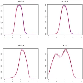
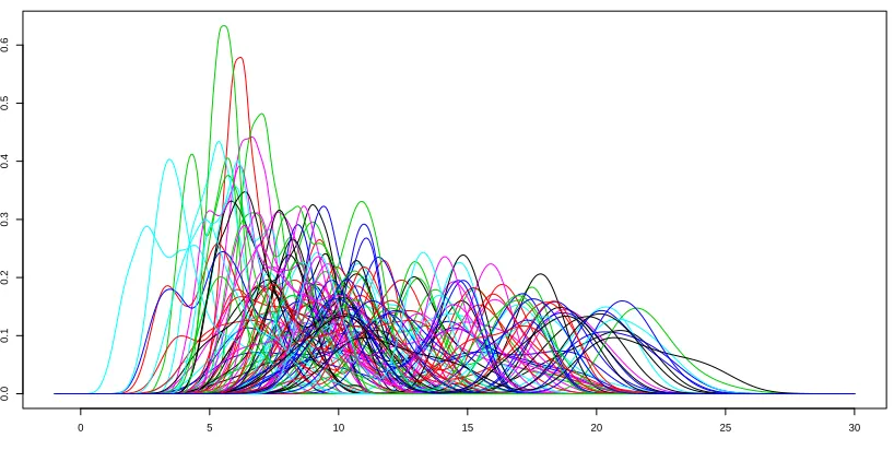
equations (2) and (5). Figure4represents the output forN = 100 points simulated uniformly and independently
in X. Figure 5 represents for different values of x0 the mean (in plain line) and the standard deviation (in
dashed line) of the estimation obtained from the two estimators of the kernel regression in red for L2 norms
and in blue for the Hellinger distance. For these four parameters, the two estimators give approximately the
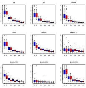
same estimations. Figure6shows the boxplot of the relative error for L2 norms and the Hellinger distance. In
this first example the estimator based on the Hellinger distance seems slightly better than the one based on
the L2 norm. The errors are very close for the norms and the mean but are more different for other quantities
of interest. The variance of the error decreases very quickly for norms. Moreover, the errors are low for most quantities of interest except for 1% and 25% quantiles.
2.1.2. Functional decomposition methods
In this section, the four functional decompositions presented in1.2, MMP with L2 and Hellinger distances,
−1 0 1 2 3
0.0
0.2
0.4
0.6
0.8
1.0
x0 = 0.1
−1 0 1 2 3
0.0
0.2
0.4
0.6
0.8
1.0
x0 = 0.15
−1 0 1 2 3
0.0
0.2
0.4
0.6
0.8
x0 = 0.3
−1 0 1 2 3
0.0
0.1
0.2
0.3
0.4
x0 = 1
Figure 5. Toy example 1: curves in red (resp. blue) plain line represents the estimation of
a density for a fixed x0 from the first (resp. second) method and dashed red (resp. blue)
line represent the standard deviation of the estimation obtained from 25 independent design of experiments. The blue and the red lines are superposed.
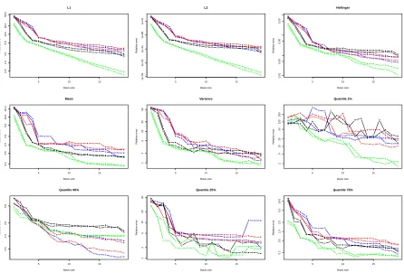
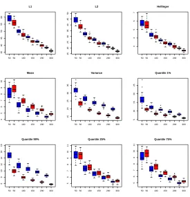
and 100 and for decomposition basis sizes ranging from 1 to 20. The relative errors between the learning
sample functions and their approximations are computed for the 9 quantities of interest. Figure7represents, in
logarithmic scale, these relative errors in function of the basis size for the four decompositions. First, the relative errors are low for all quantities of interest and especially for the norms, the mean and the higher quantiles. For the four decompositions, the relative error for norm decreases very evenly. The decrease is quite regular too for the mean, variance, 75% and 99% quantiles. The quality of approximation of the lower quantiles behaves more irregularly, as it sometimes increases with the basis size. CPCA method outperforms the three others for the three distances. This method seems better for all other quantities of interest except the 25% quantile, but the gap between the decompositions is smaller. The relative error for the learning sample of 100 densities is for most of the quantities higher than the relative error for the sample of 50 densities. For the same number of
components q, it is indeed more difficult to approximate a higher numberN of functions, so that the relative
error increases with the size of the design of experiments for a constant number of components.
Figure 8 represents the L2 relative error of MMP (in red) with N = 200 and the relative error of twenty
independent basis (in black) containing probability functions chosen randomly in the learning samplef1, . . . , fN.
●
● ●
● ● ●
5050 100 150 200 300
6.0
6.5
7.0
7.5
8.0
L1
● ● ●
● ● ●
● ● ●
● ●
● ●
5050 100 150 200 300
0.4
0.5
0.6
0.7
0.8
0.9
L2
● ● ●
● ● ● ●
● ● ● ● ● ●
● ●
●
● ● ●
● ●● ● ● ●
●
5050 100 150 200 300
0.2
0.3
0.4
0.5
Hellinger
● ●
● ●
5050 100 150 200 300
1.5
2.0
2.5
3.0
Mean
● ●
●
●
●
5050 100 150 200 300
3.5
4.0
4.5
5.0
5.5
Variance
●
●
●
● ●
●
● ●●
● ● ● ●
● ● ●
5050 100 150 200 300
50
100
150
200
Quantile 1%
● ●
● ●
● ● ●
●
●
5050 100 150 200 300
1.5
2.0
2.5
Quantile 99%
● ●
● ●
● ● ● ●
●
● ●
●
● ● ● ●
5050 100 150 200 300
50
100
150
Quantile 25%
●
●
● ●
5050 100 150 200 300
1.2
1.4
1.6
1.8
Quantile 75%
Figure 6. Toy example 1: boxplot of the errors for different sizes ofN. Blue: estimator given
by L2 norm. Red: estimator given by the Hellinger distance. Results have been averaged with
25 independent experiments. Blue: estimator given by L2 norm. Red: estimator given by the
Hellinger distance.
2.2.
A five-dimensional example (Toy example 2)
Letx= (x1, x2, x3, x4, x5)∈X = [0,1]5. A second toy example is defined as follows:
G(x, N, U1, U2, B) = (x1+ 2x2+U1) sin(3x3−4x4+N) +U2+ 10x5B+ 5
X
i=1
ixi
where
N ∼ N(0,1)
U1 ∼ U([0,1])
U2 ∼ U([1,2])
B ∼ Bern(1/2).
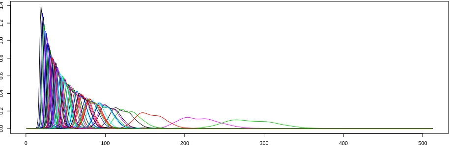
Figure9 represents the output forN = 100 points simulated uniformly and independently inX.
2.2.1. Kernel regression
In this section, the kernel regression is tested on this second toy example with isotropic (Figure 11) and
● ● ● ● ● ● ● ● ● ● ● ● ● ● ● ● ● ● ●
5 10 15
0.5 1.0 2.0 5.0 10.0 20.0 50.0 L1 Basis size Relativ e error ● ● ● ● ● ● ● ● ● ● ● ● ● ● ● ● ● ● ● ● ● ● ● ● ● ● ● ● ● ● ● ● ● ● ● ● ● ● ● ● ● ● ● ● ● ● ● ● ● ● ● ● ● ● ● ● ● ● ● ● ● ● ● ● ● ● ● ● ● ● ● ● ● ● ● ● ● ● ● ● ● ● ● ● ● ● ● ● ● ● ● ● ● ● ● ● ● ● ● ● ● ● ● ● ● ● ● ● ● ● ● ● ● ● ● ● ● ● ● ● ● ● ● ● ● ● ● ● ● ● ● ● ● ● ● ● ● ● ● ● ● ● ● ● ● ● ● ● ● ● ● ●
5 10 15
1e−03 1e−02 1e−01 1e+00 1e+01 L2 Basis size Relativ e error ● ● ● ● ● ● ● ● ● ● ● ● ● ● ● ● ● ● ● ● ● ● ● ● ● ● ● ● ● ● ● ● ● ● ● ● ● ● ● ● ● ● ● ● ● ● ● ● ● ● ● ● ● ● ● ● ● ● ● ● ● ● ● ● ● ● ● ● ● ● ● ● ● ● ● ● ● ● ● ● ● ● ● ● ● ● ● ● ● ● ● ● ● ● ● ● ● ● ● ● ● ● ● ● ● ● ● ● ● ● ● ● ● ● ● ● ● ● ● ● ● ● ● ● ● ● ● ● ● ● ● ● ● ● ● ● ● ● ● ● ● ● ● ● ● ● ● ● ● ● ● ●
5 10 15
0.01 0.05 0.50 5.00 Hellinger Basis size Relativ e error ● ● ● ● ● ● ● ● ● ● ● ● ● ● ● ● ● ● ● ● ● ● ● ● ● ● ● ● ● ● ● ● ● ● ● ● ● ● ● ● ● ● ● ● ● ● ● ● ● ● ● ● ● ● ● ● ● ● ● ● ● ● ● ● ● ● ● ● ● ● ● ● ● ● ● ● ● ● ● ● ● ● ● ● ● ● ● ● ● ● ● ● ● ● ● ● ● ● ● ● ● ● ● ● ● ● ● ● ● ● ● ● ● ● ● ● ● ● ● ● ● ● ● ● ● ● ● ● ● ● ● ● ● ● ● ● ● ● ● ● ● ● ● ● ● ● ● ● ● ● ● ●
5 10 15
0.2 0.5 1.0 2.0 5.0 10.0 20.0 Mean Basis size Relativ e error ● ● ● ● ● ● ● ● ● ● ● ● ● ● ● ● ● ● ● ● ● ● ● ● ● ● ● ● ● ● ● ● ● ● ● ● ● ● ● ● ● ● ● ● ● ● ● ● ● ● ● ● ● ● ● ● ● ● ● ● ● ● ● ● ● ● ● ● ● ● ● ● ● ● ● ● ● ● ● ● ● ● ● ● ● ● ● ● ● ● ● ● ● ● ● ● ● ● ● ● ● ● ● ● ● ● ● ● ● ● ● ● ● ● ● ● ● ● ● ● ● ● ● ● ● ● ● ● ● ● ● ● ● ● ● ● ● ● ● ● ● ● ● ● ● ● ● ● ● ● ● ●
5 10 15
1 2 5 10 20 50 Variance Basis size Relativ e error ● ● ● ● ● ● ● ● ● ● ● ● ● ● ● ● ● ● ● ● ● ● ● ● ● ● ● ● ● ● ● ● ● ● ● ● ● ● ● ● ● ● ● ● ● ● ● ● ● ● ● ● ● ● ● ● ● ● ● ● ● ● ● ● ● ● ● ● ● ● ● ● ● ● ● ● ● ● ● ● ● ● ● ● ● ● ● ● ● ● ● ● ● ● ● ● ● ● ● ● ● ● ● ● ● ● ● ● ● ● ● ● ● ● ● ● ● ● ● ● ● ● ● ● ● ● ● ● ● ● ● ● ● ● ● ● ● ● ● ● ● ● ● ● ● ● ● ● ● ● ● ●
5 10 15
2 5 10 20 50 100 200 Quantile 1% Basis size Relativ e error ● ● ● ● ● ● ● ● ● ● ● ● ● ● ● ● ● ● ● ● ● ● ● ● ● ● ● ● ● ● ● ● ● ● ● ● ● ● ● ● ● ● ● ● ● ● ● ● ● ● ● ● ● ● ● ● ● ● ● ● ● ● ● ● ● ● ● ● ● ● ● ● ● ● ● ● ● ● ● ● ● ● ● ● ● ● ● ● ● ● ● ● ● ● ● ● ● ● ● ● ● ● ● ● ● ● ● ● ● ● ● ● ● ● ● ● ● ● ● ● ● ● ● ● ● ● ● ● ● ● ● ● ● ● ● ● ● ● ● ● ● ● ● ● ● ● ● ● ● ● ● ●
5 10 15
0.5 1.0 2.0 5.0 Quantile 99% Basis size Relativ e error ● ● ● ● ● ● ● ● ● ● ● ● ● ● ● ● ● ● ● ● ● ● ● ● ● ● ● ● ● ● ● ● ● ● ● ● ● ● ● ● ● ● ● ● ● ● ● ● ● ● ● ● ● ● ● ● ● ● ● ● ● ● ● ● ● ● ● ● ● ● ● ● ● ● ● ● ● ● ● ● ● ● ● ● ● ● ● ● ● ● ● ● ● ● ● ● ● ● ● ● ● ● ● ● ● ● ● ● ● ● ● ● ● ● ● ● ● ● ● ● ● ● ● ● ● ● ● ● ● ● ● ● ● ● ● ● ● ● ● ● ● ● ● ● ● ● ● ● ● ● ● ●
5 10 15
1 2 5 10 20 50 Quantile 25% Basis size Relativ e error ● ● ● ● ● ● ● ● ● ● ● ● ● ● ● ● ● ● ● ● ● ● ● ● ● ● ● ● ● ● ● ● ● ● ● ● ● ● ● ● ● ● ● ● ● ● ● ● ● ● ● ● ● ● ● ● ● ● ● ● ● ● ● ● ● ● ● ● ● ● ● ● ● ● ● ● ● ● ● ● ● ● ● ● ● ● ● ● ● ● ● ● ● ● ● ● ● ● ● ● ● ● ● ● ● ● ● ● ● ● ● ● ● ● ● ● ● ● ● ● ● ● ● ● ● ● ● ● ● ● ● ● ● ● ● ● ● ● ● ● ● ● ● ● ● ● ● ● ● ● ● ●
5 10 15
0.2 0.5 1.0 2.0 5.0 10.0 Quantile 75% Basis size Relativ e error ● ● ● ● ● ● ● ● ● ● ● ● ● ● ● ● ● ● ● ● ● ● ● ● ● ● ● ● ● ● ● ● ● ● ● ● ● ● ● ● ● ● ● ● ● ● ● ● ● ● ● ● ● ● ● ● ● ● ● ● ● ● ● ● ● ● ● ● ● ● ● ● ● ● ● ● ● ● ● ● ● ● ● ● ● ● ● ● ● ● ● ● ● ● ● ● ● ● ● ● ● ● ● ● ● ● ● ● ● ● ● ● ● ● ● ● ● ● ● ● ● ● ● ● ● ● ● ● ● ● ● ● ●
Figure 7. Toy example 1: comparison of the relative error for different quantities in function
of the size of the basisq with a design of experiments of size N = 50 (circles) and 100 (filled
circles). Blue: MMP decomposition given by L2norm. Red: MMP decomposition given by the
Hellinger distance. Black: AQM decomposition. Green: CPCA decomposition.
0 10 20 30 40 50
1
2
5
10
50
Size of the basis
Logar
ithm of the percentage of relativ
e error
Figure 8. Toy example 1: comparison of the L2 relative error obtained with MMP (in red)
0 5 10 15 20 25 30
0.0
0.1
0.2
0.3
0.4
0.5
0.6
Figure 9. Toy example 2: representations of outputs forN = 100 different parameters.
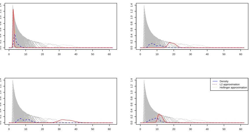
true probability density function (blue dashed line) and the estimation obtained from the two estimators of the kernel regression (red plain line and orange dots line). In this example, the two estimators give different results. In red is represented the relative error for the estimator based on Hellinger distance, in blue for the estimator
based on L2 norm. The Hellinger estimator gives a better approximation of the quantities presented in Figure
11, except for the mean. Contrary to the case of the first toy example, the errors are quite high. The variance
of the error on the norms, presented in Figure 11, is low but does not seem to decrease steadily. The use of
an anisotropic bandwidth does not seem to improve the quality of the estimation, while it is much longer to compute. The errors are approximately the same with isotropic or anisotropic bandwidth. The greater precision brought by the anisotropic bandwidth is compensated by the difficulty to estimate it.
2.2.2. Functional decomposition methods
In this section, the four functional decompositions MMP with L2 and Hellinger distances, AQM and CPCA
are compared. The decompositions are applied to learning samples whose sizes are N = 50 and 100 and for
decomposition basis sizes ranging from 1 to 20. The relative errors between the learning sample functions and
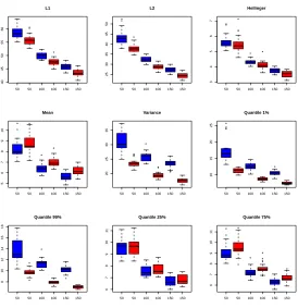
their approximations are computed for the 9 quantities of interest. Figure13 represents, in logarithmic scale,
these relative errors in function of the basis size for the three decompositions. First, the relative errors are low for all quantities of interest, as in the previous example. The relative errors decrease is less even than in the one-dimensional case. The behavior of the errors on 1% and 99% quantiles is particularly unsteady. CPCA
method gives better results than the other methods for L1, L2 norms, 25% and 75% quantiles. However, for all
studied quantities, the AQM and CPCA method seem to give quite equivalent results. MMP method errors are slightly higher than AQM errors for most of the quantities.
3.
Industrial applications
In this section we apply the methods we developed in Section1to three industrial numerical codes of CEA,
0 100 200 300 400
0.0
0.2
0.4
0.6
0 100 200 300 400
0.0
0.2
0.4
0.6
0 100 200 300 400
0.0
0.2
0.4
0.6
0 100 200 300 400
0.0
0.2
0.4
0.6
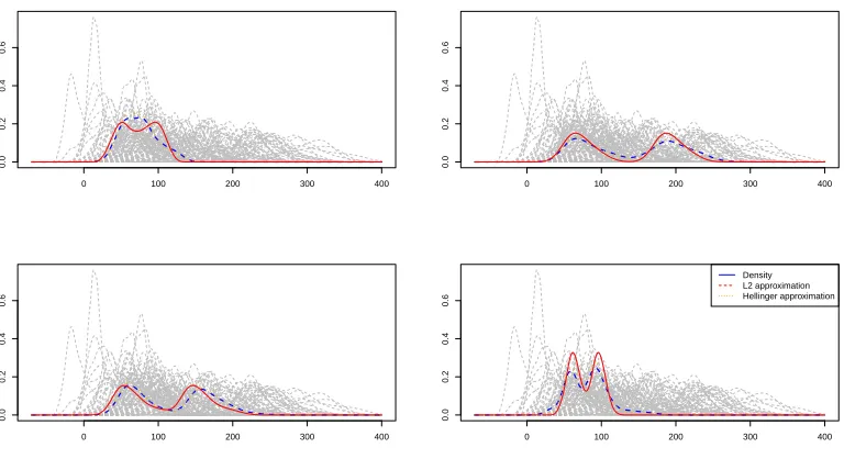
Density L2 approximation Hellinger approximation
Figure 10. Toy example 2: curves in dashed gray lines are probability density functions, red
plain line (resp. orange dots line) represents the estimation of a density for a fixed x0 from
the first (resp. second) method and dashed blue line is the true probability density function.
These estimations were made with h isotropic. The orange dotted line and the red line are
superposed.
3.1.
CEA application: CASTEM test case
3.1.1. Code description
In the framework of nuclear plant risk assessment studies, the evaluation of component reliability during accidental conditions is a major issue required for the safety case. Thermal-hydraulic (T-H) and thermal-mechanic (T-M) system codes model the behaviour of the considered component subjected to highly hypothetic accidental conditions. In the study that we consider here, the T-M code CASTEM takes as input 13 uncertain parameters, related to the initial plant conditions or to the safety system characteristics. Three of them are functional T-H parameters which depend on time: fluid temperature, flow rate and pressure. The other ten parameters are T-M scalar variables. For each set of parameters, CASTEM calculates the absolute mechanical strength of the component and the thermo-mechanical actual applied load. From these two elements, a safety margin (SM) is deduced.
The objective is to assess how these uncertain parameters can affect the code forecasts and more specifically the predicted safety margin. However, CASTEM code is too time expensive to be directly used to conduct uncertainty propagation studies or global sensitivity analysis based on sampling methods. To avoid the problem of huge calculation time, it can be useful to replace CASTEM code by a metamodel. One way to fit a metamodel on CASTEM could be to discretize the functional inputs and to consider the values of the discretization as scalar inputs of CASTEM code. Nevertheless, this solution is often intractable due to the high number of points in
the discretization. To cope with this problem, in [13,17] a method was proposed to treat implicitly these
“uncontrollable” parameters functional parameters, while the other ten scalar parameters are considered as “controllable”. CASTEM output is then a random variable conditionally to “controllable” parameters.
A latin hypercube sampling method [18] is used to build a learning sample of 500 points in dimension 10. For
●
●
5050 100 150 200 300
35
40
45
50
55
60
L1
●
●
● ● ● ●
●
5050 100 150 200 300
15
20
25
30
35
40
45
50
L2
●
●
●
5050 100 150 200 300
3
4
5
6
7
Hellinger
●
5050 100 150 200 300
4
5
6
7
8
9
10
Mean
● ●
● ● ●
5050 100 150 200 300
15
20
25
30
35
Variance
● ●
●
●
5050 100 150 200 300
5
10
15
20
25
Quantile 1%
●
5050 100 150 200 300
6
8
10
12
14
16
18
Quantile 99%
● 5050 100 150 200 300
5
6
7
8
9
10
11
Quantile 25%
● ●● ● ●
5050 100 150 200 300
5
6
7
8
9
10
11
Quantile 75%
Figure 11. Toy example 2: boxplot of the errors for different sizes ofN. Left: estimator given
by L2norm. Right: estimator given by the Hellinger distance. Results have been averaged with
25 independent experiments. These estimations were made with hisotropic. Blue: estimator
given by L2 norm. Red: estimator given by the Hellinger distance.
parameters, randomly chosen in an available database. The probability density functionfi(i= 1, ..,500) of the
safety margin is computed by kernel estimation with the 400 outputs of CASTEM for each set of parameters.
A few examples of the obtained probability density functions are represented on Figure 14. In the following,
the two kernel regression metamodels, then MMP, AQM and CPCA decomposition methods are applied on CASTEM test case.
3.1.2. Kernel regression
In this section, the kernel regression method is applied with isotropic and anisotropic bandwidths. Figure
15 represents for four different values of x0 the true probability density function (blue dashed line) and the
estimation obtained from the two estimators of the kernel regression (L2estimator in red plain line and Hellinger
estimator in orange dotted line), with isotropic bandwidth. One can see that the estimation by the L2estimator
of the four probability density functions is very far from the real function. In particular, at the bottom left of the figure, the mean of the predicted probability function in red is very far from the mean of the real one in dashed blue. On these four probability density functions, the Hellinger estimator gives much better results than
the L2 one.
To verify this first graphical analysis, the Leave-One-Out method has been used to assess the efficiency of the kernel regression-based metamodel. The bandwidth of the kernel regression is estimated thanks to all
probability density functions except theithone. The functionf
iis estimated with the corresponding metamodel
● ●
●
50 50 100 100 150 150
40
45
50
55
60
L1
● ●
●
50 50 100 100 150 150
25
30
35
40
45
50
L2
● ●
● ●
●
● ●
50 50 100 100 150 150
3
4
5
6
7
Hellinger
● ● ●
●
●
50 50 100 100 150 150
5
6
7
8
9
10
Mean
● ● ● ●
●
● ●
● ●
50 50 100 100 150 150
20
25
30
35
Variance
● ● ● ●
●
50 50 100 100 150 150
10
15
20
25
Quantile 1%
●
●
●
●
50 50 100 100 150 150
8
10
12
14
16
18
Quantile 99%
50 50 100 100 150 150
6
7
8
9
10
11
Quantile 25%
● ● ●
●
●
● ● ●
● ●
●
50 50 100 100 150 150
6
7
8
9
10
11
Quantile 75%
Figure 12. Toy example 2: boxplot of the errors for different sizes ofN. Left: estimator given
by L2norm. Right: estimator given by the Hellinger distance. Results have been averaged with
25 independent experiments. These estimations were made withhanisotropic. Blue: estimator
given by L2 norm. Red: estimator given by the Hellinger distance.
repeated for each probability density function in the dataset and all the computed relative errors are averaged.
The mean relative errors of the estimators based on Hellinger distance and L2 norm are given in Table 1 and
Table 2 for the different quantities of interest respectively for an isotropic and anisotropic bandwidths. The
two estimators perform poorly on this dataset. The errors for L1 and L2 norms are particularly high. The
Leave-One-Out validation confirms that the kernel regression method is not adapted to CASTEM test case. This can be explained by the important influence of the controllable T-M parameters compared to the one of the uncontrollable T-H parameters.
3.1.3. Functional decomposition methods
In this section, the four functional decompositions MMP with L2 and Hellinger distances, AQM and CPCA
are compared. Figure16represents, in logarithmic scale, the relative errors on the different norms, modes and
quantiles versus the basis size (from 1 to 20). First, the relative errors are low for all quantities of interest, except for the variance. For the variance, the errors are over 10% with a decomposition basis with 20 functions. The errors for small bases are high but decrease very quickly. The decrease is especially quick and even for
errors on L1, L2 and Hellinger distances. For modes and quantiles, the errors of the four methods do not
decrease steadily for all quantities of interest, and especially for small basis sizes. CPCA clearly outperforms
other methods for the L1, L2and Hellinger distances. For other quantities of interest, it gives good results. For
● ● ● ● ● ● ● ● ● ● ● ● ● ● ● ● ● ● ●
5 10 15
2 5 10 20 50 100 L1 Basis size Relativ e error ● ● ● ● ● ● ● ● ● ● ● ● ● ● ● ● ● ● ● ● ● ● ● ● ● ● ● ● ● ● ● ● ● ● ● ● ● ● ● ● ● ● ● ● ● ● ● ● ● ● ● ● ● ● ● ● ● ● ● ● ● ● ● ● ● ● ● ● ● ● ● ● ● ● ● ● ● ● ● ● ● ● ● ● ● ● ● ● ● ● ● ● ● ● ● ● ● ● ● ● ● ● ● ● ● ● ● ● ● ● ● ● ● ● ● ● ● ● ● ● ● ● ● ● ● ● ● ● ● ● ● ● ● ● ● ● ● ● ● ● ● ● ● ● ● ● ● ● ● ● ● ●
5 10 15
5e−02 5e−01 5e+00 5e+01 L2 Basis size Relativ e error ● ● ● ● ● ● ● ● ● ● ● ● ● ● ● ● ● ● ● ● ● ● ● ● ● ● ● ● ● ● ● ● ● ● ● ● ● ● ● ● ● ● ● ● ● ● ● ● ● ● ● ● ● ● ● ● ● ● ● ● ● ● ● ● ● ● ● ● ● ● ● ● ● ● ● ● ● ● ● ● ● ● ● ● ● ● ● ● ● ● ● ● ● ● ● ● ● ● ● ● ● ● ● ● ● ● ● ● ● ● ● ● ● ● ● ● ● ● ● ● ● ● ● ● ● ● ● ● ● ● ● ● ● ● ● ● ● ● ● ● ● ● ● ● ● ● ● ● ● ● ● ●
5 10 15
0.2 0.5 1.0 2.0 5.0 10.0 Hellinger Basis size Relativ e error ● ● ● ● ● ● ● ● ● ● ● ● ● ● ● ● ● ● ● ● ● ● ● ● ● ● ● ● ● ● ● ● ● ● ● ● ● ● ● ● ● ● ● ● ● ● ● ● ● ● ● ● ● ● ● ● ● ● ● ● ● ● ● ● ● ● ● ● ● ● ● ● ● ● ● ● ● ● ● ● ● ● ● ● ● ● ● ● ● ● ● ● ● ● ● ● ● ● ● ● ● ● ● ● ● ● ● ● ● ● ● ● ● ● ● ● ● ● ● ● ● ● ● ● ● ● ● ● ● ● ● ● ● ● ● ● ● ● ● ● ● ● ● ● ● ● ● ● ● ● ● ●
5 10 15
0.2 0.5 1.0 2.0 5.0 10.0 20.0 Mean Basis size Relativ e error ● ● ● ● ● ● ● ● ● ● ● ● ● ● ● ● ● ● ● ● ● ● ● ● ● ● ● ● ● ● ● ● ● ● ● ● ● ● ● ● ● ● ● ● ● ● ● ● ● ● ● ● ● ● ● ● ● ● ● ● ● ● ● ● ● ● ● ● ● ● ● ● ● ● ● ● ● ● ● ● ● ● ● ● ● ● ● ● ● ● ● ● ● ● ● ● ● ● ● ● ● ● ● ● ● ● ● ● ● ● ● ● ● ● ● ● ● ● ● ● ● ● ● ● ● ● ● ● ● ● ● ● ● ● ● ● ● ● ● ● ● ● ● ● ● ● ● ● ● ● ● ●
5 10 15
10 20 50 100 Variance Basis size Relativ e error ● ● ● ● ● ● ● ● ● ● ● ● ● ● ● ● ● ● ● ● ● ● ● ● ● ● ● ● ● ● ● ● ● ● ● ● ● ● ● ● ● ● ● ● ● ● ● ● ● ● ● ● ● ● ● ● ● ● ● ● ● ● ● ● ● ● ● ● ● ● ● ● ● ● ● ● ● ● ● ● ● ● ● ● ● ● ● ● ● ● ● ● ● ● ● ● ● ● ● ● ● ● ● ● ● ● ● ● ● ● ● ● ● ● ● ● ● ● ● ● ● ● ● ● ● ● ● ● ● ● ● ● ● ● ● ● ● ● ● ● ● ● ● ● ● ● ● ● ● ● ● ●
5 10 15
1 2 5 10 20 50 100 Quantile 1% Basis size Relativ e error ● ● ● ● ● ● ● ● ● ● ● ● ● ● ● ● ● ● ● ● ● ● ● ● ● ● ● ● ● ● ● ● ● ● ● ● ● ● ● ● ● ● ● ● ● ● ● ● ● ● ● ● ● ● ● ● ● ● ● ● ● ● ● ● ● ● ● ● ● ● ● ● ● ● ● ● ● ● ● ● ● ● ● ● ● ● ● ● ● ● ● ● ● ● ● ● ● ● ● ● ● ● ● ● ● ● ● ● ● ● ● ● ● ● ● ● ● ● ● ● ● ● ● ● ● ● ● ● ● ● ● ● ● ● ● ● ● ● ● ● ● ● ● ● ● ● ● ● ● ● ● ●
5 10 15
2 5 10 20 Quantile 99% Basis size Relativ e error ● ● ● ● ● ● ● ● ● ● ● ● ● ● ● ● ● ● ● ● ● ● ● ● ● ● ● ● ● ● ● ● ● ● ● ● ● ● ● ● ● ● ● ● ● ● ● ● ● ● ● ● ● ● ● ● ● ● ● ● ● ● ● ● ● ● ● ● ● ● ● ● ● ● ● ● ● ● ● ● ● ● ● ● ● ● ● ● ● ● ● ● ● ● ● ● ● ● ● ● ● ● ● ● ● ● ● ● ● ● ● ● ● ● ● ● ● ● ● ● ● ● ● ● ● ● ● ● ● ● ● ● ● ● ● ● ● ● ● ● ● ● ● ● ● ● ● ● ● ● ● ●
5 10 15
0.02 0.05 0.20 0.50 2.00 5.00 20.00 Quantile 25% Basis size Relativ e error ● ● ● ● ● ● ● ● ● ● ● ● ● ● ● ● ● ● ● ● ● ● ● ● ● ● ● ● ● ● ● ● ● ● ● ● ● ● ● ● ● ● ● ● ● ● ● ● ● ● ● ● ● ● ● ● ● ● ● ● ● ● ● ● ● ● ● ● ● ● ● ● ● ● ● ● ● ● ● ● ● ● ● ● ● ● ● ● ● ● ● ● ● ● ● ● ● ● ● ● ● ● ● ● ● ● ● ● ● ● ● ● ● ● ● ● ● ● ● ● ● ● ● ● ● ● ● ● ● ● ● ● ● ● ● ● ● ● ● ● ● ● ● ● ● ● ● ● ● ● ● ●
5 10 15
0.2 0.5 1.0 2.0 5.0 10.0 20.0 Quantile 75% Basis size Relativ e error ● ● ● ● ● ● ● ● ● ● ● ● ● ● ● ● ● ● ● ● ● ● ● ● ● ● ● ● ● ● ● ● ● ● ● ● ● ● ● ● ● ● ● ● ● ● ● ● ● ● ● ● ● ● ● ● ● ● ● ● ● ● ● ● ● ● ● ● ● ● ● ● ● ● ● ● ● ● ● ● ● ● ● ● ● ● ● ● ● ● ● ● ● ● ● ● ● ● ● ● ● ● ● ● ● ● ● ● ● ● ● ● ● ● ● ● ● ● ● ● ● ● ● ● ● ● ● ● ● ● ● ● ●
Figure 13. Toy example 2: comparison of the relative error for different quantities in function
of the size of the basisq with a design of experiments of size N = 50 (circles) and 100 (filled
circles). Blue: MMP decomposition given by L2norm. Red: MMP decomposition given by the
Hellinger distance. Black: AQM decomposition. Green: CPCA decomposition.
0 100 200 300 400 500
0.0 0.2 0.4 0.6 0.8 1.0 1.2 1.4