Iranian Journal of Electrical and Electronic Engineering, Vol. 16, No. 1, March 2020 85
IS-MRAS With On-Line Adaptation Parameters Based on
Type-2 Fuzzy LOGIC for Sensorless Control of IM
B. Yassine*(C.A.), Z. Fatiha** and L. Chrifi-Alaoui***
Abstract: This paper suggests novel sensorless speed estimation for an induction motor (IM) based on a stator current model reference adaptive system (IS-MRAS) scheme. The IS-MRAS scheme uses the error between the reference and estimated stator current vectors and the rotor speed. Observing rotor flux and the speed estimating using the conventional MRAS technique is confronted with certain problems related to the presence of the pure integrator and the rotor resistance causing offsets at low speeds, as proved by the most recent publications. These offsets are disastrous in sensorless control since these signals are no longer suitable to calculate of park angle (θs). This paper discusses the new MRAS approach (IS-MRAS) for on-line identification of the rotor resistance suitable for compensating offsets and solving problems of ordinary MRAS at low speed. This new MRAS approach used to estimate the components of the rotor flux and rotor speed without using the voltage model with on-line Setting parameters (Kp, K1) based on Type-2 fuzzy Logic. The results of the simulation and the experimental results are presented and show the effectiveness of the proposed technique.
Keywords: Induction Motor, IS-MRAS, Type-2 Fuzzy logic, Sensorless Control.
1 Introduction1
HE asynchronous machine, by its construction, is the most robust machine and least costly. The advances made in control and the considerable technological advances in both the power electronics and microelectronics have made it possible to install the powerful controls of this machine, making it a dreadful concurrent in the sectors of variable speed.
However, many problems remain, since the variation of the parameters of the machine, the presence of the mechanical sensor and the degraded operation are all difficulties that have emulated the eagerness of the
Iranian Journal of Electrical and Electronic Engineering, 2020. Paper first received 29 July 2019, revised 30 October 2019, and accepted 01 November 2019.
* The author is with the Department of Electrical Engineering, University of Khenchela, Algeria.
E-mail: [email protected].
** The author is with the Department of Electrical Engineering, Laboratory LSPIE, University of Batna-2, Algeria.
E-mail: [email protected].
*** The author is with the Laboratoire des Technologies Innovantes (LTI,EA 3899), France.
E-mail: [email protected]. Corresponding Author: B. Yassine.
researchers, as proved by the ever-increasing number of publications that study the subject, [1-22].
Control of induction machine (IM) requires the installation of an incremental encoder for the speed measure. The use of this encoder results in an additional cost which may be greater than that of the machine and especially in the case of low power machines. However, the reliability of the system decreases because of this fragile device which in turn requires special maintenance.
That is why the idea of eliminating the incremental encoder has arisen and that the research on the sensorless control of the asynchronous machine is begun and is continuously expanding.
Several strategies have been proposed in the literature to achieve this object. A large part of the proposed methods is based on observers depending on the machine model.
Unfortunately, these techniques fail to replace the incremental encoder in the low-speed range and also during the presence of disturbances such as the load application; this consists of the essential problem of these techniques. Other research is based on the contribution of artificial intelligence to improve machine sensorless control. Among them, we can
T
Iranian Journal of Electrical and Electronic Engineering, Vol. 16, No. 1, March 2020 86 highlight methods by sliding mode [4, 5], using a new
concept of stator resistance [19], and many adaptive methods (MRAS) have been proposed such as [1-3], [6, 7], [9-11], [21, 22]. However, rotor flux MRAS first introduced by Schauder [2], the MRAS strategy remains the most popular, and a lot of effort has been focused on improving its performance, the results obtained by these authors confirm, indeed, the disadvantages of this technique which are the sensitivity to the variation of the parameters, in particular to the rotor resistance, and pure integration problems, which limit its performance at low and zero speed regions of operation.
In this paper, we propose a new MRAS approach with the on-line adaptation of the speed estimation mechanism parameters, moreover, we propose the on-line estimation of the rotor resistance.
The type-2 fuzzy logic was used to supervise the variations of Kp and Ki of the speed estimator.
The Novelty in this paper is the elimination of the voltage model, because the conventional MRAS technique is confronted with certain problems related to the presence of the pure integrator in the voltage model causing offsets at low speeds, this offsets are disastrous in control since these signals are no longer suitable to calculate of park angle (θs).
The validity of the proposed method is verified using simulation and experimentation. Moreover, the sensorless control of the asynchronous machine associated with the static converter presents several difficulties in terms of performance, in this context the use of type-2 fuzzy logic constitutes an interesting alternative for improving the performance of the new approach of MRAS observer in low speed.
2 Asynchronous Motor Model
We consider two mathematical models, the first is used to realize the control vector and the second is used to synthesize observer.
Model related to the rotating field (dq-coordinates):
1 1 1 1 1 1 . sdsd s sq rd rq sd
s s r r s
sq
sq s sd rq rd sq
s s r r s
rd
sd rd s rq
r r
rq
sq rq s rd
r r
e sq rd sd rq
r
di R M
i i V
dt L L L T L
di R M
i i V
dt L L L T L
d M
i
dt T T
d M
i
dt T T
p M
T i i
L (1)
In the stationary reference frame (αβ-coordinates), the dynamic model of a 3-phase induction motor can be described as
1
1
r r s
s s s s
r r s
s s s s
r
s r r
r r
r
s r r
r r
d L di
V R i L
dt M dt
d L di
V R i L
dt M dt
d M
i
dt T T
d M
i
dt T T
(2) where 2 2 2
1 , , r
r r
s r r r
L
M M
R T
L L L R
where Vs is the stator voltage, Vris the rotor voltage, Rs
is the stator resistance, Rris the rotor resistance, ω is the
electrical angular frequency, φs is the stator flux, φr is
the rotor flux power and Ls, M, and Lr are the stators,
magnetizing, and rotor inductances, respectively.
3 Vector Control
To test the proposed approach, we use indirect vector control as shown in Fig 2. We take Vsd and Vsq as
control variables. In this context and for φrq = 0, the
equations system (1) becomes:
1 .
sd
sd s sd s s sq rd
r r
di M
V L R i L i
dt L T
(3)
R. sq
sq s sq s s sd rd
r
di M
V L i L i
dt L
(4)
sq s rd
r M i
T (5)
. rd
r rd sd
d
T M i
dt (6)
3 2e rd sq
r pM
C i
L
(7)
where Ce is the electromagnetic torque.
Expression (6) shows that the rotor flux evolution follows the stator current, furthermore, the torque of (7) is similar to that to DC motor because isd and isq are
continuous components. It can be said that with the field orientation, the torque control becomes linear and adjustable by acting on isq when the flux φdr is kept
constant. If the flux φrd is replaced by the reference flux
φr*, the developed torque given by (7) can be rewritten
as follows:
*
e r sq
C k i (8)
where 3 2 r
pM k
L
and φr* is the rotor flux reference.
From (5), we deduce the Park angle:
Iranian Journal of Electrical and Electronic Engineering, Vol. 16, No. 1, March 2020 87 sq s s r rd Mi dt dt T
(9)The decoupling by compensation as follows:
*
sd sd sd
V V e (10)
*
sq sq sq
V V e (11)
where
sd s s sq
r r M
e L i
T L
(12)
*
sq s s sd
r M
e L i
L
(13)
* sd
sd s sd
di
V L Ri
dt
(14)
* sq
sq s sq
di
V L Ri
dt
(15)
From new components Vsd* and Vsq*, we deduce the
control components Vsd and Vsq.
4 Classical MRAS Observer
The MRAS observer analyzed two independent equations for the derivative time of the rotor flux vector, obtained from (2). They are usually referred to as the “voltage model” called reference model and “current model” called adjustable model and they are given, respectively, by
r r s
s s s s
r r s
s s s s
d L di
V R i L
dt M dt
d L di
V R i L
dt M dt
(16)
and we propose the following current reference model:
1
1 r
s r r
r r
r
s r r
r r
d M
i
dt T T
d M
i
dt T T
(17)
the model (17) can be written in an adjustable form:
1
1 ˆ
ˆ ˆ ˆ
ˆ
ˆ ˆ ˆ r
s r r
r r
r
s r r
r r
d M
i
dt T T
d M
i
dt T T
(18)
where ˆr is the estimated rotor flux and ˆ is estimated rotor speed.
The dynamic equation of the estimation error εαβ is
obtained by subtracting (17) and (18).
1 ˆ ˆ
ˆ 1 ˆ r r r r d dt T d dt T (19)
where ˆ
ˆ r r r r .
For the correctness of the parameter technique, it must be ensured that the system (19) is stable. It naturally requires the error (εαβ) tends to be zero. The stability of
this algorithm is studied, using the hyper-stability Popov criterion.
The system (19) can be written in the following matrix form: d A C dt
(20)
where _ _ 1 ˆ ˆ
0 ( ).
and ˆ
1 ( ˆ). 0
r aj r r aj r T A C T
We consider the adaptation law proposed by [11]:
2 1
0
ˆ ( ) ( )
t
f f d
(21)The criterion of Popov requires that:
1 2 0 1 0 ; 0 t T
C dt t
(22)where γ02 is a positive constant. The solution of (22) proposed by [10] is:
1 2 ˆ . . . . ˆ ˆ ˆi r r r f r
p r r r f r
f K f K
(23)
By replacing (23) in (21), we obtain the speed estimation:
0
ˆ .ˆ .
.
ˆ ˆ
.
ˆ
p r r r f r
t
i r r r f r
K K dt
(24)where Kp and Ki are positive gains.
However, the main problem of the classical MRAS observer is its poor estimation at low speeds [6], [9-11], [21, 23]. That is why we present a new MRAS speed observer in the following paragraph.
5 Stator Current Model Reference Adaptive System (IS-MRAS)
The proposed MRAS is using the current model only.
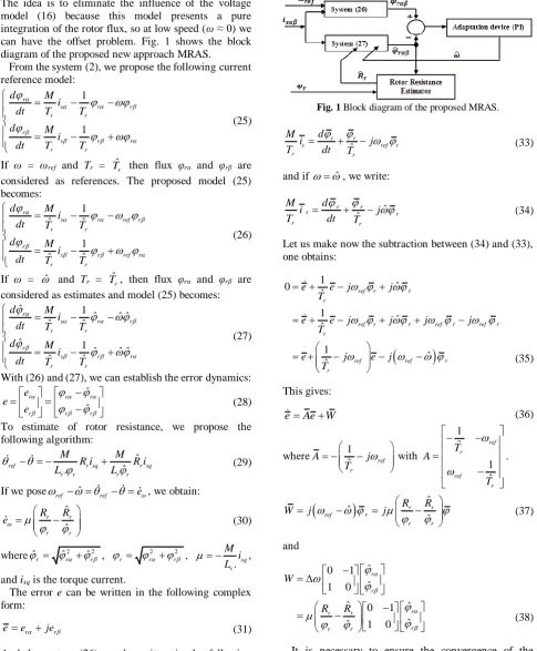
Iranian Journal of Electrical and Electronic Engineering, Vol. 16, No. 1, March 2020 88 The idea is to eliminate the influence of the voltage
model (16) because this model presents a pure integration of the rotor flux, so at low speed (ω ≈ 0) we can have the offset problem. Fig. 1 shows the block diagram of the proposed new approach MRAS.
From the system (2), we propose the following current reference model:
1
1 r
s r r
r r
r
s r r
r r
d M
i
dt T T
d M
i
dt T T
(25)
If ω = ωref and Tr = ˆTr then flux φrα and φrβ are
considered as references. The proposed model (25) becomes: ˆ ˆ 1 1 ˆ ˆ r
s r ref r
r r
r
s r ref r
r r
d M
i
dt T T
d M
i
dt T T
(26)
If ω = ˆ and Tr = ˆTr, then flux φrα and φrβ are considered as estimates and model (25) becomes:
ˆ
ˆ ˆ ˆ
ˆ ˆ
ˆ
ˆ ˆ ˆ
ˆ ˆ
1
1 r
s r r
r r
r
s r r
r r
d M
i
dt T T
d M
i
dt T T
(27)
With (26) and (27), we can establish the error dynamics: ˆ
ˆ
r r r
r r r
e e e
(28)
To estimate of rotor resistance, we propose the following algorithm:
.
ˆ ˆ
ref r sq r sq
r r r r
M M
R i R i
L L
(29)
If we poseref ˆ ref e, we obtain: ˆ
ˆ
r r
r r
R R
e
(30)
whereˆr ˆr2 ˆr2 ,
2 2
r r r
, .sq r M i L , and isq is the torque current.
The error e can be written in the following complex form:
r r
ee je (31)
And the system (26) can be written in the following complex form: ˆ r r s r r r d M i j
T dt T
(32)
If ω = ωref, we write:
Fig. 1 Block diagram of the proposed MRAS.
ˆ
r r
s ref r
r r
d M
i j
T dt T
(33)
and if ˆ, we write: ˆ ˆ r r s r r r d M i j
T dt T
(34)
Let us make now the subtraction between (34) and (33), one obtains:
˙ ˆ ˆ ˆ ˆ ˆ ˆ 1 0 1 1 r ref r rr r r
ref r ref ref
r
r
ref ref
r
e e j j
T
e e j j j j
T
e j e j
T
(35)
This gives:
e Ae W (36)
where 1ˆ ref r
A j
T
with
ˆ ˆ 1 1 ref r ref r T A T .
ˆ
ˆˆ r r r ref r r R R
W j j
(37)
and 0 1 1 0 0 ˆ ˆ ˆ ˆ ˆ ˆ 1 1 0 r r r r r r r r W R R
(38)
It is necessary to ensure the convergence of the estimation error towards zero, so we have to make sure that the system (34) is stable, the stability of this algorithm is studied using the hyperstability Popov criterion. Indeed, the derivation of the error is composed of two terms. The first is linear and the second is nonlinear.
Iranian Journal of Electrical and Electronic Engineering, Vol. 16, No. 1, March 2020 89 We define the following Lyapunov function:
2ˆ 0 2
ref T
V e e
(39)
where γ is a positive constant.
The function given in (34) is globally negative definite. Thus, V0 ˆ.
The time derivative of the Lyapunov function becomes:
21 1
2 2
T T d e
V e e e e
dt
Let us replace by its value:
1 2
1 2
1 2
T T
T T T T T
T T T
d
V Ae W e Ae W
dt d
e A e W e e Ae e W
dt
d de
e A A e e W
P
e
e
dt dt
Q
(40)
Where
1 ˆ
1
1 1
1 1
2 2
1 0
1
0
ˆ
ˆ
ˆ 1
ˆ
0
ref ref
r r
T
ref ref
r r
r
T T
Q A A
T T
T
The first term of (40) is negative. If P = 0, then:
T d
e W
dt
(41)
ˆ
ˆ r
r r
r R R
(42)
where
ˆ
ˆ ˆ
ˆ
ˆ ˆ
r T
r r r r
r
r r r r
e W
(43)
We replace (43) into (41), we obtain:
ˆ
ˆ ˆ
r r r r
d
dt
ˆ r ˆr rˆr dt
(44)To improve the precision amounts adding a proportional gain to the integral action (Kp, Ki).
ˆ Kp rˆr rˆr Ki rˆr rˆr dt
.According to equation (42) and (44), we can see that the estimated resistance depends on the estimated flux, therefore, it is not possible to obtain correct simultaneous speed and rotor resistance estimation. In order to overcome this problem and to obtain simultaneousˆand ˆRrestimation, a small initial value is added to the estimated rotor flux. Once the estimate is obtained, we disable this value.
0
ˆ
ˆ r
r r
r
R R R
(45)
The block diagram of speed sensorless field-oriented using the new approach MRAS is presented in Fig. 2.
6 Type-2 Fuzzy Adapter 6.1 Interval type-2 Fuzzy
The interval type-2 fuzzy logic is depicted in Fig. 3. We discuss briefly the operation of each component of the FLC, with emphasis on type-reduction.
Fuzzifier
The fuzzifier maps a crisp input into the interval type-2 membership functions to produce a set of interval type-1 fuzzy sets. The number of sets depends on the number of inputs and membership functions. Singleton fuzzification was chosen due to its facility of implementation. Using singleton fuzzification two membership values are calculated for each fuzzy set i.e. the lower () and upper () membership values.
Inference Engine
As in type-1 fuzzy logic, the inference is the logical operation by which a proposition is admitted by virtue of its liaison with other propositions held to be true. Only in type-2 fuzzy logic is used the type-2 fuzzy base rule. To carry out a relation between an input vector x = {x1, x2, …, xp} and the output (y), the activation
Fig. 2 Sensorless field-oriented control scheme.
Iranian Journal of Electrical and Electronic Engineering, Vol. 16, No. 1, March 2020 90 interval associated with the first outputs fuzzy set is
calculated by the following equation:
1
( )
l i
p
i f i
x
(46)where l( )
i i
f x
is the activation interval associated with the variable xi.
The fuzzy set of the output corresponding to the first rule is computed using the t-norm operator () as follows:
1
( ) ( ) ( )
l l l
i
p
i
B G F
i
y y x
(47)Since only the interval type-2 fuzzy logic sets are used and the t-standard-product operation is implemented, then the activation interval associated with the first set of output defined by:
inf sup
( ) [ ( ), ( )]
i i i
F x f x f x (48)
1 2
inf ( ) iinf( )1 iinf( 2) ... iinf( )
p
i
p
F F F
f x x x x (49)
1 2
sup( ) isup( )1 isup( 2) ... isup( )
p
i
p
F F F
f x x x x (50)
The terms iinf( )
p i
F x
and isup( )
p i
F x
are respectively the lower and upper values of the interval activation corresponding to i( )
p p
F x
.
Rules
The difference between the rules of a type-1 fuzzy logic system and those of type-2 will reside only in the nature of membership functions, therefore, the rules structure in the case of type-2 remains exactly the same as that of type-1, The only difference being that some membership functions will be type-2, Then the i-th rule of a type-2 fuzzy system will have the following form [23-26]:
1 1 2 2
IF is x Fi and is x Fi .. xp is Fpi THEN is y Gi (51) Generally, the fuzzy rules are organized using tables which objective is to represent all the different combinations among the inputs of the system. The structure of the rule-base does not vary between type-1 and type-2 fuzzy logic.
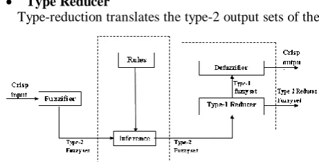
Type Reducer
Type-reduction translates the type-2 output sets of the
Fig. 3 Type-2 fuzzy Logic system Structure.
inference engine to a type-1 set; this is called a type reduced set. These type-reduced sets are then defuzzified to obtain a crisp output used for control. We will use the “center-of-sets” type reduction, as it has reasonable computational complexity lying between Computationally expensive centroid type-reduction and the simple height and modified height type-reductions which have problems when only one rule fires. The type reduced set using the “center-of-sets” type-reduction is expressed below [23]:
1 1
1 2 1 1
1
( , ,.., , ,.., ) ... .. ... 1 /
M M
M i i
M M i
M i
z z w w
i w z
Y Z Z Z W W
w
(52)Since each set in (52) is a fuzzy set (type-1 interval), then (Y) is also a fuzzy set (interval type-1) that is the domain is located on the real axis:
1 2 1
( , ,.., M, ,.., M) l, r
Y Z Z Z W W y y (53)
where, the type reduced set Y is an interval set defined by its left and right most points y1, yr, [ inf, sup]
i i i
z z z ,
[ , ]
i i i
l r
w w w is the centroid of the type-2 interval consequent set i
G , whose details are given in [23], and i = 1, …, M.
Defuzzifier
The defuzzification consists in transforming the type-reduced fuzzy set into a crisp output. It is the simplest subsystem, the crisp output value is computed as the average of the bounds of the type-reduced set.
2
l r
y y
Y (54)
with
1 1
1 1
,
M M
i i i i
l l r r
i i
l M r M
i i
l r
i i
w z w z
y y
w w
(55)Using the Karnik-Mendel algorithm To calculate these two points [23, 24].
6.2 Type-2 FLA Design of New Approach MRAS The inputs of the adapter are the speed error and its variation. The adaptations made on the parameters of the PI regulator aim at correcting progressively the evolution of the system by acting on the regulation law. During the on-line operation of the regulator, a fuzzy matrix makes it possible to adapt the gains so as to optimize the characteristics of the temporal response. A rule base is designed, allowing as input variables e and Δe as output variables the variation rates K1 and K2 which must be added at each instant to the nominal
Iranian Journal of Electrical and Electronic Engineering, Vol. 16, No. 1, March 2020 91 parameters
0
p K and
0
ip
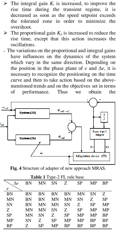
K , as shown in (58) and (59). The decision table is extracted from an expertise obtained following several simulation tests. Fig. 4 shows the structure of the adapter.
ˆ
ref
e (56)
de e
dt
(57)
0
1
p p
K K K (58)
0
2
i ip
K K K (59)
Design of the Rule Base
To determine the basis of the rules, it is necessary to rely on considerations between the evolution of the PI parameters and the desired performance. To determine the basis of the rules, it is necessary to rely on considerations between the evolution of the parameters of the PI controller and the desired performance:
The integral gain Ki is increased, to improve the
rise time during the transient regime, it is decreased as soon as the speed setpoint exceeds the tolerated zone in order to minimize the overshoot.
The proportional gain Kp is increased to reduce the
rise time, except that this action increases the oscillations.
The variations on the proportional and integral gains have influences on the dynamics of the system which vary in the same direction. Depending on the position in the phase plane of e and Δe, it is necessary to recognize the positioning on the time curve and then to take action based on the above-mentioned trends and on the objectives set in terms of performance. Thus we obtain the
Fig. 4 Structure of adapter of new approach MRAS.
Table 1 Type-2 FL rule base. Δe
e
BN MN SN Z SP MP BP
BN BN BN BN BN MN SN Z
MN BN BN MN MN SN Z SP
SN BN MN MN SN Z SP MP
Z MN MN SN Z SP MP MP
SP MN SN Z SP MP MP BP
MP SN Z SP MP MP BP BP
BP Z SP MP BP BP BP BP
rules base illustrated by Table 1.
The membership functions of the input variables are shown in Fig. 5. Fig. 6 shows the general structure of a type-2 FLA, The only difference with type-1 is located at the output processing system.
7 Simulation and Experimental Results
The presented technique was initially verified using computer simulations. The simulations of the speed controlled FOC system with MRAS speed estimator and proposed Rr estimator are performed in MATLAB,
Simulink Toolbox.
Fig. 20 shows the DSP based implementation of the speed sensorless IFOC control. The sampling frequency is fixed at 10kHz and the controller receives the stator currents measurements through two 8-bit A/D converters. Then, using the PWM technique, the reference voltages are sent to the machine via the voltage-source inverter whose switching frequency is fixed at 10kHz. Parameters of induction motor are Rs = 5.72Ω, Rs = 4.2Ω, Ls = Lr = 0.462H, M = 0.44H,
J = 0.0049Kg.m2, f = 0.003NM/rad, p = 2. 7.1 Simulation Results
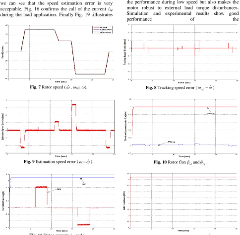
The sensorless field-oriented control (FOC) induction motor drive, shown in Fig. 2, is used where the actual speed feedback signal is replaced by the estimated speed signal. Fig. 7 actual speed (ω), estimated speed (ˆ ) and reference speed (ωref). We see in Fig.8 that the tracking
speed error (ωref–ˆ) is small even at zero speed regions
and converge quickly to zero, also, in Fig.9 we can see that the speed estimation error (ω–ˆ) is acceptable. To test the robustness toward load torque for a speed reference. The step load of 5Nm is applied between t = 4.2s and t = 7.2s, we can see, after very small variation of speed estimation error and speed tracking error, therefore, this disturbance does not affect system performance. We can see in Fig. 10 that the flux ( ˆrd) installs correctly and the q-axis flux (ˆrq) is maintained at zero value, which confirms the field orientation.
Fig. 5 Membership functions.
Fig. 6 General structure of Type-2 FLA.
Iranian Journal of Electrical and Electronic Engineering, Vol. 16, No. 1, March 2020 92 All these results confirm the efficiency of our new
approach observer and control. Fig.11 shows the direct and quadratic stator currents (isd, isq). Fig. 12 shows the
correct estimate of the rotor resistance.
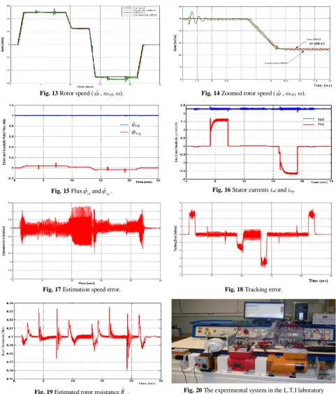
7.2 Experimental Results
Fig. 13 shows the performance of the speed estimation. This estimated speed is used in the new approach of the MRAS observer. We notice that the estimated speed is in agreement with the real speed.
Fig. 15 shows the flux ˆrdis established correctly and follows the reference value, the quadric fluxˆrqis practically nil, this confirms the vector control by decoupling. Fig. 18 shows that the tracking speed error is small and converges quickly to zero, also, in Fig. 17 we can see that the speed estimation error is very acceptable. Fig. 16 confirms the call of the current isq
during the load application. Finally Fig. 19 .illustrates
the correct estimation of the rotor resistance ˆRr. All these Experimental results confirm the efficiency of the sensorless speed estimation for an induction motor (IM) based on the proposed observer.
8 Conclusion
This paper discusses the new approach MRAS (IS-MRAS) and rotor resistance estimation for speed sensorless control induction motor with on-line adaptation parameters. A novel adaptation mechanism using type-2 fuzzy logic controller, which replaces conventionally used PI controller in the adaptation mechanism. The speed estimation using the PI controller deteriorates at low speeds and hence proposed a T2FLC based speed observer that not only improves the performance during low speed but also makes the motor robust to external load torque disturbances. Simulation and experimental results show good
performance of the
Fig. 7 Rotor speed ( ˆ, ωref, ω). Fig. 8 Tracking speed error (ref ˆ).
Fig. 9 Estimation speed error ( ˆ). Fig. 10 Rotor flux ˆrdand ˆrq.
Fig. 11 Stator currents isd and isq. Fig. 12 Estimated rotor resistance ˆ
r
R .
Iranian Journal of Electrical and Electronic Engineering, Vol. 16, No. 1, March 2020 93
Fig. 13 Rotor speed ( ˆ, ωref, ω). Fig. 14 Zoomed rotor speed ( ˆ, ωref, ω).
Fig. 15 Flux ˆrdand ˆrq. Fig. 16 Stator currents isd and isq.
Fig. 17 Estimation speed error. Fig. 18 Tracking error.
Fig. 19 Estimated rotor resistance ˆRr. Fig. 20 The experimental system in the L.T.I laboratory
(University of Picardie, I.U.T of AISNE, 02880 CUFFIES) consisting of a 1.5kW induction motor, a voltage-source inverter,
and a digital signal processor (DSP). sensorless control at low speed. Sensorless control of
induction motor with on-line resistance estimation allows seeing the rotoric resistance variation in external load torque disturbances.
References
[1] A. R. Teja, C. Chakraborty, S. Maiti, and Y. Hori, “A new model reference adaptive controller for four quadrant vector controlled induction motor drives,” IEEE Transactions on Industrial Electronics, Vol. 59, No. 10, 2012.
Iranian Journal of Electrical and Electronic Engineering, Vol. 16, No. 1, March 2020 94 [2] C. Schauder, “Adaptive speed identification for
vector control of induction motors without rotational transducers,” IEEE Transactions on Industrial Applications, Vol. 28, No. 5, pp. 1054–1061, 1992. [3] Q. Gao, C. S. Staines, G. M. Asher, and
M. Sumner, “Sensorless speed operation of cage induction motor using zero drift feedback integration with MRAS observer,” in European Conference on Power Electronics and Applications, pp. 1–9, 2005. [4] Z. Qiao, T. Shi, Y. Wang, Y. Yan, C. Xia, and X. He, “New sliding-mode observer for position sensorless control of permanent-magnet synchronous motor,” IEEE Transactions on Industrial Electronics, Vol. 60, No. 2, pp.710–790, 2013.
[5] S. Di Gennaro, J. R. Domínguez, and M. A. Meza, “Sensorless high order sliding mode control of induction motors with core loss,” IEEE Transactions on Industrial Electronics, Vol. 61, No. 6, pp. 2678– 2689, 2014.
[6] A. R. Teja, C. Chakraborty, S. Maiti, and Y. Hori, “A new model reference adaptive controller for four quadrant vector controlled induction motor drives,” IEEE Transactions on Industrial Electronics, Vol. 59, No. 10, pp 3757–3767, 2012.
[7] E. Etien, C. Chaigne, and N. Bensiali, “On the stability of full adaptive observer for induction motor in regenerating mode,” IEEE Transactions on Industrial Electronics, Vol. 57, No. 5, pp. 1599– 1608, 2010.
[8] F. J. Peng and T. Fukao, “Robust speed identification for speed sensorless vector control of induction motors,” IEEE Transactions on Industrial Applications, Vol. 30, No. 5, pp. 1234–1240, 1994. [9] S. Maiti and C. Chakraborty, “A new instantaneous
reactive power based MRAS for sensorless induction motor drive,” Simulation Modelling Practice and Theory, Vol. 18, No. 9, pp. 1314–1326, 2010.
[10]S. Maiti, C. Chakraborty, Y. Hori, and M. C. Ta, “Model reference adaptive controller-based rotor resistance and speed estimation techniques for vector controlled induction motor drive utilizing reactive power,” IEEE Transactions on Industrial Electronics, Vol. 55, No. 2, pp. 594–601, 2008. [11]I. Benlaloui, S. Drid, L. Chrifi-Alaoui, and
M. Ouriagli, “Implementation of a new MRAS speed sensorless vector control of induction machine,” IEEE Transactions on Energy Conversion, Vol. 30, No. 2, pp. 588–595, 2015.
[12]W. Sun, J. Gao, Y. Yu, G. Wang, and D. Xu, “Robustness improvement of speed estimation in speed-sensorless induction motor drives,” IEEE Transactions on Industry Applications, Vol. 52, No. 3, pp. 2525–2536, 2016.
[13]T. Kikuchi, Y. Matsumoto, and A. Chiba, “Fast initial speed estimation for induction motors in the low-speed range,” IEEE Transactions on Industry Applications, Vol. 54, No. 4, pp. 3415–3425, 2018. [14]W. Sun, Y. Yu, G. Wang, B. Li and, D. Xu,
“Design method of adaptive full order observer with or without estimated flux error in speed estimation algorithm,” IEEE Transactions on Power Electronics,” Vol. 31, No. 3, pp. 2609–2626, 2016. [15]L. Zhao, J. Huang, J. Chen, and M. Ye, “A parallel
speed and rotor time constant identification scheme for indirect field oriented induction motor drives,” IEEE Transactions on Power Electronics, Vol. 31, No. 9, pp. 6494–6503, 2016.
[16]Z. Yin, Y. Zhang, C. Du, J. Liu, X. Sun, and Y. Zhong, “Research on anti-error performance of speed and flux estimation for induction motors based on robust adaptive state observer,” IEEE Transactions on Industrial Electronics, Vol. 63, No. 6, pp. 3499–3510, 2016.
[17]L. Monjo, H. Kojooyan-Jafari, F. Córcoles, and J. Pedra, “Squirrel-Cage Induction Motor Parameter Estimation Using a Variable Frequency Test,” IEEE Transactions on Energy Conversion, Vol. 30, No. 2, pp. 550–557, 2015.
[18]W. L. Silva, A. M. N. Lima, and A. Oliveira, “Speed estimation of an induction motor operating in the no stationary mode by using rotor slot harmonics,” IEEE Transactions on Instrumentation and Measurement, Vol. 64, No. 4, pp. 984–994, 2015.
[19]C. P. Salomon, W. C. Sant’Ana, L. E. B. da Silva, G. Lambert-Torres, E. L. Bonaldi, L. E. de Oliveira, and J. G. B. da Silva, “Induction motor efficiency evaluation using a new concept of stator resistance,” IEEE Transactions on Instrumentation and Measurement, Vol. 64, No. 11, pp. 2908–2917, 2015.
[20]I. M. Alsofyani and N. R. N. Idris, “Simple flux regulation for improving state estimation at very low and zero speed of a speed sensorless direct torque control of an induction motor,” IEEE Transactions on Power Electronics, Vol. 31, No. 4, pp. 3027– 3035, 2016.
Iranian Journal of Electrical and Electronic Engineering, Vol. 16, No. 1, March 2020 95 [21]Y. B. Zbede, S. M. Gadoue, and D. J. Atkinson,
“Model predictive MRAS estimator for sensorless induction motor drives,” IEEE Transactions on Industrial Electronics, Vol. 63, No. 6, pp. 3511– 3521, 2016.
[22]H. Wang, G. Xinglai, and L. Yong-Chao, “Second-order sliding-mode MRAS observer-based sensorless vector control of linear induction motor drives for medium-low speed maglev applications,” IEEE Transactions on Industrial Electronics, Vol. 65, No. 12, pp. 9938–9952, 2018.
[23]J. Mendel, Uncertain rule-based fuzzy logic systems introduction and new directions. Upper Saddle River, NJ: Prentice-Hall, 2001
[24]Q. Liang, N. N. Karnik, and J. M. Mendel, “Connection admission control in ATM networks using survey-based type-2 fuzzy logic systems,” IEEE Transactions Systems, Vol.30, No. 3, pp. 329– 339, 2000.
[25]A. Orooji, M. Langarizadeh, M. Hassanzad, and M. Reza Zarkesh, “A comparison between fuzzy type-1 and type-2 systems in medical decision making: a systematic review,” Crescent Journal of Medical and Biological Sciences, Vol. 6, No. 3, pp. 246–252, Jul. 2019.
[26]K. H. Memon, “A histogram approach for determining fuzzifier values of interval type-2 fuzzy c-means,” Expert System with Applications, Vol. 91, pp. 27–35, 2018.
Y. Beddiaf received his B.Sc., M.Sc., and Ph.D. all in Electrical Engineering, from the University of Batna-2, Algeria, in 1994, 2008, and 2016, respectively. He has held a teaching position in Industrial Engineering in the Khenchela University, Algeria. Since 2014, he has been the Head of the Department of Industrial Engineering. His research interests are mainly related to robust control with applications to electric drive.
F.Zidani received her B.Sc., M.Sc., and Ph.D. all in Electrical Engineering, from the University of Batna, Algeria in 1993, 1996, and 2003, respectively. After graduation, she joined the University of Batna, Algeria, where she is a Full Professor in the Electrical Engineering Department. She is the Head of Team: Control and Diagnosis of Electrical Drives, Laboratory of Electromagnetic Induction and Propulsion Systems. Her current area of research includes advanced control techniques; diagnosis of electric machines and drive, robust control. She is reviewer of many IEEE proceedings and IEEE journals.
L. Chrifi-Alaoui received the Ph.D. in Automatic Control from the Ecole Centrale de Lyon. Since 1999 he has a teaching position in automatic control in the Aisne University Institute of Technology, UPJV, Cuffies-Soissons, France. From 2004 to 2010 and 2014 to 2018 he was the Head of the Department of Electrical Engineering and industrial informatics. His research interests are mainly related to linear and non-linear control including sliding mode control, adaptive control, and robust control, with applications to electric drive and mechatronic systems.
© 2020 by the authors. Licensee IUST, Tehran, Iran. This article is an open access article distributed under the terms and conditions of the Creative Commons Attribution-NonCommercial 4.0 International (CC BY-NC 4.0) license (https://creativecommons.org/licenses/by-nc/4.0/).