A Parallel Implementation of the Mortar Element Method in 2D and 3D

S. Descombes, B. Dussoubs, S. Faure, L. Gouarin, V. Louvet, M. Massot, V. Miele, Editors

A PARALLEL IMPLEMENTATION OF THE MORTAR ELEMENT METHOD IN

2D AND 3D

A. Samake

1

, S. Bertoluzza

2

, M. Pennacchio

3

, C. Prud’homme

4

et C. Zaza

5

Abstract. We present here the generic parallel computational framework in _C++ called_Feel++ for the mortar finite element method with the arbitrary number of subdomain partitions in 2D and 3D. An iterative method with block-diagonal preconditioners is used for solving the algebraic saddle-point problem arising from the finite element discretization. Finally we present a scalability study and the numerical results obtained using_Feel++library.

Keywords: Domain decomposition and mortar method and parallel computing

1.

_Introduction

Domain decomposition methods are becoming increasingly popular as a tool to solve problems arising in many different applications. The possibility of easily coupling different discretizations and/or different numerical methods in different subdomains without the need of imposing strong matching conditions is the main feature of the nonconforming version of such methods and adds a further advantage.

In this paper we consider an algorithm presented in [2] for solving the linear system arising from themortar

element method (initially proposed by C. Bernardi, Y. Maday and A. Patera in [8]) as well as another variant with Lagrange multipliers proposed by F. Ben Belgacem and Y. Maday in [6]. The main feature of the Mortar method is that the interface continuity conditions of the subdomains is taken into account in weak form by asking the jump of the finite element solution on the interface to beL2-orthogonal to a well chosen Lagrange

multiplier space. The approximation properties of such a method are optimal in the sense that the error is bounded by the sum of the subdomain approximation errors.

In order to make such techniques more competitive for real life applications, one has to deal with the problem of efficient implementation. As it happens with all domain decomposition methods (both conforming and non-conforming) the efficient implementation relies on parallelizing the solution process by assigning each subdomain to a processor and employing the preferred iterative scheme.

The paper is organized as follows. In section2 we recall the mortar finite element method with Lagrange multipliers. In section3the computational framework is described and some remarks on the parallel implemen-tation aspects are given. Finally, the numerical results showing strong and weak scaling on large architectures in 3D are presented in section4and we give brief conclusions in section5.

1 _{Universit´e Joseph Fourier Grenoble 1, / CNRS, Laboratoire Jean Kuntzmann / UMR 5224. Grenoble, F-38041, France} e-mail :[email protected]

2 _{IMATI CNR Italy,e-mail :[email protected]} 3 _{IMATI CNR Italy,e-mail :}

[email protected]

4 _{Universit´e de Strasbourg / CNRS, IRMA / UMR 7501. Strasbourg, F-67000, France, e-mail :[email protected]} 5 _{Commissariat `a l’Energie Atomique, DEN/DANS/DM2S/STMF/LMEC. CEA Cadarache, 13108 Saint Paul lez Durance,} France. e-mail :[email protected]

c

EDP Sciences, SMAI 2013

2.

The Mortar Method

Let Ω be bounded domain ofRd, d= 2,3. We denote∂Ω its boundary and we assume that Ω is a union of Lsubdomains Ωk:

Ω = L [

k=1

Ωk. (1)

We assume that the domain decomposition is geometrically conforming. It means that ifγkl= Ωk∩Ωl(k6=l) andγkl6=∅, thenγklmust either be a common vertex of Ωk and Ωl, or a common edge, or a common face. We define Γkl=γkl as the interface between Ωk and Ωl. We note that Γkl = Γlk.

We consider the Dirichlet boundary value problem (2): findusatisfying

−∆u=f in Ω,

u=g on ∂Ω, (2)

where f ∈ L2_{(Ω) and g ∈ H}1/2_{(∂Ω) are given functions. The usual variational formulation of (2) reads as}

follows

Probl`eme 2.1. Findu∈H_g1(Ω) such that Z

Ω

∇u· ∇v dx= Z

Ω

f v dx ∀v∈H₀1(Ω). (3)

whereH1

g denotes the spaceH

1

g =

u∈H1(Ω), u=g on∂Ω .

Let us denote byH1/2_(Γ

kl) the trace space of one of the spacesH1(Ωk) orH1(Ωl) on the interface Γkl. We define two product spaces:

V = L Y

k=1

H1(Ωk), Λ = L Y

k=1 Y

0≤l<k |Γkl|6=0

H1/2(Γkl) 0

. (4)

The space Λ will be a trial space for the weak continuity conditions on the interfaces. We introduce the bilinear formsa:V ×V →R,b:V ×Λ→Rand the linear functionalf :V →R:

a(u,v) = L X

k=1

ak(u,v), ak(u,v) = Z

Ωk

∇uk· ∇vk dx,

b(λ,v) = L X

k=1

L X

l=0

|Γlk|6=0

bkl(λ,v), bkl(λ, v) =hλkl, vki|Γkl,

f(v) = L X

k=1 Z

Ωk

f vk dx,

where λkl = −λlk and h·,·i|Γkl stands for the duality product between

H1/2_(Γ

kl) 0

and H1/2_(Γ

kl). The bilinear form ak(·,·) corresponds to the Dirichlet problem in the subdomain Ωk for the operator−∆.

Probl`eme 2.2. Find (u, λ)∈V ×Λ such that

a(u,v) +b(λ,v) =f(v), b(µ,u) = 0,

∀(v, µ)∈V ×Λ.

(5)

If˜uand ˜λdenote the vectors of the components ofuhandλh, finite element approximations touandλ, the discrete problem associated to the problem (2.2) is equivalent to a saddle-point system of the following form:

A

˜ u ˜

λ

=

f

0

, A=

A BT

B 0

(6)

where

A= 

 

A1 0

. ._.

0 AL





, B

T ₌ 

 

BT

1

.. .

BT L



 

and Ak corresponds to the stiffness matrix in the subdomain Ωk andBk denotes the matrix associated to the discrete form of the mortar weak continuity constraint in the subdomain Ωk.

Remarque 2.3. Moreover, there are othermortar formulations namelymaster-slave constraint formulation in which theweak continuity constraintis directly taken into account in the approximations space calledconstraint space.

3.

_{Computational Framework}

3.1.

Krylov Iterative solvers

We want to solve the saddle-point problem (6) using an iterative Krylov subspace method in parallel. Finding a good preconditioner for such problems is a delicate issue as the matrixAis indefinite and any preconditioning matrixP acting on the jump matricesBkl would involve communications.

A survey on block diagonal and block triangular preconditioners for this type of saddle-point problem (6) can be found in [7,12].

The matrixAarising in saddle-point problems is known to be spectrally equivalent to the block diagonal matrix:

P =

A 0

0 −S

where S is the Schur complement −BA−1_BT _{(see for instance [15]). While not being an approximate inverse} ofA, the matrixP is an ideal preconditioner. Indeed it can be shown thatP(X) =X(X−1)(X2_{−X−1) is}

an annihilating polynomial of the matrix T =P−1_{A. Therefore, assuming T non singular, the matrix T has}

only three eigenvalues{1,(1±√5)/2}. Thus an iterative solver using the Krylov subspaces constructed withT

would converge within three iterations. In practice, computing the inverse of the exact preconditionerP is too expensive. Instead, one would rather look for aninexact inverse ˆP−1_{. When applying the preconditioner, the}

inexact inverse ˆP−1_{would be determined following an iterative procedure for solving the linear systemPx=y.}

This requires a class of iterative methods qualified asflexible inner-outer preconditioned solvers [18] or inexact inner-outer preconditioned solvers [13].

including the inner iterations should be less than without preconditioner. On the other hand for ensuring the stability of the outer iterations, it would be preferable to solve the inner iterations with as much accuracy as possible in order to keep an almost constant preconditioner. We refer the reader to [11] and references therein for theoretical results and experimental assessment with respect to the influence of the perturbation to the preconditioner. In this context, the choice a good preconditioner for solving the inner iterations can have a significant impact on the convergence of the outer iterations.

Algorithm 1Flexible PreconditionedFGMRES(m)

1:

fork= 1,2, . . .

maxiter

do

2:

r0=b− Ax0

3:

β =kr0k2

4:

v1=r0/β

5:

p=βe1

6:

forj = 0,1, . . .

m

do

7:

solvePzj =vj

8:

w=Azj

9:

fori= 1,2, . . . j do

10:

hi,j= (w,vi)

11:

w=w−hi,jvi

12:

end for

13:

hj+1,j =kwk2

14:

vj+1=w/hj+1,j

15:

fori= 1,2, . . . j−1 do

16:

hi,j=cihi,j+sihi+1,j

17:

hi+1,j =−sihi,j+cihi+1,j

18:

end for

19:

γ=qh2

j,j+h2j+1,j

20:

cj=hj,j/γ; sj=hj+1,j/γ

21:

hj,j =γ; hj+1,j = 0

22:

pj=cjpj; pj+1=−sjpj

23:

if |pj+1| ≤ε then

24:

exit loop

25:

end if

26:

end for

27:

Zm_←−[z

1· · ·zm]

28:

Hm_{←− h}

i,j

1≤i≤j+1;1≤j≤m

29:

y=

Argmin

qkp− Hmqk2

30:

x=x0+Zmy

31:

if |pj+1| ≤ε then

32:

exit loop

33:

else

34:

x0=x

35:

end if

36:

end for

Algorithm 2Flexible PreconditionedFBICGSTAB

1:

r0=b− Ax0

2:

˜r0=r0

3:

p0=r0

4:

v0=r0

5:

ρ0=α=ω0= 1

6:

forj= 0,1, . . .

maxiter

do

7:

ρj+1= (˜r0,rj)

8:

β= (ρj+1/ρj)×(α/ωj)

9:

pj+1=rj+β(pj−ωjvj)

10:

solvePpˆ =pj+1

11:

vj+1=Apˆ

12:

α=ρj+1/(ˆr0,vj+1)

13:

s=rj−αvj+1

14:

solvePˆs=s

15:

t=Aˆs

16:

ωj+1= (t,s)/(t,t)

17:

xj+1=xj+αpˆ+ωˆs

18:

rj+1=s−ωj+1t

19:

end for

Regarding the preconditioning we will focus on two approximations ofP:

PI =

A 0

0 I

and PS =

_{A 0}

0 −Sˆ

In the second preconditioner the exact inverse of the block diagonal matrixAis also computed so that the exact Schur complementS =−BA−1_BT _{is readily available. Instead of takingSwe choose an approximation ˆSsuch} that ˆx= ˆS−1_{yis an approximate solution to the linear system Sx=yfollowing an iterative procedure. This}

inner procedure is also carried out with a BICGSTAB algorithm preconditioned with the diagonal of S (Jacobi preconditionerMJ) or withM−S1=BAB

T_.

Remarque 3.1. The Krylov methodsFBICGSTABandFGMRES(m)are both adapted to our saddle-point problem, but the only major difference between these methods is thatFBICGSTABpresents sometimesbreakdowns unlike

FGMRES(m).

3.2.

Parallel implementation

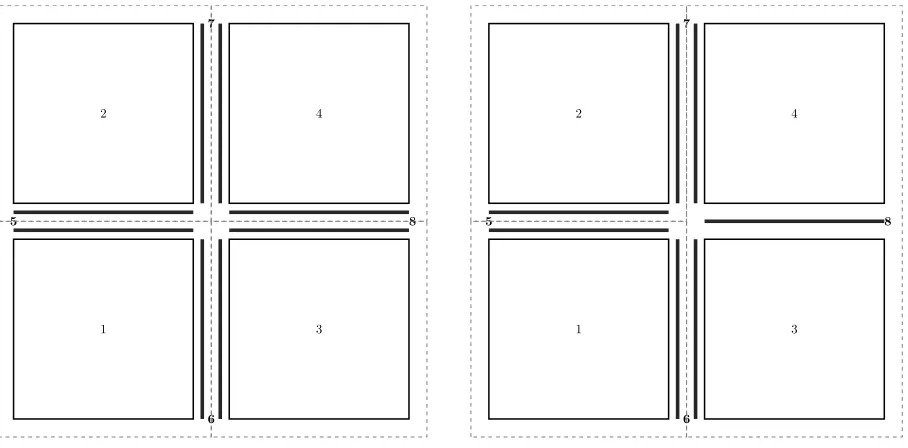
The parallel implementation is designed using the message passing interface(MPI) library. The objective of the parallel implementation is to minimize the amount of communications with respect to the parallel operations involved in the linear solver, namely matrix-vector products and dot products. One of interests of this mortar parallel implementation is that there’s no communication at cross-points(in 2D and 3D) and cross-edges(in 3D), which reduces considerably communications between subdomains.

Assuming a constant number of internal dofs in each subdomain, it is rather straightforward to bind a subdomain to each process. Each process would own its subdomain mesh Thk, functional space Xhk, stiffness matrixAk and unknownuk. Regarding the mortars, the choice is less obvious. In order to decrease the amount of communications in the matrix-vector products, we have used technique developed in [2] which consists in duplicating the data at the interfaces between subdomains. If Γkl is such an interface, then the Lagrange multiplier vectorλkland its associated trace meshThk,l and trace spaceMhk,l are stored in both the processors dealing Ωk and Ωl. Although the data storage is increased a little bit, the communications will be reduced significantly.

1

5

6

2

7

3

8

4

1.1. One subdomain per cluster

1

5

6

2

7

3

8

4

1.2. Subdomains 3 and 4 on the same cluster

Figure 1. Domain decompositions

neighboring subdomains belong to different clusters, there are two copies of the mortar interface variables stored in different clusters. Consider the interfaces as shown in the picture. The matrixAhas the following form:

A=            

A1 BT15 BT16 0 0

A2 BT25 0 B27T 0

A3 0 BT36 0 B38T

A4 0 0 B47T B48T

B15 B25 0 0

B16 0 B36 0

0 B27 0 B38

0 0 B47 B48

           

Let us consider the matrix-vector multiplication procedure with the matrix A and the vector (˜u,˜λ), where ˜u

and ˜λhave the following component-wise representation, according to the decomposition and the enumeration in _Figure 1.1.: ˜u= (uT₁, u₂T, uT₃, uT₄)T and ˜λ= (λ₅T, λT₆, λT₇, λT₈)T. The resulting vector (v˜,µ˜) =A ·(u˜,˜λ) can be computed as

             

v₁(1) v₂(2) v₃(3) v₄(4) µ(1₅,2) µ(1₆,3) µ(2₇,3) µ(3₈,4)

              =              

A1u(1)₁ +B₁₅Tλ(1)₅ +B₁₆Tλ(1)₆ A2u(2)₂ +B₂₅Tλ(2)₅ +B₂₇Tλ(2)₇ A3u(3)₃ +B₃₆Tλ(3)₆ +B₃₈Tλ(3)₈ A4u(4)₄ +B₄₇Tλ(4)₇ +B₄₈Tλ(4)₈ B15u

(1)

1 +B25u (2) 2 B16u

(1)

1 +B36u (3) 3 B27u

(2)

2 +B47u (4) 4 B38u

(3)

3 +B48u (4) 4               (7)

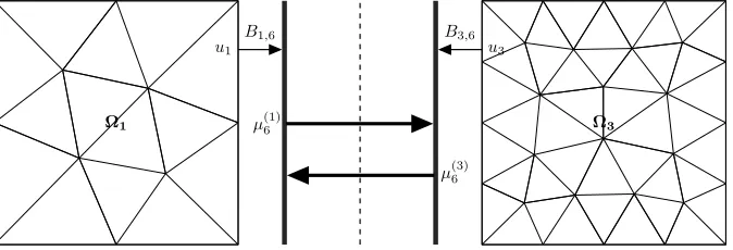
where the upper indices denote the cluster(the processor), in which this variable is stored. Two upper indices mean that this variable is stored in both processors. Note thatλ(_ik)≡λ(_il)and so far we need communications only when computingµi. For example

Ω1

u1

B1,6

µ(1)₆ Ω3

u3

B3,6

µ(3)6

Figure 2. Communications for jump matrix multiplication

µ6=µ(1)₆ +µ(3)₆ , µ(1)₆ =B16u1 and µ(3)₆ =B36u3.

A1 u1

B1,5 B1t,5 λ

(1) 5

B1,6

Bt

1,6

λ(1)₆

µ(1)₅

µ(3)₆

A2 u2

B2,5 B2t,5 λ

(2) 5

Bt

2,7

Bt

2,7

λ(2)₇

µ(2)₅

µ(2)₇

A3 u3

B3,8 B3t,8 λ

(3) 8

B3,6

Bt

3,6

λ(3)₆

µ(1)₆

µ(4)₈

A4 u4

Bt

4,7

B4,7

λ(4)₇

B4,8 B4t,8 λ

(4) 8

µ(4)₇

µ(3)₈

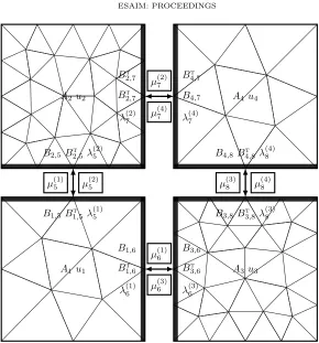
Figure 3. Communications for parallel matrix-vector multiplication

For the _Feel++ [16,17] implementation the communications are handled explicitly by the user and we use _PETSc [3–5,14] sequentially even though the code is parallel using MPI communicators. This technique requires explicitly sending and receiving complex data structures such as mesh data structures,_PETScvectors and elements of functions space(traces) usingBoost.MPIandBoost.Serialization[1].

4.

Numerical Results

We present in this section the numerical results of the parallel implementation of the mortar element method described in the section (3) using _Feel++and Boost.MPIlibraries. We consider here the problem (2) in 3D with g = sin(πx) cos(πy) cos(πz) the exact solution and f =−∆g = 3π2_{g the corresponding right hand side.}

The problem is solved in the parallelepiped Ω = [0, Lx]×[0, Ly]×[0, Lz], Lx, Ly, Lz>0. The following numerical results are obtained usingP2finite element approximations in each subdomain Ωk withhΩk = 0.1 in the strong scaling study(see subsection 4.1) and hΩ_k = 0.075 in the weak scaling one(see subsection4.2), k = 1,· · ·, L. The stopping criterion is such that the residual norm for the Krylov solver is less thanε= 10−7.

The simulations have been performed at Leibniz Supercomputing Centre (LRZ) on SuperMUC. SuperMUC is the Tier-0 supercomputer with 155.656 processor cores in 9400 compute nodes which provides resource to PRACE via the German Gauss Centre. The system is an IBM System x iDataPlex based on Intel Sandy Bride EP processors. SuperMUC has a peak performance of 3.2 PFLOP/s consisting of 18 islands, each combining 512 compute nodes with 16 physical cores and 32 GB per node. The nodes are connected by a non-blocking fat tree, based on Infiniband FDR10.

The first is thestrong scaling, which is defined as how the solution time varies with the number of cores for a fixed total problem size. The goal is to minimize time to solution for a given problem by keeping the problem size fixed and increasing the number of cores.

The second is the weak scaling, which is defined as how the solution time varies with the number of cores for a fixed problem size per core. The goal is to solve the larger problems by keeping the work per core fixed and increasing the number of cores.

4.1.

Strong Scaling

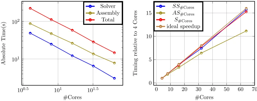
We present here the strong scaling results corresponding to the partition of the global domain Ω intoLx×

Ly×Lzsubdomains (1 subdomain per core) with the fixed lengthsLx=Ly=Lz= 1. We plot inFigure4.1. the absolute solve time and assembly time and total time versus the number of cores in loglog axis and in

Figure4.2. the speedup and ideal speedup versus number of cores. The total number of degrees of freedom is

approximately equal to 500.000 and all the the measured timings are expressed in seconds.

We define the speedup by the following formula: Sp=Tr/Tp where pis the number of cores and Tr the execution time of the parallel algorithm with r cores(r = 4 is our reference number of cores) and Tp the execution time of the parallel algorithm withpcores(r < p). Analogously we define by SSp the corresponding speedup for the solver time and byASp for assembly.

100.5 ₁₀1 ₁₀1.5

101 102

#Cores

Absolute

Time(s)

Solver Assembly

Total

4.1. Absolute Solve and Total time versus #Cores

0 10 20 30 40 50 60 70

0 5 10 15

#Cores

Timing

relativ

e

to

4

C

or

e

s _ASSS#Cores

#Cores S#Cores ideal speedup

4.2. Speedup versus #Cores

Figure 4. Strong scaling

Remarque 4.1. We observe in_Figure4.2. that the speedup related to the total computational time is very over the ideal speedup. This is due to the fact that the functions spaces construction and matrix factorization timings decrease significantly in the strong scaling, as well as the communications between subdomains which are few in only 24 cores. We expect to find the normal behavior on the large scale architectures on which we can take many subdomains with more consistent problem size.

4.2.

Weak Scaling

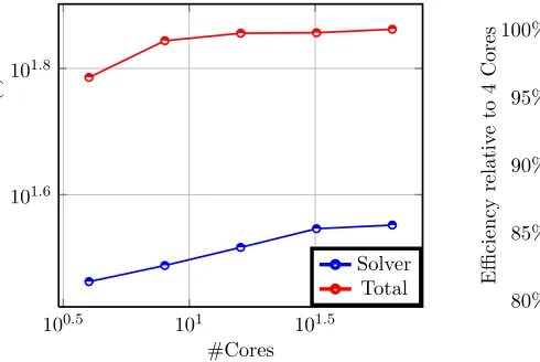
We present here the the weak scaling results corresponding to the partition of the global domain Ω into

Lx×Ly×Lz subdomains (1 subdomain per processor) withLx×Ly×Lz= #Cores. We plot inFigure5.1.

the absolute solve time and total time versus the number of cores in loglog axis and in _Figure 5.2. the

number of degrees of freedom is approximately equal to 30.000 per subdomain and all the measured timing are expressed in seconds.

100.5 ₁₀1 ₁₀1.5

101.6 101.8

#Cores

Absolute

Time(s)

Solver Total

5.1. Absolute Solve and Total time versus #Cores

0 10 20 30 40 50 60 70

80% 85% 90% 95% 100%

#Cores

Efficiency

relativ

e

to

4

Cores

ES#Cores E#Cores

5.2. Efficiency versus #Cores

Figure 5. Weak scaling

Remarque 4.2. The plots inFigure5.1. clearly show that the absolute solve and total time does not increase significantly when the number of cores and the problem size increase by keeping the problem size per core. This confirms the results expected for the weak scaling study.

4.3.

Convergence Results

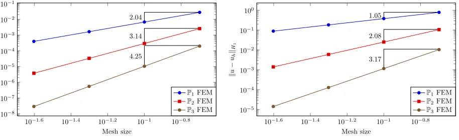
We summarize in the following Tables Table 1. and Table 2. the behavior of L2 and H1 errors of the

numerical solution relative to the analytical solution of our problem using the mortar finite formulation described in the section 2 according to the maximum mesh size h∈ {0.2,0.1,0.05,0.025} and the Lagrange polynomial orders PN, N ∈ {1,2,3}. The tests are performed in the nonconforming case where the characteristic mesh size in the subdomain Ωk ishΩk =h+δk, k= 1,· · · , L, with δk = 0.001 the small perturbation. All the tests are achieved with 2, 4, 8 and 16 number of subdomains. We denote byuthe exact solution of our problem and

uN

h the discrete solution obtained by using the characteristic size equal tohand the piecewise polynomials of degree less than or equal toN. We denotek · k0 theL2-norm andk · k1 theH1-norm. We plot inFigure6.1.

and_Figure6.2. theL2_andH1 _{norms of the error relative to the exact solution versus the characteristic mesh}

sizes inloglogaxis.

Table 1. L2Convergence results

h ku−u1

hk0 ku−u2hk0 ku−u3hk0

0.2 2.80·10−2 2.67·10−3 2.16·10−4 0.1 6.69·10−3 2.83·10−4 9.58·10−6 0.05 1.66·10−3 3.24·100 5.29·10−7 0.025 4.00·10−4 _3.91·10−6 _3.10·10−8

Table 2. H1 Convergence results

h ku−u1

hk1 ku−u2hk1 ku−u3hk1

0.2 7.92·10−1 1.09·10−1 1.10·10−2 0.1 3.72·10−1 2.44·10−2 1.08·10−3 0.05 1.83·10−1 5.88·10−3 1.25·10−4 0.025 8.93·10−2 _1.43·10−3 _1.49·10−5

10−1.6 ₁₀−1.4 ₁₀−1.2 ₁₀−1 ₁₀−0.8

10−8

10−7

10−6

10−5

10−4

10−3

10−2

10−1

2.04

3.14

4.25

Mesh size

k

u

−

uh

kL

2

P1FEM

P2FEM

P3FEM

6.1.L2_convergence

10−1.6 ₁₀−1.4 ₁₀−1.2 ₁₀−1 ₁₀−0.8

10−5

10−4

10−3

10−2

10−1

100

1.05

2.08

3.17

Mesh size

k

u

−

uh

kH1

P1FEM

P2FEM

P3FEM

6.2.H1_convergence

Figure 6. Convergence curves

5.

Conclusions

This paper clearly shows that our parallel computational framework scales on the small scale architectures for solving the linear system arising from the mortar finite element method in 2D and 3D with the arbitrary number of subdomain partitions using the block-diagonal preconditioners. Our current work is focused on the implementation of the substructuring preconditioners [9,10] for the discrete Steklov-Poincar´e operator on interfaces so that the number of iterations is maintained as low as possible that is needed for a good scaling on very large scale architectures.

Acknowledgements

The authors would like to thank Vincent Chabannes for many fruitful discussions. Abdoulaye Samake and Christophe Prud’homme acknowledge the financial support of the project ANR HAMM ANR-2010-COSI-009.

This work was granted access to the HPC resources of TGCC@CEA made available within the Distributed Euro-pean Computing Initiative by the PRACE-2IP, receiving funding from the EuroEuro-pean Community’s Seventh Framework Programme (FP7/2007-2013) under grant agreement RI-283493 and of SuperMuc@LRZ available within the Distributed European Computing Initiative by the PRACE-3IP under grant agreement RI-312763.

References

[1] Boost c++ libraries. http://www.boost.org.

[2] G.S. Abdoulaev, Y. Achdou, Y.A. Kuznetsov, and C. Prud’homme. On a parallel implementation of the mortar element method.RAIRO-M2AN Modelisation Math et Analyse Numerique-Mathem Modell Numerical Analysis, 33(2):245–260, 1999. [3] Satish Balay, Kris Buschelman, Victor Eijkhout, William D. Gropp, Dinesh Kaushik, Matthew G. Knepley, Lois Curfman McInnes, Barry F. Smith, and Hong Zhang. PETSc users manual. Technical Report ANL-95/11 - Revision 2.1.5, Argonne National Laboratory, 2004.

[4] Satish Balay, Kris Buschelman, William D. Gropp, Dinesh Kaushik, Matthew G. Knepley, Lois Curfman McInnes, Barry F. Smith, and Hong Zhang. PETSc Web page, 2001. http://www.mcs.anl.gov/petsc.

[5] Satish Balay, Victor Eijkhout, William D. Gropp, Lois Curfman McInnes, and Barry F. Smith. Efficient management of parallelism in object oriented numerical software libraries. In E. Arge, A. M. Bruaset, and H. P. Langtangen, editors,Modern Software Tools in Scientific Computing, pages 163–202. Birkh¨auser Press, 1997.

[6] F. Ben Belgacem and Y. Maday. The mortar element method for three-dimensional finite elements.R.A.I.R.O. Mod´el. Math. Anal., 31:289–302, 1997.

[7] M. Benzi, G.H. Golub, and J. Liesen. Numerical solution of saddle point problems.Acta numerica, 14(1):1–137, 2005. [8] C. Bernardi, Y. Maday, and A. Patera. A new nonconforming approach to domain decomposition:the mortar element method.

[9] S. Bertoluzza and M. Pennacchio. Preconditioning the mortar method by substructuring: The high order case.Applied Nu-merical Analysis & Computational Mathematics, 1(2):434–454, 2004.

[10] Silvia Bertoluzza and Micol Pennacchio. Analysis of substructuring preconditioners for mortar methods in an abstract frame-work.Applied Mathematics Letters, 20(2):131 – 137, 2007.

[11] Jie Chen, L.C. McInnes, and H. Zhang. Analysis and practical use of flexible BICGSTAB. Technical Report ANL/MCS-P3039-0912, Argonne National Laboratory, 2012.

[12] H.C. Elman, D.J. Silvester, and A.J. Wathen.Finite Elements and Fast Iterative Solvers:with Applications in Incompressible Fluid Dynamics: with Applications in Incompressible Fluid Dynamics. Numerical Mathematics and Scientific Computation. OUP Oxford, 2005.

[13] G.H. Golub and Q. Ye. Inexact preconditioned conjugate gradient method with inner-outer iteration. SIAM Journal on Scientific Computing, 21(4):1305–1320, 1999.

[14] Vicente Hernandez, Jose E. Roman, and Vicente Vidal. SLEPc: A scalable and flexible toolkit for the solution of eigenvalue problems.ACM Transactions on Mathematical Software, 31(3):351–362, 2005.

[15] M.F. Murphy, G.H. Golub, and A.J. Wathen. A note on preconditioning for indefinite linear systems. SIAM Journal on Scientific Computing, 21(6):1969–1972, 2000.

[16] Christophe Prud’homme. A domain specific embedded language in C++ for automatic differentiation, projection, integration and variational formulations. Scientific Programming, 14(2):81-110, 2006.

[17] Christophe Prud’homme. Life: Overview of a unified C++ implementation of the finite and spectral element methods in 1d, 2d and 3d. In Workshop On State-Of-The-Art In Scientific And Parallel Computing, Lecture Notes in Computer Science, page 10. Springer-Verlag, 2007.

[18] Y. Saad. A flexible inner-outer preconditioned GMRES algorithm. SIAM Journal on Scientific Computing, 14(2):461–469, 1993.

[19] Y. Saad.Iterative methods for sparse linear systems. Society for Industrial and Applied Mathematics, 2003.